Nearshore Sandbar Classification of Sabaudia (Italy) with LiDAR Data: The FHyL Approach

 ,
, 

Abstract
1. Introduction
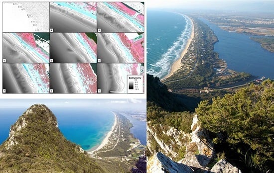
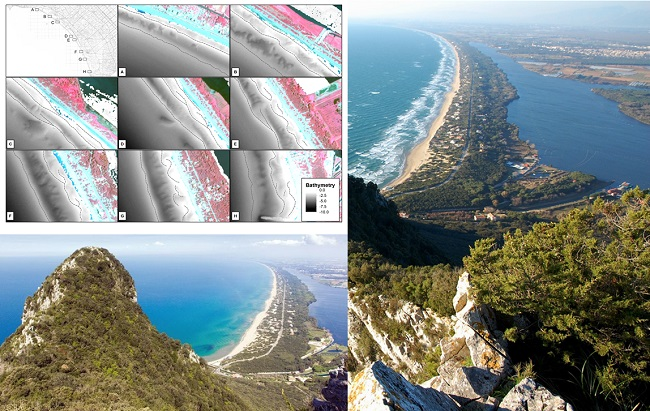
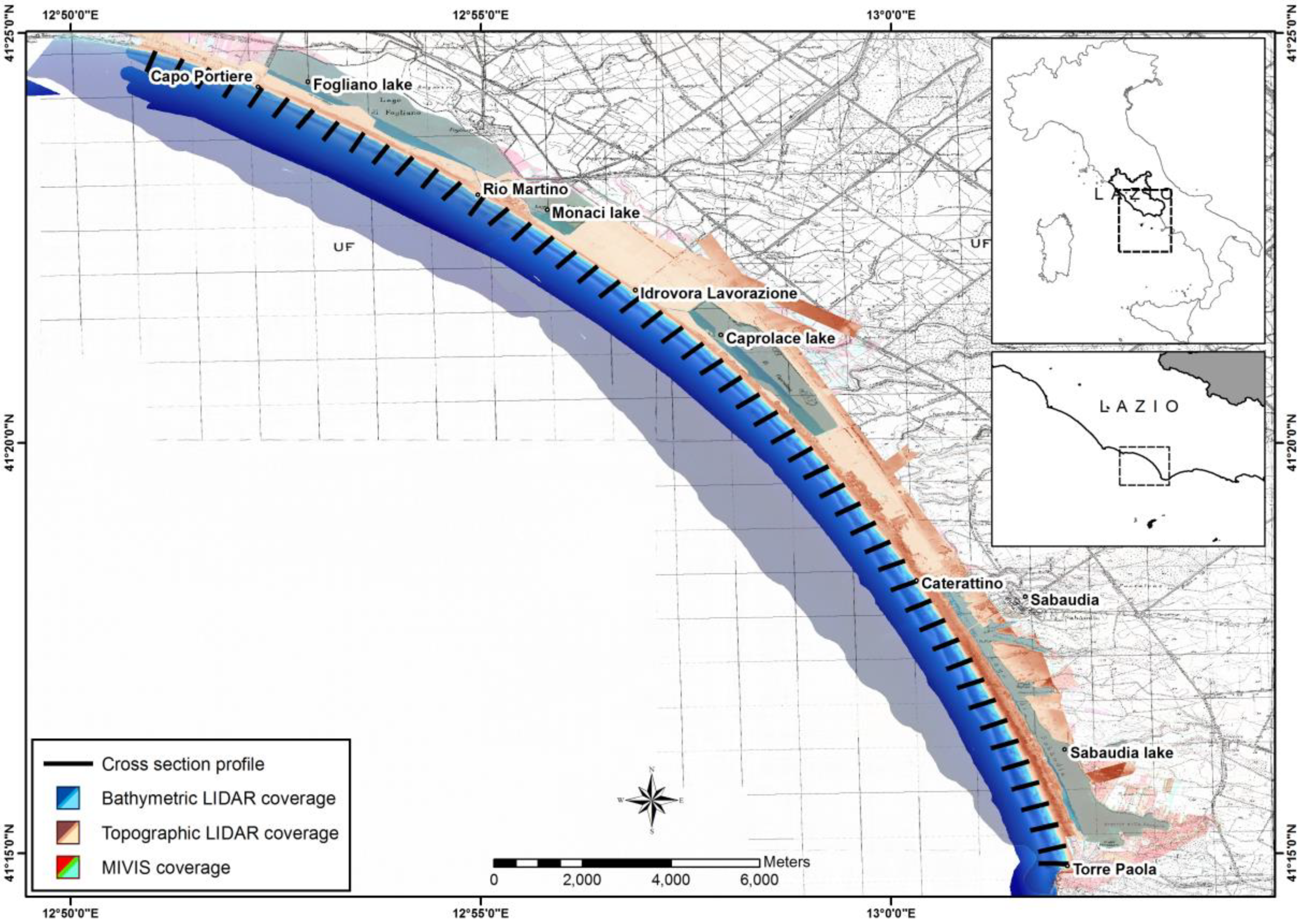
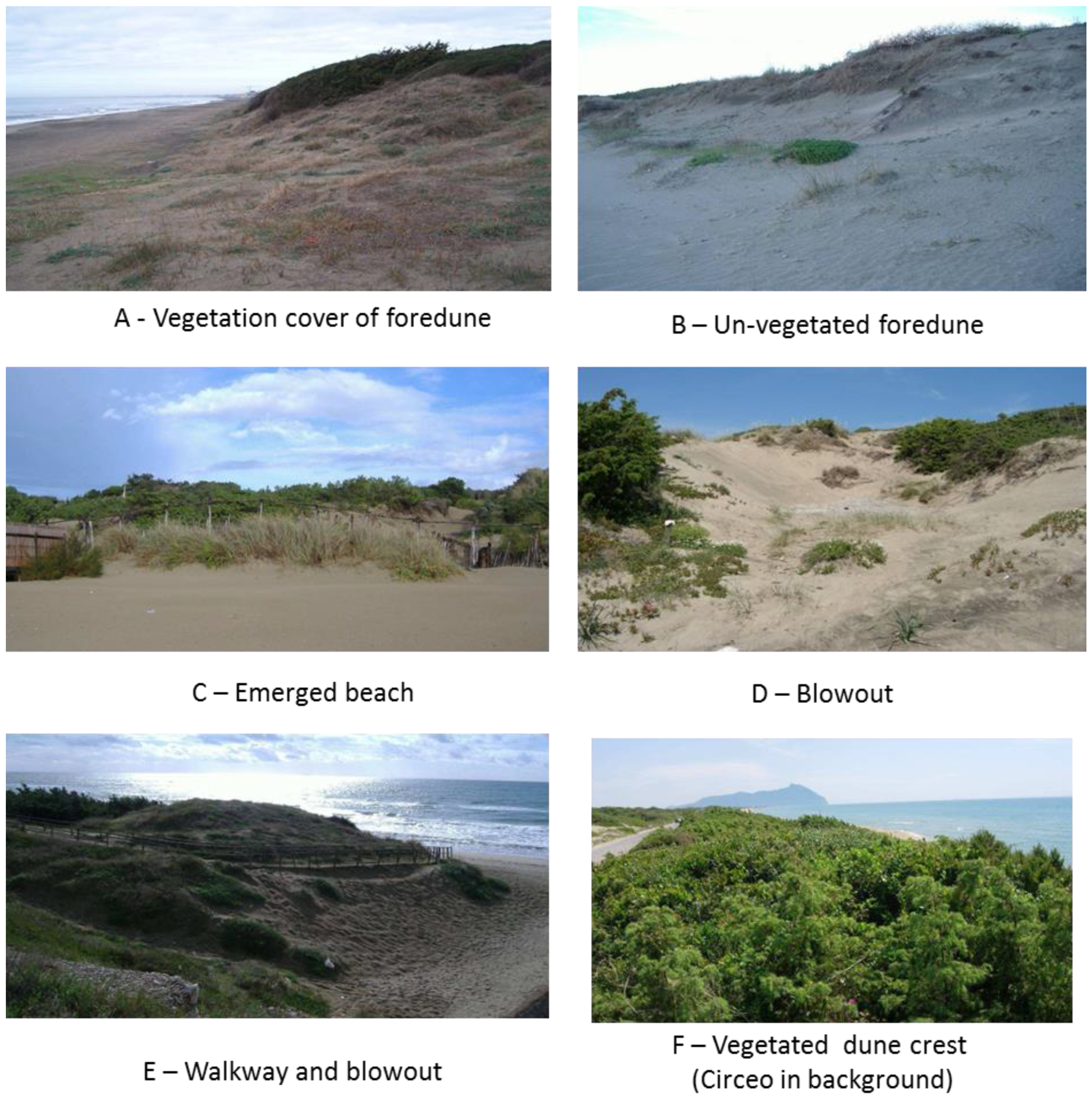
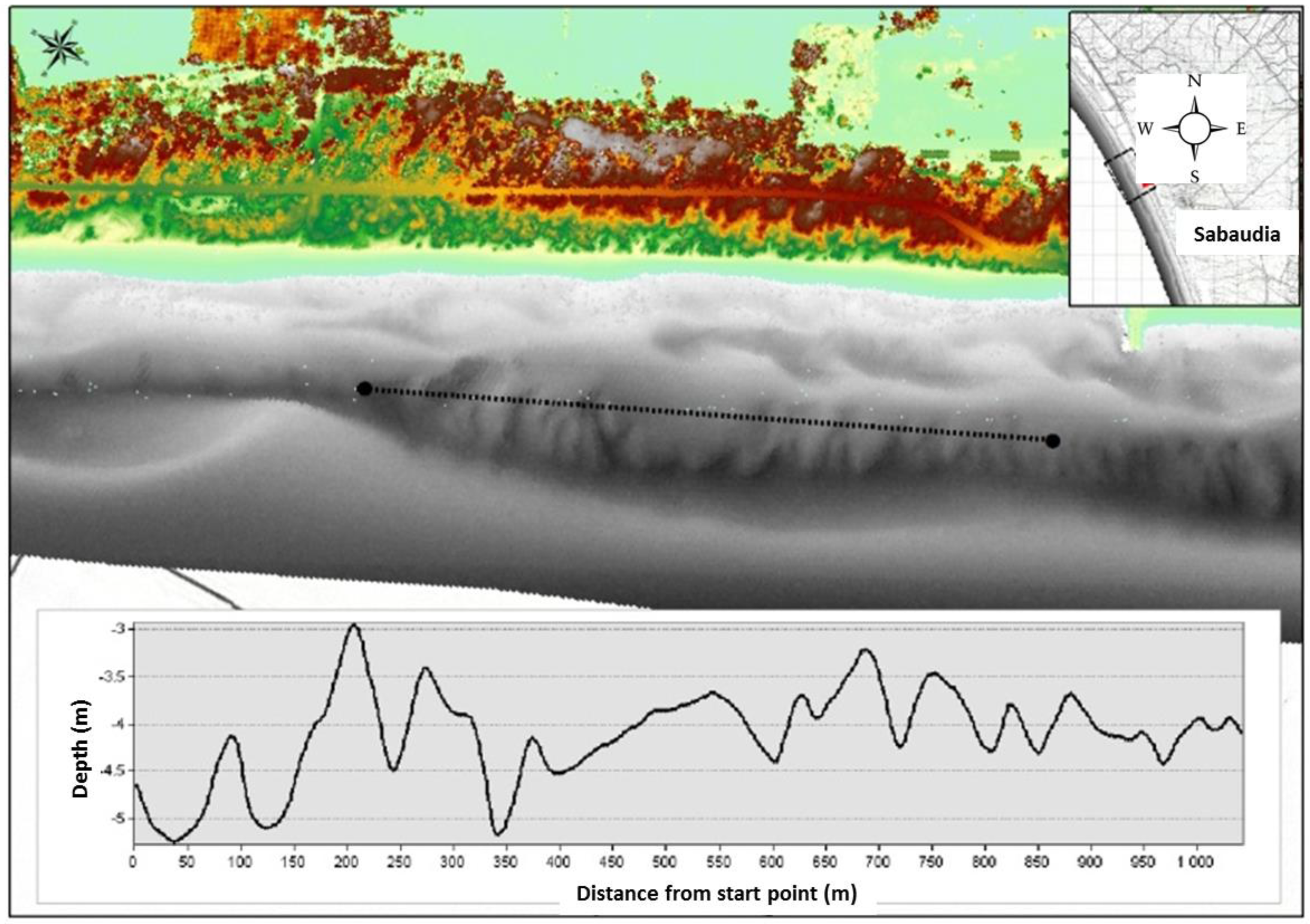
2. Study Area
3. Materials and Methods
3.1. Materials
3.2. Field Measurements
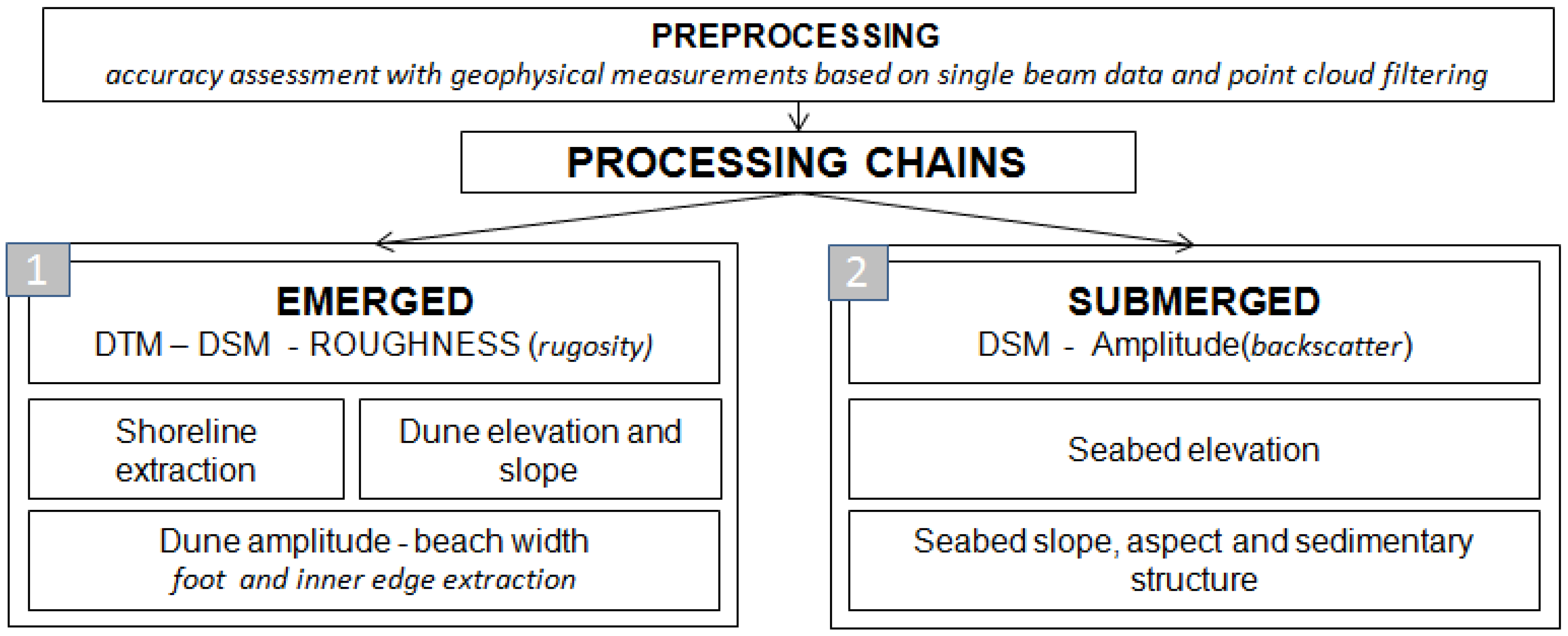
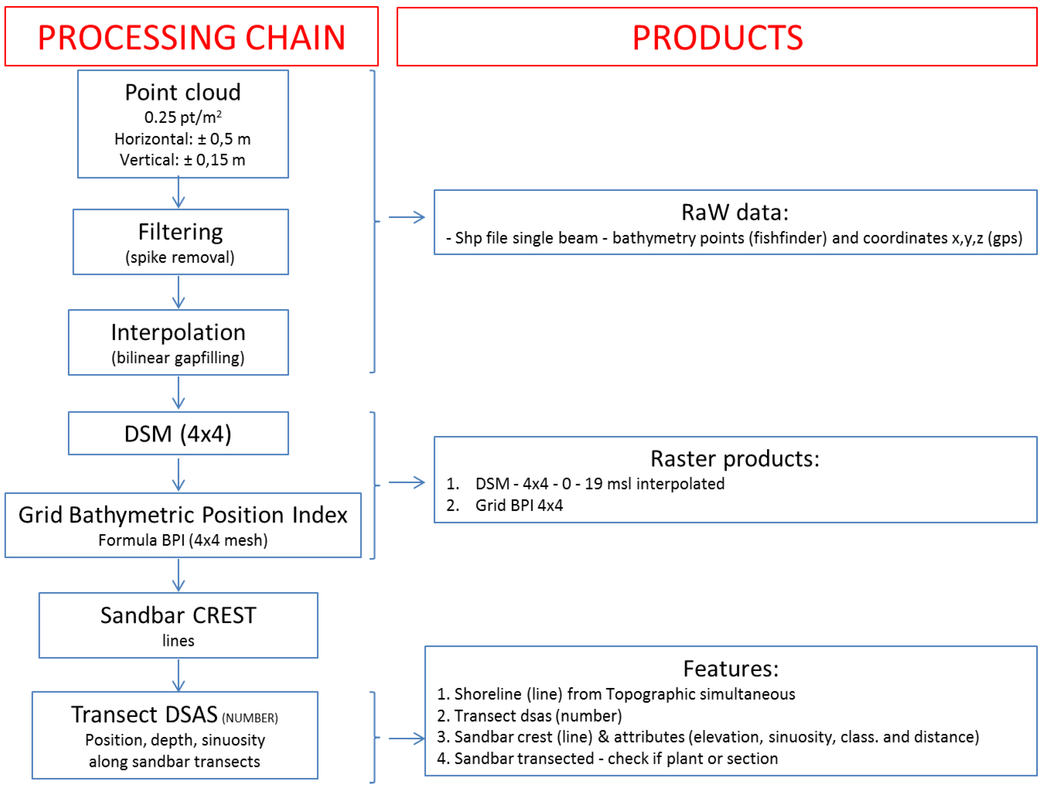
3.3. Methodology
3.3.1. Parameters Extraction from Bathymetric LiDAR Data
3.3.2. DSM Generation: Bathymetry
3.3.3. Bathymetric Position Index (BPI)
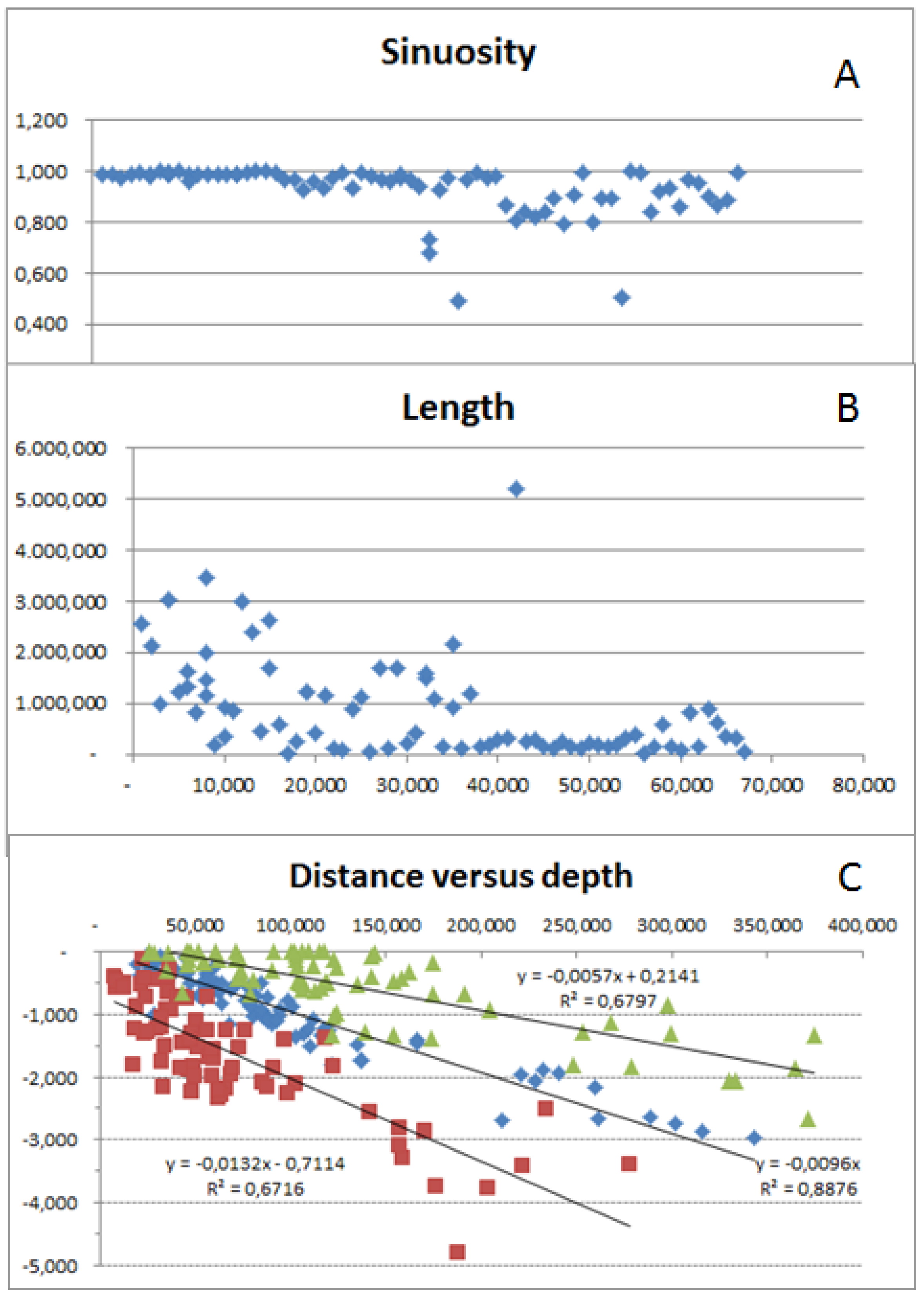
3.3.4. Bars Extraction and Sinuosity
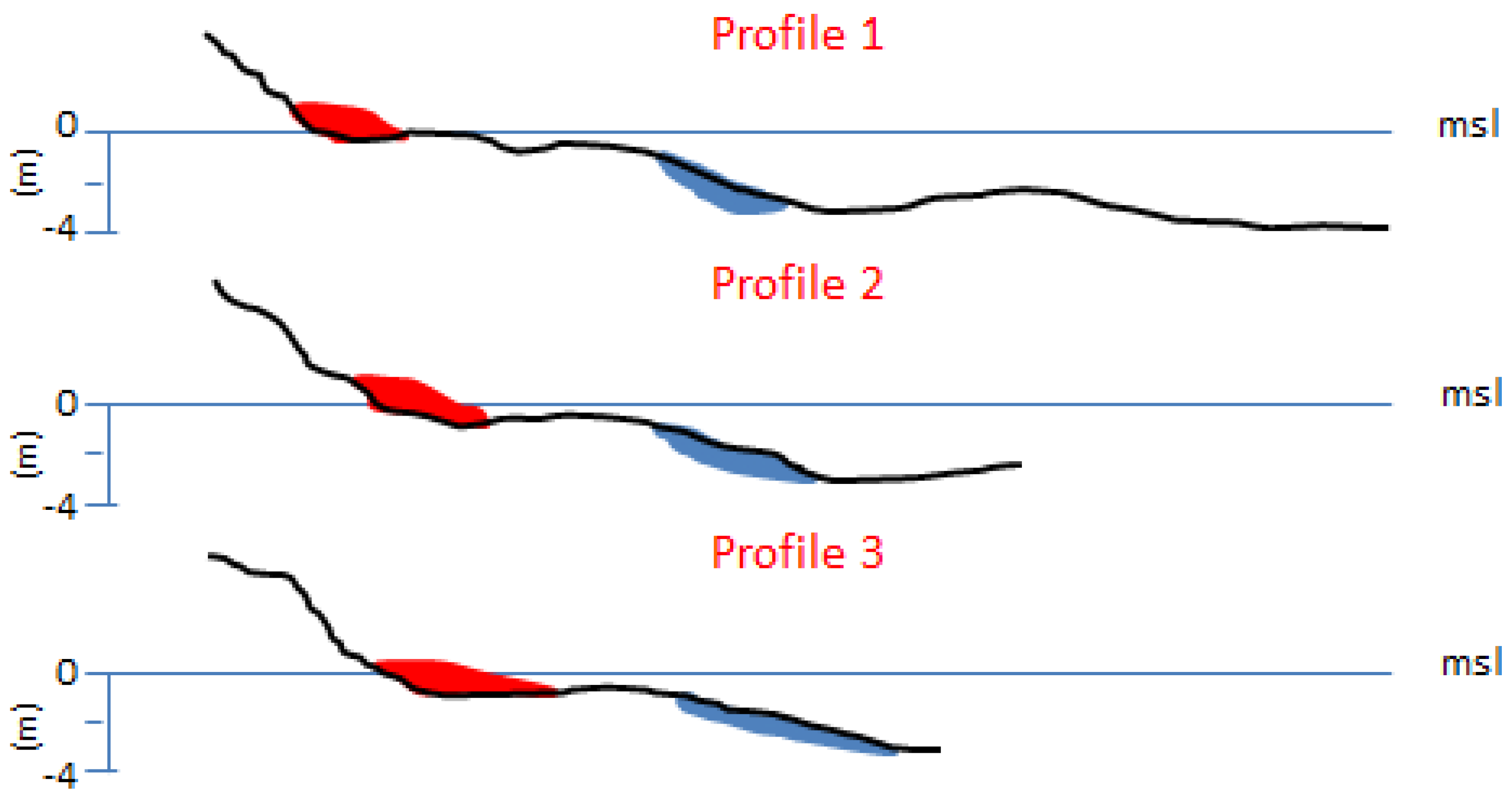
4. Results
- 1.
- Shp file single beam − bathymetry points (fishfinder) and coordinates x,y,z (gps)
- 2.
- DSM – 4 × 4 − 0 − 19 msl interpolated
- 3.
- Grid BPI 4 × 4
- 4.
- Shoreline (from LiDAR)
- 5.
- Transect DSAS
- 6.
- Sandbar crest (line; number 75)
- 7.
- Sandbar parameters (excel file)
- 8.
- Transect parameters (excel file)
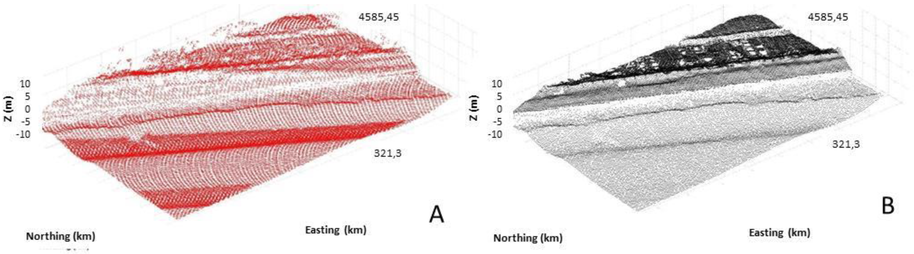
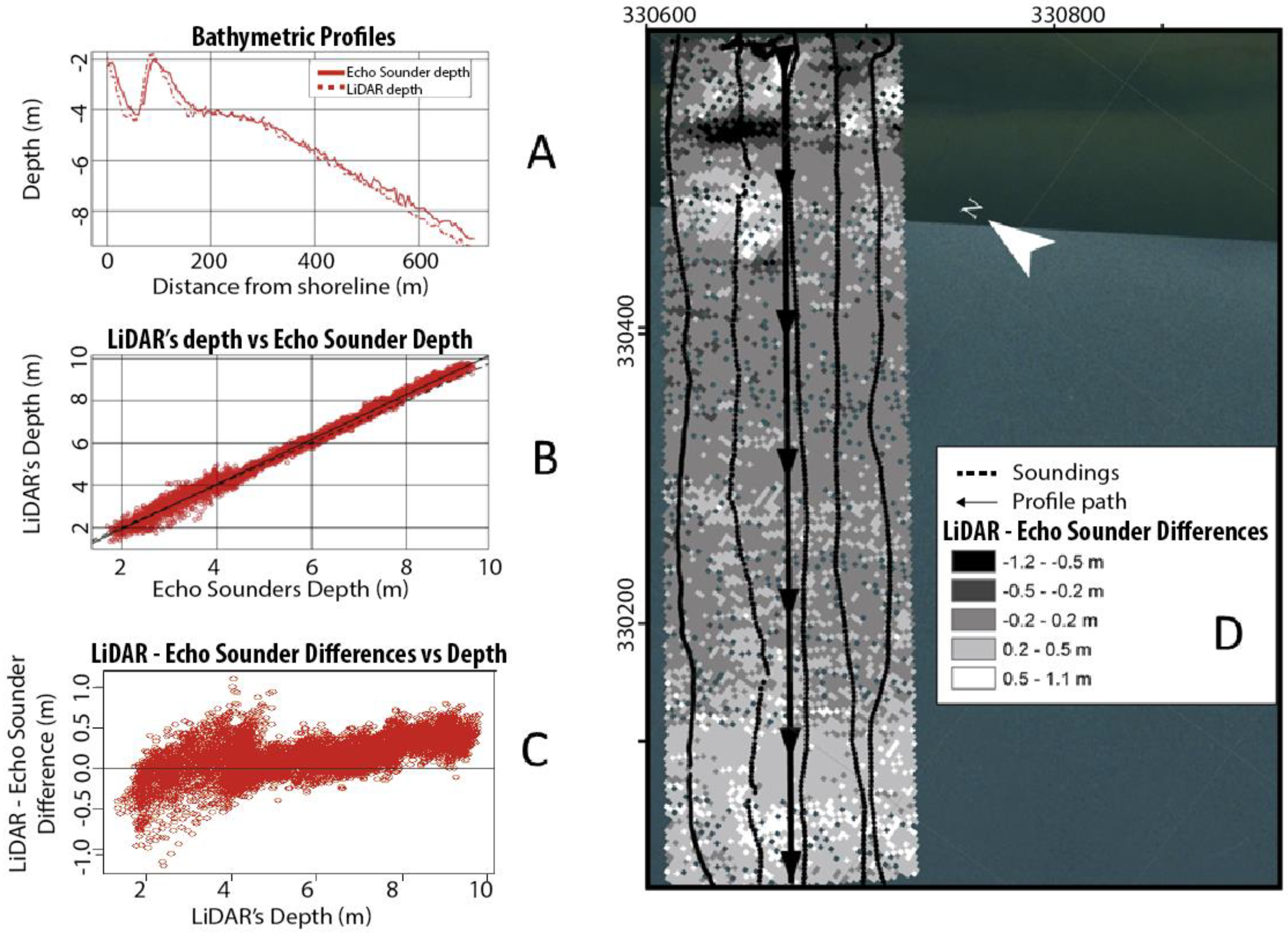
4.1. Results from LiDAR Survey and Accuracy
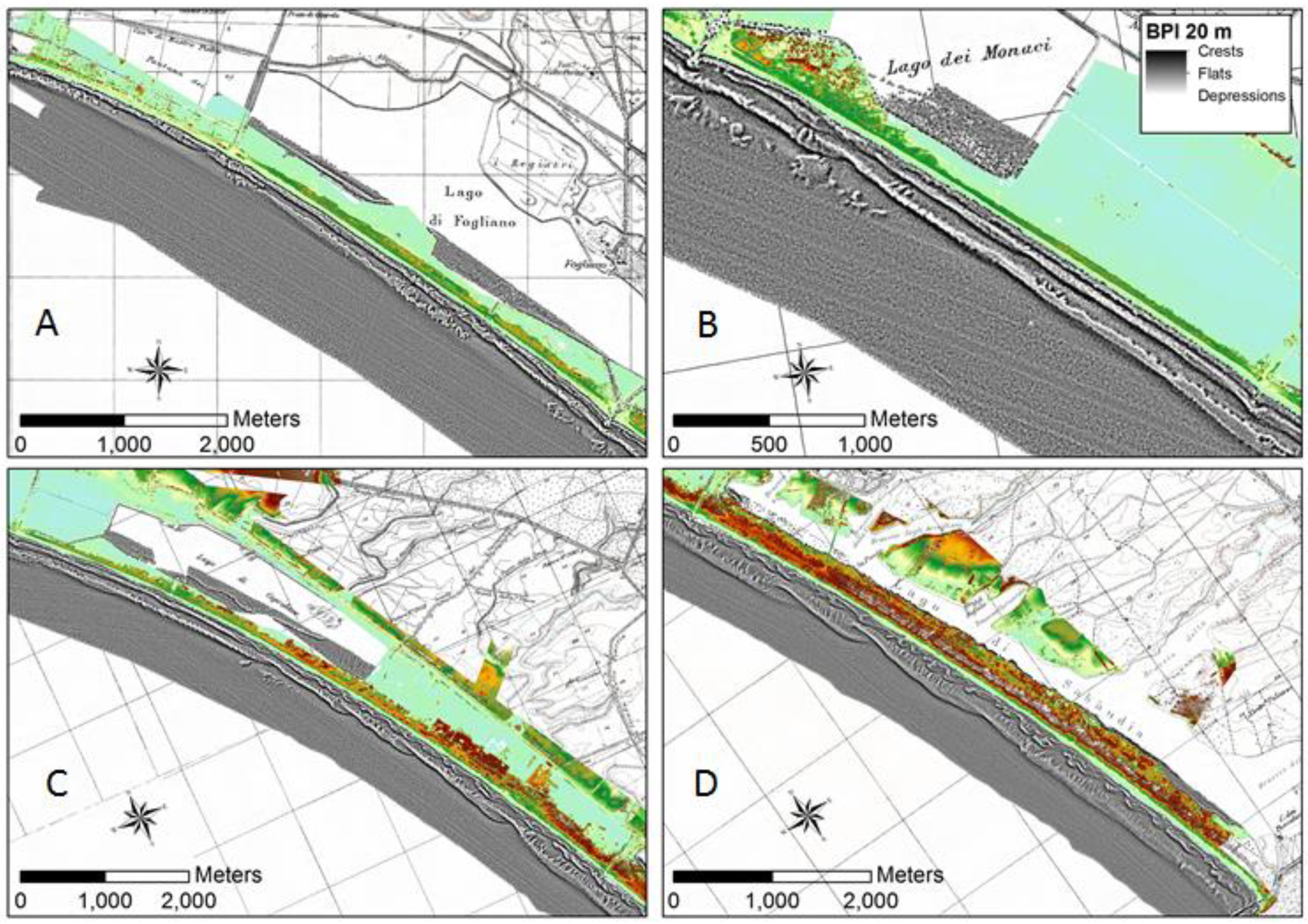
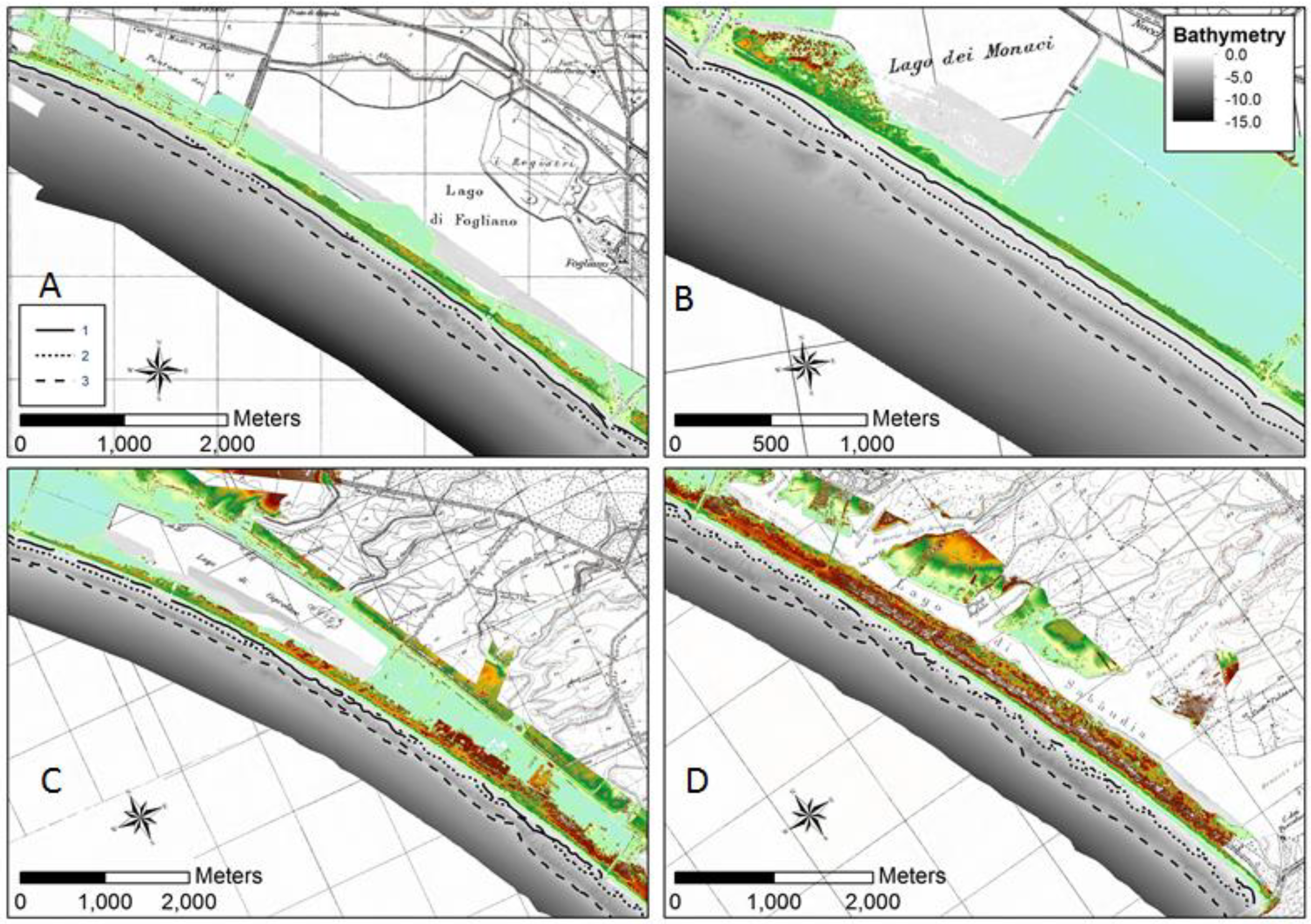
4.2. Bathymetric Position Index (BPI)
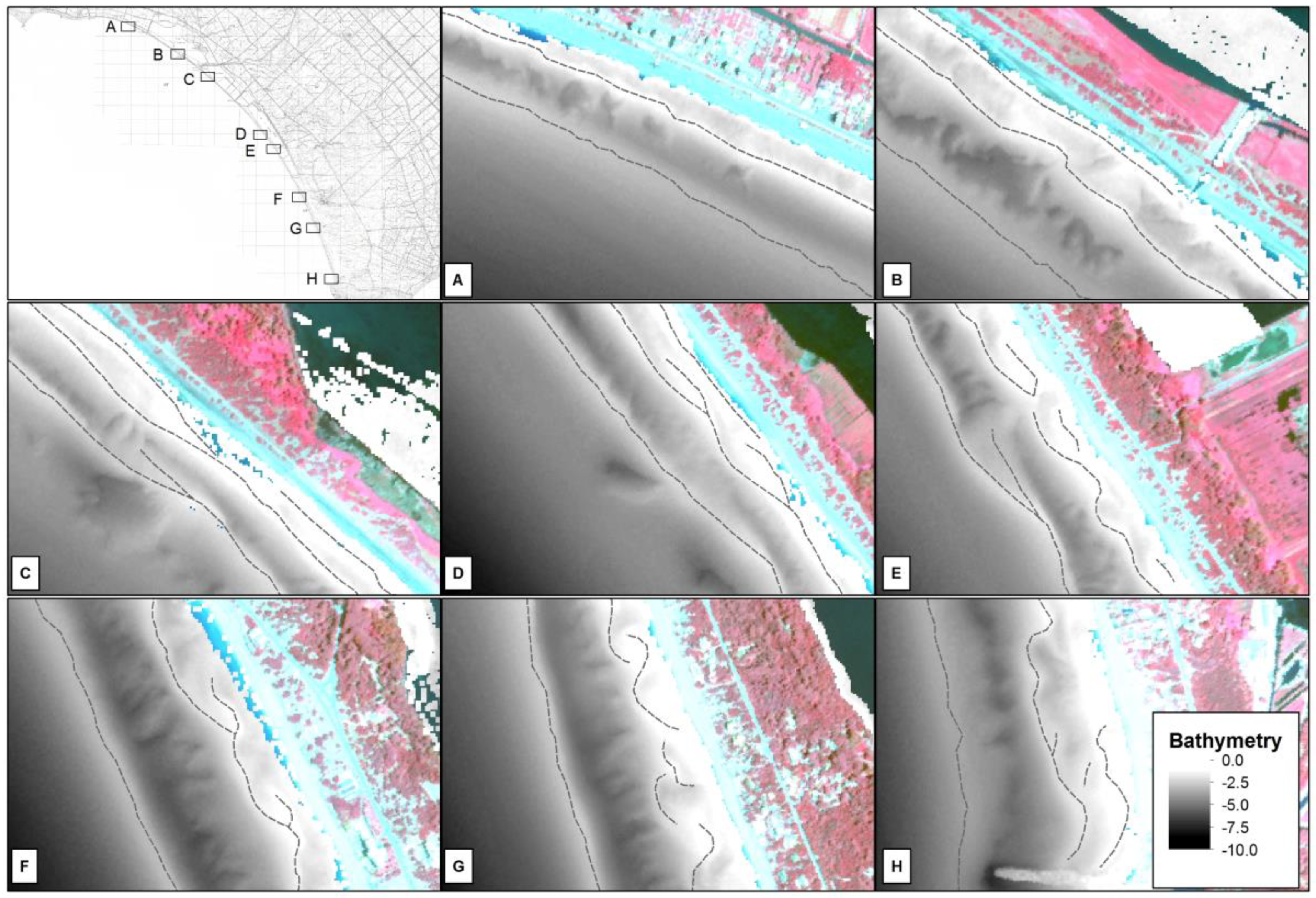
4.3. Submerged Bed FormsObserved in the Nearshore Zone
5. Discussion
5.1. Data Accuracy
5.2. Data Analysis and Elaboration Techniques
5.3. Use of Remote Sensing Products for Coastal Management
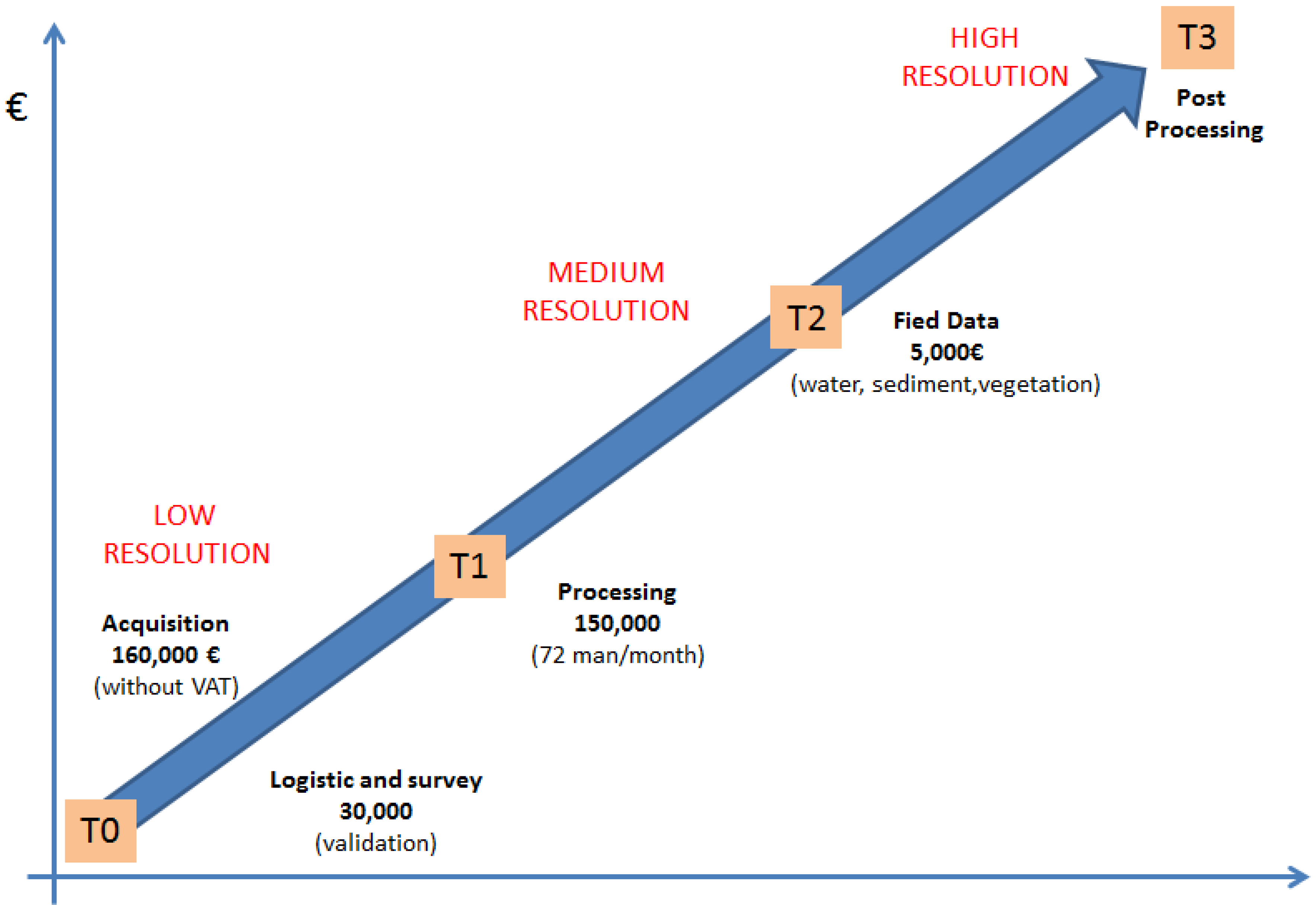
5.4. Cost of Remote Sensing Survey and Contribute of FHyL to National RS Plan
| 1. Airborne multisensory acquisition: | ~ 1600 €/km2 (for about 100 km2) 160,000 € |
| 2. Field data analysis: | ~ 5000 € (see also Valentini et al., 2020, this SI) |
| 3. Logistic and surveys: | ~ 300 €/km2 (fieldwork and dissemination) |
| 4. Processing was 1:1 (man month): | ~ 1500 €/km2 (for about 100 km2) 150,000 € |
| 5. Post processing 1/3: | ~ 530 €/km2 (software, workstation, etc…) |
6. Conclusions
Author Contributions
Funding
Acknowledgments
Conflicts of Interest
References
- Short, A.D. Handbook of Beach and Shoreface Morphodynamics; Wiley: West Sussex, UK, 1999; p. 379. [Google Scholar]
- Armaroli, C.; Grottoli, E.; Harley, M.D.; Ciavola, P. Beach morphodynamics and types of foredune erosion generated by storms along the Emilia-Romagna coastline, Italy. Geomorphology 2013, 199, 22–35. [Google Scholar] [CrossRef]
- Stive, M.J.F.; Aarninkhof, S.G.J.; Hamm, L.; Hanson, H.; Larson, M.; Wijnberg, K.M.; Nicholls, R.J.; Capobianco, M. Variability of shore and shoreline evolution. Coast. Eng. 2002, 47, 211–235. [Google Scholar]
- Benedet, L.; Finkl, C.W.; Campbell, T.; Kleing, A. Predicting the effect of beach nourishment and cross-shore sediment variation on beach morphodynamic assessment. Coast. Eng. 2004, 51, 839–861. [Google Scholar] [CrossRef]
- Kraus, N.C.; Larson, M.; Kriebel, D.L. Evaluation of beach erosion and accretion predictors. Proc. Coast. Sediments Conf. (SeattleAsce) 1991, 1, 572–587. [Google Scholar]
- Van Rijn, L.C. Principles of Coastal Morphology; Aqua Publications: Blokzijl, The Netherlands, 1998; p. 730. [Google Scholar]
- Lipman, T.C.; Holman, R.A. The spatial and temporal variability of sand bar morphology. J. Geophys. Res. 1990, 95, 1575–1590. [Google Scholar] [CrossRef]
- Klein, A.H.F.; Menezes, J.T. Beach morphodynamics and profile sequence for headland bay coast. J. Coast. Res. 2001, 17, 812–835. [Google Scholar]
- Lisi, I.; Molfetta, M.G.; Bruno, M.F.; Di Risio, M.; Damiani, L. Morphodynamic classification of sandy beaches in enclosed basins: The case study of Alimini (Italy). J. Coast. Res. 2011, SI 64, 180–184. [Google Scholar]
- Traganos, D.; Poursanidis, D.; Aggarwal, B.; Chrysoulakis, N.; Reinartz, P. Estimating satellite-derived bathymetry (SDB) with the google earth engine and sentinel-2. Remote Sens. 2018, 10, 859. [Google Scholar] [CrossRef]
- Misra, A.; Vojinovic, Z.; Ramakrishnan, B.; Luijendijk, A.; Ranasinghe, R. Shallow water bathymetry mapping using Support Vector Machine (SVM) technique and multispectral imagery. Int. J. Remote Sens. 2018, 39, 4431–4450. [Google Scholar] [CrossRef]
- Kasvi, E.; Salmela, J.; Lotsari, E.; Kumpula, T.; Lane, S.N. Comparison of remote sensing based approaches for mapping bathymetry of shallow, clear water rivers. Geomorphology 2019, 333, 180–197. [Google Scholar] [CrossRef]
- Agrafiotis, P.; Karantzalos, K.; Georgopoulos, A.; Skarlatos, D. Correcting image refraction: Towards accurate aerial image-based bathymetry mapping in shallow waters. Remote Sens. 2020, 12, 322. [Google Scholar] [CrossRef]
- Dietrich, J.T. Bathymetric structure from motion: Extracting shallow stream bathymetry from multi view stereo photogrammetry. Earth Surf. Process. Landf. 2017, 42, 355–364. [Google Scholar] [CrossRef]
- Guenther, G.C. Airborne Lidar bathymetry. In Digital Elevation Model Technologies and Applications: The DEM Users Manual; American Society of Photogrammetry and Remote Sensing: Bethesda, MD, USA, 2007; pp. 253–320. [Google Scholar]
- Deronde, B.; Houthuys, R.; Debruyn, W.; Fransaer, D.; Lancker, V.V.; Henriet, J.-P. Use of airborne hyperspectral data and laserscan data to study beach morphodynamics along the Belgian coast. J. Coast. Res. 2006, 225, 1108–1117. [Google Scholar] [CrossRef]
- Schwarz, R.; Mandlburger, G.; Pfennigbauer, M.; Pfeifer, N. Design and evaluation of a full-wave surface and bottom-detection algorithm for LiDAR bathymetry of very shallow waters. ISPRS J. Photogramm. Remote Sens. 2019, 150, 1–10. [Google Scholar] [CrossRef]
- Kogut, T.; Bakuła, K. Improvement of full waveform airborne laser bathymetry data processing based on waves of neighborhood points. Geosciences 2019, 11, 1255. [Google Scholar] [CrossRef]
- Manzo, C.; Valentini, E.; Taramelli, A.; Filipponi, F.; Disperati, L. Spectral characterization of coastal sediments using field spectral libraries, airborne hyperspectral images and topographic LiDAR data (FHyL). Int. J. Appl. Earth Obs. Geoinf. 2015, 36, 54–68. [Google Scholar] [CrossRef]
- Adam, S.; De Backer, A.; De Wever, A.; Sabbe, K.; Tooman, E.A.; Vinex, M.; Monbaliu, J. Bio-physical characterization of sediment stability in mudflat using remote sensing: A laboratory experiment. Cont. Shelf Res. 2011, 31 (Suppl. S10), S26–S35. [Google Scholar] [CrossRef]
- Athearn, N.D.; Takekawa, J.Y.; Jaffe, B.; Hattenbach, B.J.; Foxgrover, A.C. Mapping elevations of tidal wetland restoration sites in San Francisco Bay: Comparing accuracy of aerial LiDAR with a singlebeam echosounder. J. Coast. Res. 2010, 26, 312–319. [Google Scholar] [CrossRef]
- Brock, J.C.; Purkis, M.J. The emerging role of LiDAR remote sensing in coastal research and resource management. J. Coast. Res. 2009, 53, 1–5. [Google Scholar] [CrossRef]
- Davidson-Arnott, R.G.D. Conceptual model of the effects of sea level rise on sandy coasts. J. Coast. Res. 2005, 26, 1166–1172. [Google Scholar] [CrossRef]
- Goodman, J.A.; Lee, Z.P.; Ustin, S.L. Influence of atmospheric and sea-surface corrections on retrieval of bottom depth and reflectance using a semi-analytical model: A case study in Kaneohe Bay, Hawaii. Appl. Opt. 2008, 47, F1–F11. [Google Scholar] [CrossRef] [PubMed]
- Malthus, T.J.; Mumby, P.J. Remote sensing of the coastal zone: An overview and priorities for future research. Int. J. Remote Sens. 2003, 24, 2805–2815. [Google Scholar] [CrossRef]
- Taramelli, A.; Valentini, E.; Cornacchia, L.; Bozzeda, F. A hybrid power law approach for spatial and temporal pattern analysis of salt marsh evolution. J. Coast. Res. 2017, 77 (Suppl. S1), 62–72. [Google Scholar] [CrossRef]
- Töyrä, J.; Pietroniro, A. Towards operational monitoring of a northern wetland using geomatics-based techniques. Remote Sens. Environ. 2005, 97, 174–191. [Google Scholar] [CrossRef]
- Prasad, A.D.; Jain, K.; Gairola, A. Mapping of lineaments and knowledge base preparation using geomatics techniques for part of the Godavari and Tapi basins, India: A case study. Int. J. Comput. Appl. 2013, 70, 39–47. [Google Scholar]
- Ajmar, A.; Boccardo, P.; Disabato, F. Rapid Mapping: Geomatics role and research opportunities. Rend. Fis. Acc. Lincei. 2015, 26, 63–73. [Google Scholar] [CrossRef]
- Valentini, E.; Taramelli, A.; Filipponi, F.; Giulio, S. An effective procedure for EUNIS and Natura 2000 habitat type mapping in estuarine ecosystems integrating ecological knowledge and remote sensing analysis. Ocean Coast. Manag. 2015, 108, 52–64. [Google Scholar] [CrossRef]
- Cappucci, S.; Valentini, E.; Monte, M.D.; Paci, M.; Filipponi, F.; Taramelli, A. Detection of natural and anthropic features on small islands. J. Coast. Res. 2017, 77 (Suppl. S1), 73–87. [Google Scholar] [CrossRef]
- Bellucci, G.; Altieri, F.; Bibring, J.P.; Bonello, G.; Langevin, Y.; Gondet, B.; Poulet, F. OMEGA/Mars Express: Visual channel performances and data reduction techniques. Planet. Space Sci. 2006, 54, 675–684. [Google Scholar] [CrossRef]
- Barducci, A.; Guzzi, D.; Marcoionni, P.; Pippi, I. Aerospace wetland monitoring by hyperspectral imaging sensors: A case study in the coastal zone of San Rossore Natural Park. J. Environ. Manag. 2009, 90, 2278–2286. [Google Scholar] [CrossRef]
- Boschetti, M.; Boschetti, L.; Oliveri, S.; Casati, L.; Canova, I. Tree species mapping with Airborne hyper-spectral MIVIS data: The Ticino Park study case. Int. J. Remote Sens. 2007, 28, 1251–1261. [Google Scholar] [CrossRef]
- Calvo, S.; Ciraolo, G.; La Loggia, G. Monitoring Posidonia oceanica meadows in a Mediterranean coastal lagoon (Stagnone, Italy) by means of neural network and ISODATA classification methods. Int. J. Remote Sens. 2003, 24, 2703–2716. [Google Scholar] [CrossRef]
- Giardino, C.; Brando, V.E.; Dekker, A.G.; Strömbeck, N.; Candiani, G. Assessment of water quality in Lake Garda (Italy) using Hyperion. Remote Sens. Environ. 2007, 109, 183–195. [Google Scholar] [CrossRef]
- Marani, M.; Belluco, E.; Ferrari, S.; Silvestri, S.; D’Alpaos, A.; Lanzoni, S.; Feola, A.; Rinaldo, A. Analysis, synthesis and modelling of high-resolution observations of salt-marsh ecogeomorphological patterns in the Venice lagoon. Estuar. Coast. Shelf Sci. 2006, 69, 414–426. [Google Scholar] [CrossRef]
- Marani, M.; Silvestri, S.; Belluco, E.; Ursino, N.; Comerlati, A.; Tosatto, O.; Putti, M. Spatial organization and ecohydrological interactions in oxygen-limited vegetation ecosystems. Water Resour. Res. 2006, 42, W06D06. [Google Scholar] [CrossRef]
- Lazio Region. Monitoring Centre of Integrated Coastal Zone Management. 2020. Available online: http://www.cmgizc.info/index.php?option=com_content&view=category&id=24&Itemid=184&lang=it (accessed on 1 January 2020).
- Pallottini, E.; Cappucci, S.; Taramelli, A.; Innocenti, C.; Screpanti, A. Variazioni morfologiche stagionali del sistema spiaggia-duna del Parco Nazionale del Circeo. Studi Costieri 2010, 17, 105–124. [Google Scholar]
- Campo, V.; La Monica, G.B. Le dune costiere oloceniche prossimali lungo il litorale del Lazio. Studi Costieri 2006, 11, 31–42. [Google Scholar]
- Blanc, A.C.; Segre, A. Le auaternaire du monte circeo. Livret guide. In Proceedings of the IV Congrès INQUA, Rome, Italy; 1953, pp. 23–108. Available online: https://www.google.com.hk/url?sa=t&rct=j&q=&esrc=s&source=web&cd=3&ved=2ahUKEwilnryV4bfoAhVU7WEKHWjCCAIQFjACegQIBhAB&url=https%3A%2F%2Fbooks.google.com%2Fbooks%2Fabout%2FINQUA.html%3Fid%3Dnv7nM2CWO4sC&usg=AOvVaw1H7uWKDdmQmv9rr3Ofxv6K (accessed on 14 February 2020).
- Giovagnotti, C.; Rondelli, F.; Pascoletti, F.T. Caratteristiche geomorfologiche e sedimentologiche delle formazioni quaternarie del litorale laziale tra T.re Astura e il M. Circeo. Estratto Degli Annu. Della Fac. Agrar. Dell’università Perugia 1980, 34, 173–235. [Google Scholar]
- Pallottini, E.; Cappucci, S. Beach—Dune system interaction and evolution. Rend. Online Soc. Geol. Ital. 2009, 8, 87–97. [Google Scholar]
- Koppari, K.; Karlsson, U.; Steinvall, O. Airborne laser depth sounding in Sweden. International hydrographic review. Monaco 1994, 71, 69–90. [Google Scholar]
- Schnurr, D. High speed Hawk Eye delivers new efficiencies in coastal zone mapping. Port Eng. Manag. 2009, 27, 2. [Google Scholar]
- Guenther, G.C.; LaRocque, P.E.; Lillycrop, W.J. Multiple surface channels in Scanning Hydrographic Operational Airborne LiDAR Survey (SHOALS) airborne LiDAR. In Proceedings of the Ocean Optics XII, Bergen, Norway, 13–15 June 1994; pp. 422–430. [Google Scholar]
- Thomas, R.W.L.; Guenther, G.C. Water surface detection strategy for an airborne laser bathymeter. In Proceedings of the Ocean Optics X, Orlando, FL, USA, 1 September 1990; p. 597. [Google Scholar]
- Guenther, G.C. Wind and nadir angle effects on airborne LiDAR water’surface’ returns. In Proceedings of the Ocean optics VIII, Orlando, FL, USA, 31 March–2 April 1986; pp. 277–286. [Google Scholar]
- Guenther, G.C.; Thomas, R.W.L. Prediction and Correction of Propagation-induced Depth Measurement Biases Plus Signal Attenuation and Beam Spreading for Airborne Laser Hydrography; NOAA Technical Report NOS: Rockville, MD, USA, 1984. Available online: http://www.ngs.noaa.gov/PUBS_LIB/PredictionAndCorrectionOfPropagationInducedDepthMeasurementBiasesForAirborneLaserHydrography_TR_NOS106_CGS2.pdf (accessed on 19 March 2020).
- ISPRA. Rilievo di Dettaglio Della Batimetria Costiera Laziale con Tecnologie Lidar e Valutazione Delle Caratteristiche Fisiche e Biologiche in Aree Marine Della Costa Laziale di Specifico Interesse Ambientale Fase 2-Caratterizzazione Morfologica; ISPRA: Rome, Italy, 2009; 120p.
- Available online: http://www.caris.com/products/hips-sips/ (accessed on 14 February 2020).
- Available online: http://woodshole.er.usgs.gov/project-pages/dsas/ (accessed on 14 February 2020).
- Available online: http://www.cmgizc.info/index.php?option=com_content&view=article&id=33:lidar-convenzione-ispra&catid=24&Itemid=184&lang=it (accessed on 14 February 2020).
- Taramelli, A.; Valentini, E.; Innocenti, C.; Cappucci, S. FHyL: Field spectral libraries, airborne hyperspectral images and topographic and bathymetric LiDAR data for complex coastal mapping. In Proceedings of the 2013 IEEE International Geoscience and Remote Sensing Symposium-IGARSS, Melbourne, Australia, 21–26 July 2013; pp. 2270–2273. [Google Scholar]
- Irish, J.L.; White, T.E. Coastal engineering applications of high-resolution LiDAR bathymetry. Coast. Eng. 1998, 35, 47–71. [Google Scholar] [CrossRef]
- Quadros, N.D.; Collier, P.A.; Fraser, C.S. Integration of bathymetric and topographic LiDAR: A preliminary investigation. Int. Arch. Photogramm. Remote Sens. Spat. Inf. Sci. 2008, 37, 1299–1304. [Google Scholar]
- Shepard, F.P. Beach cycles in southern California. In Technical Memorandum; Beach Erosion Board, US Army Corps of Engineers: Washington, DC, USA, 1950; Volume 20, p. 31. [Google Scholar]
- Verfaillie, E.; Van Lancker, V.; Van Meirvenne, M. Multivariate geostatistics for the predictive modelling of the surficial sand distribution in shelf seas. Cont. Shelf Res. 2006, 26, 2454–2468. [Google Scholar] [CrossRef]
- Lucieer, V.L. Spatial Uncertainty Estimation Techniques for Shallow Coastal Seabed Mapping; University of Tasmania: Hobart, Australia, 2007; Available online: http://eprints.utas.edu.au/1919/ (accessed on 19 March 2020).
- Micallef, A.; Le Bas, T.P.; Huvenne, V.A.I.; Blondel, P.; Huhnerbach, V.; Deidun, A. A multi-method approach for benthic habitat mapping of shallow coastal areas with high-resolution multibeam data. Cont. Shelf Res. 2012, 39–40, 14–26. [Google Scholar] [CrossRef]
- Diesing, M.; Thorsnes, T. Mapping of cold-water coral carbonate mounds based on geomorphometric features: An object-based approach. Geosciences 2018, 8, 34. [Google Scholar] [CrossRef]
- Janowski, L.; Trzcinska, K.; Tegowski, J.; Kruss, A.; Rucinska-Zjadacz, M.; Pocwiardowski, P. Nearshore benthic habitat mapping based on multi-frequency, multibeam echosounder data using a combined object-based approach: A case study from the Rowy site in the southern Baltic sea. Remote Sens. 2018, 10, 1983. [Google Scholar] [CrossRef]
- Fogarin, S.; Madricardo, F.; Zaggia, L.; Sigovini, M.; Montereale-Gavazzi, G.; Kruss, A.; Lorenzetti, G.; Manfé, G.; Petrizzo, A.; Molinaroli, E.; et al. Tidal inlets in the Anthropocene: Geomorphology and benthic habitats of the Chioggia inlet, Venice Lagoon (Italy). Earth Surf. Process. Landf. 2019, 44, 2297–2315. [Google Scholar] [CrossRef]
- Toso, C.; Madricardo, F.; Molinaroli, E.; Fogarin, S.; Kruss, A.; Petrizzo, A.; Pizzeghello, N.M.; Sinapi, L.; Trincardi, F. Tidal inlet seafloor changes induced by recently built hard structures. PLoS ONE 2009, 14, 29. [Google Scholar] [CrossRef]
- Misiuk, B.; Diesing, M.; Aitken, A.; Brown, C.J.; Edinger, E.N.; Bell, T. A Spatially Explicit Comparison of quantitative and categorical modelling approaches for mapping seabed sediments using random forest. Geosciences 2019, 9, 254. [Google Scholar] [CrossRef]
- Wilson, M.F.J.; O’Connell, B.C.; Brown, J.C.; Guinan, E.; Grehan, A.J. Multiscale terrain analysis of multibeam bathymetry data for habitat mapping on the continental slope. Mar. Geod. 2007, 30, 3–35. [Google Scholar] [CrossRef]
- Sorichetta, A.; Seeber, L.; Taramelli, A.; McHugh, C.; Cormier, M. Geomorphic evidence for tilting at a continental transform: The Karamursel Basin along the North Anatolian Fault, Turkey. Geomorphology 2010, 119, 221–231. [Google Scholar] [CrossRef]
- Taramelli, A.; Valentini, E.; Cornacchia, L.; Monbaliu, J.; Sabbe, K. Indications of dynamic effects on scaling relationships between channel sinuosity and vegetation patch size across a salt marsh platform. J. Geophys. Res. Earth Surf. 2018, 123, 2714–2731. [Google Scholar] [CrossRef]
- Conti, M.; Cappucci, S.; La Monica, G.B. Sediment dynamic of nourished sandy beaches. Rend. Line Soc. Geol. Ital. 2009, 8, 31–38. [Google Scholar]
- Ausili, A.; Cappucci, S.; Gabellini, M.; Innocenti, C.; Maffucci, M.; Romano, E.; Rossi, L.; Taramelli, A. New approaches for multi source data sediment characterisation, thickness assessment and clean up strategies. Chem. Eng. Trans. 2012, 28, 223–228. [Google Scholar]
- Komar, P.D. Beach Processes and Sedimentation; Prentice-Hall: Englewood Cliff, NJ, USA, 1998; p. 429. [Google Scholar]
- Isaksson, A. Coastal Survey Studio Mark II Manual Version 2.X; Airborne Hydrography AB: Jönköping, Sweden, 2009. [Google Scholar]
- Schnurr, D. How low can you go? Maximum depth achieved with Hawk Eye II during project in 2009. In Proceedings of the International LiDAR mapping forum, Denver, CO, USA, 3–5 March 2010. [Google Scholar]
- Finkl, C.W.; Makowski, C. Autoclassification versus cognitive interpretation of digital bathymetric data in terms of geomorphological features for seafloor characterization. J. Coast. Res. 2015, 31, 1–16. [Google Scholar] [CrossRef]
- Yeu, Y.; Yee, J.J.; Yun, H.S.; Kim, K.B. Evaluation of the accuracy of bathymetry on the nearshore coastlines of western Korea from satellite altimetry, multi-beam, and airborne bathymetric LiDAR. Sensors 2018, 18, 2926. [Google Scholar] [CrossRef]
- Costa, B.; Battista, T.A.; Pittman, S.J. Comparative evaluation of airborne LiDAR and ship-based multibeam SoNAR bathymetry and intensity for mapping coral reef ecosystems. Remote Sens. Environ. 2009, 113, 1082–1100. [Google Scholar] [CrossRef]
- Pike, S.; Traganos, D.; Poursanidis, D.; Williams, J.; Medcalf, K.; Reinartz, P.; Chrysoulakis, N. Leveraging commercial high-resolution multispectral satellite and multibeam sonar data to estimate bathymetry: The case study of the Caribbean Sea. Remote Sens. 2019, 11, 1830. [Google Scholar] [CrossRef]
- Tan, T.W.; Godin, O.A.; Brown, M.G.; Zabotin, N.A. Characterizing the seabed in the Straits of Florida by using acoustic noise interferometry and time warping. J. Acoust. Soc. Am. 2019, 146, 2321–2334. [Google Scholar] [CrossRef]
- Masetti, G.; Faulkes, T.; Calder, B.R. Opening the black boxes in ocean mapping: Design and implementation of the hydroffice framework. Proceeding of the Australian Marine Sciences Association (Freemantle, AMSA), Perth, Australia, 7–11 July 2019. [Google Scholar] [CrossRef]
- Stoker, J.; Harding, D.; Parrish, J. The need for a National LiDAR Dataset. Photogramm. Eng. Remote Sens. 2008, 74, 1066–1068. [Google Scholar]
- White, S.A.; Parrish, C.E.; Calder, B.R.; Pe’eri, S.; Rzhanov, Y. LiDAR-derived national shoreline: Empirical and stochastic uncertainty analysis. J. Coast. Res. 2011, 2011, 62–74. [Google Scholar] [CrossRef]
- Klemas, V. Remote sensing of emergent and submerged wetlands: An overview. Int. J. Remote Sens. 2013, 34, 6286–6320. [Google Scholar] [CrossRef]
- Cappucci, S.; De Cecco, L.; Geremei, F.; Giordano, L.; Moretti, L.; Peloso, A.; Pollino, M. Earthquake’s rubble heaps volume evaluation: Expeditious approach through earth observation and geomatics techniques. Lect. Notes Comput. Sci. 2017, 10405, 261–277. [Google Scholar]
- Cappucci, S.; Vaccari, M.; Falconi, M.; Tudor, T. The sustainable management of sedimentary resources. “The case study of Egadi Project”. Environ. Eng. Manag. J. 2019, 18, 317–328. [Google Scholar]
- Pascucci, V.; Cappucci, S.; Andreucci, S.; Donda, F. Sedimentary features of the offshore part of the la Pelosa Beach (Sardinia, Italy). Rend. Line Soc. Geol. Ital. 2008, 2, 1–3. [Google Scholar]
- Giardino, C.; Bresciani, M.; Valentini, E.; Gasperini, L.; Bolpagni, R.; Brando, V.E. Airborne hyperspectral data to assess suspended particulate matter and aquatic vegetation in a shallow and turbid lake. Remote Sens. Environ. 2015, 157, 48–57. [Google Scholar] [CrossRef]


| LiDAR HawkEye II | |
|---|---|
| Bathymetric LiDAR Frequency | 64,000 Hz |
| Altitude | From 250 to 500 m |
| Swath | From 100 to 330 m |
| bathymetric points density | From 0.2 to 0.3 pt/m2 |
| Accuracy of Topographic survey | Horizontal: ±0.5 m Vertical: ±0.15 m |
© 2020 by the authors. Licensee MDPI, Basel, Switzerland. This article is an open access article distributed under the terms and conditions of the Creative Commons Attribution (CC BY) license (http://creativecommons.org/licenses/by/4.0/).
Share and Cite
Taramelli, A.; Cappucci, S.; Valentini, E.; Rossi, L.; Lisi, I. Nearshore Sandbar Classification of Sabaudia (Italy) with LiDAR Data: The FHyL Approach. Remote Sens. 2020, 12, 1053. https://doi.org/10.3390/rs12071053
Taramelli A, Cappucci S, Valentini E, Rossi L, Lisi I. Nearshore Sandbar Classification of Sabaudia (Italy) with LiDAR Data: The FHyL Approach. Remote Sensing. 2020; 12(7):1053. https://doi.org/10.3390/rs12071053
Chicago/Turabian StyleTaramelli, Andrea, Sergio Cappucci, Emiliana Valentini, Lorenzo Rossi, and Iolanda Lisi. 2020. "Nearshore Sandbar Classification of Sabaudia (Italy) with LiDAR Data: The FHyL Approach" Remote Sensing 12, no. 7: 1053. https://doi.org/10.3390/rs12071053
APA StyleTaramelli, A., Cappucci, S., Valentini, E., Rossi, L., & Lisi, I. (2020). Nearshore Sandbar Classification of Sabaudia (Italy) with LiDAR Data: The FHyL Approach. Remote Sensing, 12(7), 1053. https://doi.org/10.3390/rs12071053