Article

Mapping the Historical Shipwreck Figaro in the High Arctic Using Underwater Sensor-Carrying Robots

by
Aksel Alstad Mogstad
1,*,
Øyvind Ødegård
2,3,*,
Stein Melvær Nornes
2,
Martin Ludvigsen
2,4,
Geir Johnsen
1,4,
Asgeir J. Sørensen
2 and
Jørgen Berge
1,4,5
1
Centre for Autonomous Marine Operations and Systems, Department of Biology, Norwegian University of Science and Technology (NTNU), Trondhjem Biological Station, NO-7491 Trondheim, Norway
2
Centre for Autonomous Marine Operations and Systems, Department of Marine Technology, Norwegian University of Science and Technology (NTNU), Otto Nielsens vei 10, NO-7491 Trondheim, Norway
3
Department of Archaeology and Cultural History, NTNU University Museum, Norwegian University of Science and Technology (NTNU), Erling Skakkes gate 47b, NO-7491 Trondheim, Norway
4
University Centre in Svalbard (UNIS), P.O. Box 156, NO-9171 Longyearbyen, Norway
5
Department of Arctic and Marine Biology, Faculty for Biosciences, Fisheries and Economics, UiT – The Arctic University of Norway, NO-9037 Tromsø, Norway
*
Authors to whom correspondence should be addressed.
Remote Sens. 2020, 12(6), 997; https://doi.org/10.3390/rs12060997
Submission received: 5 March 2020 / Accepted: 18 March 2020 / Published: 19 March 2020

Abstract

:
In 2007, a possible wreck site was discovered in Trygghamna, Isfjorden, Svalbard by the Norwegian Hydrographic Service. Using (1) a REMUS 100 autonomous underwater vehicle (AUV) equipped with a sidescan sonar (SSS) and (2) a Seabotix LBV 200 mini-remotely operated vehicle (ROV) with a high-definition (HD) camera, the wreck was in 2015 identified as the Figaro: a floating whalery that sank in 1908. The Figaro is to our knowledge currently the northernmost wreck in the world to be investigated by archaeologists. As the wreck is protected by law as an underwater cultural heritage (UCH) site, only non-intrusive methods could be used during surveys. In this study, we demonstrate how using multiple complementary remote sensing techniques can be advantageous with respect to acquiring a holistic overview of a recently discovered wreck site. In January 2016, the wreck was revisited, and a full photogrammetric survey of the site was conducted with a Sperre Subfighter 7500 medium class ROV. In addition to stereo camera images, HD-video and underwater hyperspectral imagery was also obtained from the wreck site. In terms of data analysis and interpretation, the emphasis was in the current study put on the photogrammetric 3D model and the underwater hyperspectral imagery. The former provided an excellent general overview of the Figaro wreck site, whereas the latter supplied detailed information from a 14.65-m2 sub-area situated on the top of the wreck. By analyzing classified underwater hyperspectral imagery in context with supplementary information from the 3D model, the levels of biofouling associated with different marine archaeological substrate types were assessed. Our findings suggest that strongly protruding archaeological objects support significantly higher levels of biofouling than their surroundings, and consequently that high-density biological assemblages could serve as proxies for identifying human-made artifacts on the seafloor.

Graphical Abstract

1. Introduction

The United Nations Educational, Scientific and Cultural Organization (UNESCO) estimates that there are approximately 3 million historical shipwrecks in the world that fall under the definition of Underwater Cultural Heritage (UCH) [1]. While many wrecks are accessible for recreational divers and marine archaeologists, and as such are sources for both cultural experiences and knowledge, a large number of wrecks are out of reach due to depth, environmental conditions, or being situated at remote locations. In the high Arctic areas surrounding the Svalbard archipelago, estimates suggest that more than 1000 historical wreckings have occurred [2]. Investigations of shipwrecks in the Canadian Arctic [3,4] indicate that the Arctic’s low-temperature environmental conditions are favorable for preservation of wooden wrecks and other organic materials. For different reasons, e.g., operational conditions such as safety and logistics, there have been very few documented efforts to survey and investigate UCH in these areas. Technological advances within underwater robotics and remote sensing in the recent decades now enable effective surveying and non-intrusive investigations of UCH in the Arctic, potentially yielding valuable knowledge and insight into less known fields of our common heritage and history [5].
In September 2015, a team of researchers and students from the Norwegian University of Science and Technology (NTNU) and the University Centre in Svalbard (UNIS) conducted initial investigations of a wreck discovered by the Norwegian Hydrographic Service in 2007. Following the initial investigations, the wreck was identified as the Figaro. The Figaro was a floating whalery that burned and sank in 1908 containing an array of distinct and task-specific equipment, including steam boilers and cooking vats for processing of whale oil. An interdisciplinary project was subsequently established to conduct research along three axes: 1) Technology—to explore different technology-based non-intrusive methods utilizing various underwater robotics and sensors for mapping and investigation of shipwrecks in the high Arctic or other demanding environments; 2) Archaeology—to acquire data for a complete mapping of the wreck using high-resolution sensors to enable a better understanding of the particular shipwreck’s role in the history of whaling in Svalbard; 3) Biology—to acquire and analyze sensor data, relevant for understanding the wreck site as a human-made substrate for biofouling organisms (here used as a general term for organisms that colonize hard substrates).
This paper will account for the use of advanced technology to investigate and map a relatively large and intact wooden wreck in the high Arctic. Methods and applied sensor-carrying platforms will be described, and results from the surveys will form a basis for discussion of benefits and challenges of a remote sensing approach to UCH in the Arctic—a field that still has considerable knowledge gaps for both management and research. Issues related to the archaeological interpretation of the Figaro wreck site will in this paper only be mentioned to the extent relevant for the use of remote sensing technologies and the wreck in context with biology.

2. Materials and Methods
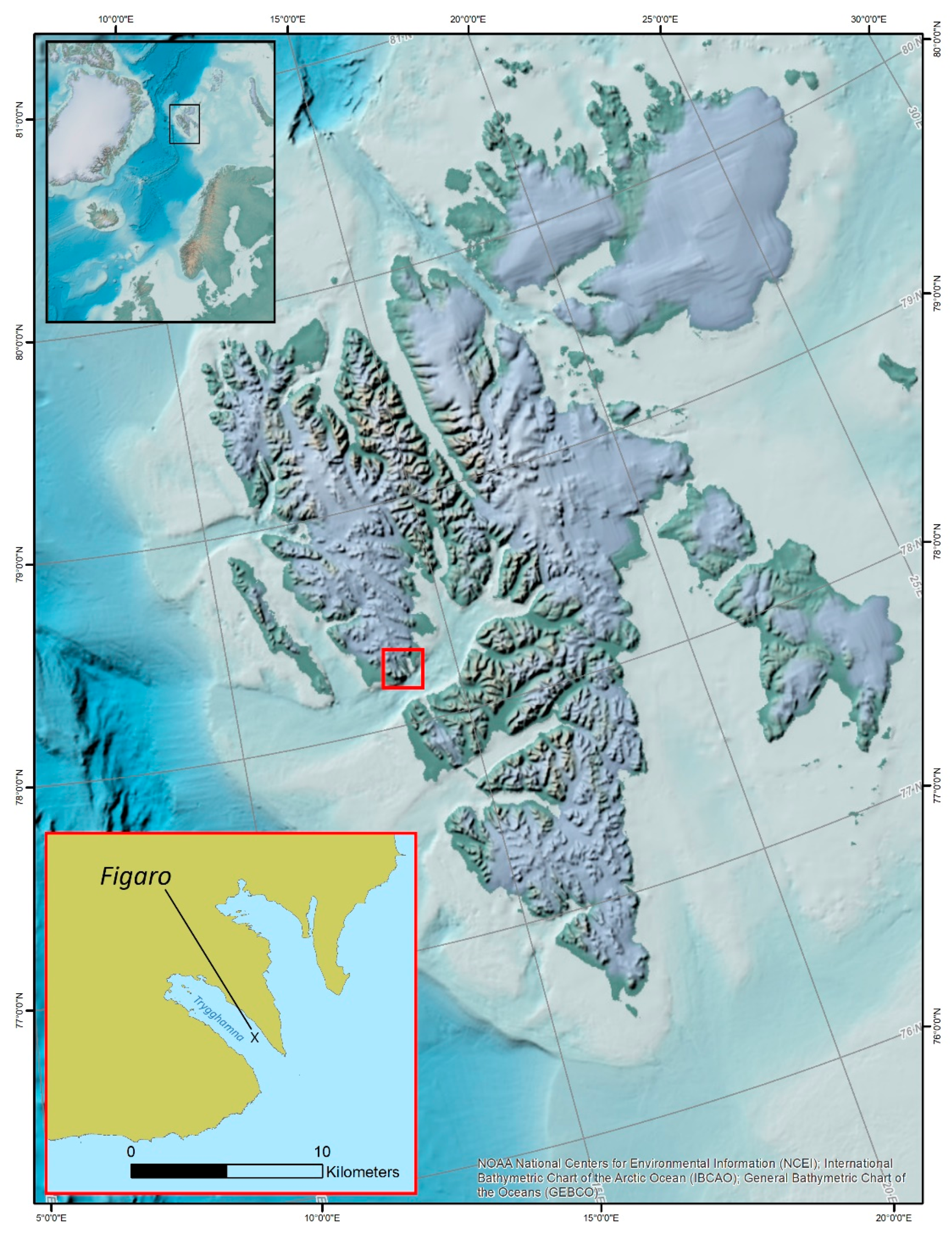
2.1. Study Area

The wreck site is located in Trygghamna (78°14.440′N 13°50.021′E), a small fjord on the north side of the inlet to Isfjorden, Svalbard (Figure 1). Four glaciers have meltwater runoffs into the fjord, which has a maximum depth of 126 m. The fjord is surrounded by mountain ridges and has been favored as a safe anchorage by whalers and seafarers through history, hence the name Trygghamna—Safe haven—in Norwegian. The wreck rests at 30–40 m water depth on a shallow shelf-like area on the east side of the fjord. The seafloor is covered in fine-grained sediment, which is typical for fjords with glacial runoffs and moderate exposure to currents and rough sea states.

2.2. Autonomous Underwater Vehicle (AUV) and Mini-Remotely Operated Vehicle (ROV) Survey 2015

The initial survey of the wreck site was conducted in early September 2015 using a REMUS 100 autonomous underwater vehicle (AUV; Hydroid Inc., Pocasset, USA) equipped with a 900 kHz Marine Sonic sidescan sonar (SSS; Marine Sonic Technology Ltd., Yorktown, USA) to acquire seafloor imagery from four consecutive passes of the wreck site. Access to multibeam echo sounding (MBES) data from the Norwegian Hydrographic Service provided position and basic orientation of the wreck for AUV path planning. Two acoustic beacons were positioned at known positions set in the mission plan, to function as a long baseline (LBL) positioning system to ensure precise vehicle navigation. The SSS images were downloaded immediately after the mission, and clearly showed that the wreck was structurally intact to a large degree, with several elements from sail rigging and whale oil processing, scattered on the seafloor near the wreck.
Directly following the AUV operation, a Seabotix LBV 200 mini-remotely operated vehicle (ROV; Teledyne Technologies Inc., Thousand Oaks, USA) was deployed to visually inspect and record the wreck. In addition to a standard definition (SD; < 720p) camera with an overlay showing depth, position and heading for navigation, the mini-ROV was equipped with an ultra-short baseline (USBL) positioning system (receiving global navigation satellite system—GNSS—data from the surface vehicle) and a scanning sonar to guide navigation on the wreck site during reduced visibility conditions. A high-definition (HD) camera with zoom and tilt functionality was used to perform recordings of objects and features of interest.
The real-time position of the ROV could be monitored on a computer screen showing a bathymetric model of the wreck based on MBES data. Juxtaposing this display with the scanning sonar display and the recently acquired SSS images, it was possible to navigate between salient features within the complex spatial context of the wreck site. During the summer, fjords on Svalbard typically have turbid waters due to high phyto- and zooplankton biomass, and inorganic suspended matter mainly provided by freshwater runoff from glaciers and melting snow. The video quality was therefore dependent on close-range recording, with detail losses occurring already at 1 m distance. Maneuvering at seafloor altitudes <1 m often resulted in thrusters whirling up fine-grained sediment, impairing video quality. During navigation it was often necessary to turn off the ROV lamps completely, leaving the pilot entirely dependent on illumination provided by ambient sunlight. Consequently, overview imagery of the wreck site was difficult to obtain. Due to the small size and weight of the ROV, it was, however, possible to perform very close-range inspection of objects and features of interest without optical backscatter from the lamps posing any noteworthy concern. All aforementioned field operations were conducted within a timespan of <12 h. During ROV operations, the AUV was deployed again to do seabed mapping in adjacent areas. No other cultural heritage objects were detected.

2.3. ROV Mapping 2016

Based on the data from the 2015 survey, a full ROV survey of the wreck was planned and conducted as part of a Polar Night Research Cruise with RV Helmer Hanssen (UiT—The Arctic University of Norway) in January 2016. For the survey, Minerva, a Subfighter 7500 medium class (485 kg) ROV (Sperre AS, Notodden, Norway), was equipped with an HD video camera, stereo cameras for the photogrammetry, and an underwater hyperspectral imager. A graphical user interface (GUI) for logging scientific observations (Urd) was used to tag archaeological and biological observations with a timestamped position. A forward-facing HD video camera was used for navigation by the pilots and for real-time observation of possible objects of interest by the scientists. A full recording of the HD video was reviewed together with other sensor data and logged Urd observations during post-mission analysis. The primary objectives of the survey were to acquire images for a full photogrammetric model of the wreck and to acquire underwater hyperspectral imagery for classification of cultural and natural objects of interest.
Minerva was fitted with a dynamic positioning (DP) system [6], to enable precise navigation and maneuvering (e.g., station keeping). A portable hydroacoustic position reference 300 system (HPR300; Kongsberg Gruppen ASA, Kongsberg, Norway) was fixed to a pole and lowered approximately 5 m into the water on the starboard side of RV Helmer Hanssen. Utilizing a USBL modem, the ROV could estimate its position relative to the GNSS position of the ship and pilots could track the ROV position in real-time on a computer showing a map of the wreck site based on the existing MBES and SSS data. Due to the size and complexity of the wreck site, a detailed mission plan with transects to ensure full data coverage had been prepared considering stereo camera field of view (FOV) and the required close range to the wreck due to turbidity. However, since RV Helmer Hanssen did not have a DP system, the ship had to lie on anchor at a safe distance (150–200 m) from the Figaro to ensure that the anchor chain did not come near the wreck site. As the ship moved with the tide, the USBL coverage from the ship to the ROV experienced frequent intervals with loss of contact or severe positioning errors. For extensive periods the pilots could not navigate based on the USBL positioning system and had to rely exclusively on visual navigation. Consequently, it was difficult to assess whether full coverage was obtained, and a strategy based on data acquisition redundancy was adopted to avoid spatial gaps in the stereo camera imaging of the wreck site. Particular attention had to be given to the ROV tether to avoid entanglement or disturbance of the wreck site, and to avoid collisions between the ROV and protruding parts of the wreck during lateral transects (the ROV navigating sideways) conducted for the purpose of recording the broadsides of the wreck. Lack of high-quality positioning also affected the full utilization of Urd and the post-mission photogrammetric modeling pipeline.

2.4. Photogrammetry Data Acquisition

Minerva was equipped with two Allied Vision GC1380C cameras (Allied Vision GmbH, Stradtroda, Germany) spaced 31.5 cm apart in a 45° forward-facing stereo camera setup. Each stereo camera had a resolution of 1360 × 1024 pixels. With steady maneuvering of the ROV at close range to the wreck and image capture set to 0.5 frames per second (fps), we aimed for a 60% overlap between sequential image pairs to ensure a continuous and consistent model during photogrammetric post-processing. A detailed description of the setup and acquisition method can be found in Nornes et al., 2015 [7]. For salient features with vertical faces, like boilers and vats, it was difficult to ensure that images were captured from all angles while simultaneously following systematic transects. Without the ability to monitor the ROV transects on a map, coverage control largely depended on the ability of the pilot and researcher to remember and recognize objects and features. The human capacity for spatial and contextual awareness and orientation decreased after hours of intense focus and concentration, resulting in repeated transects for some areas and under-coverage for others. A total of 33,228 images were acquired during 6:30 h of surveying on January 12th and 4 h of surveying on January 17th. The cameras were mounted on the ROV frame, and maneuvering safety constrained the ability to perform close-up recording of parts of the wreck site, especially around features with overhang or other confined spaces. As there is no ambient light during the polar night, two forward-facing hydrargyrum medium-arc iodide (HMI) lamps and two downward-facing halogen lamps were the only sources of illumination. In January, water temperatures in Svalbard are <4 °C, and visibility is generally good due to the absence of freshwater runoff from land. However, increased turbidity was sometimes caused by thrusters resuspending sediment when navigating at low seafloor altitudes or when the tidal current brought sediment from RV Helmer Hanssen’s anchor chain into the water masses over the wreck area, resulting in poor image quality. With the seafloor altitude mostly kept at 1–1.5 m, the camera FOV of the wreck site was typically between 1 m and 2 m wide. With limited time available for data acquisition, areas within the hull of the wreck were prioritized.

2.5. Photogrammetry Data Processing

During the last decade, photogrammetric surveying has become a well-established method in underwater archaeology and the processing principles have been published in depth in works such as Drap, 2012 [8] and Yamafune, 2016 [9], and for underwater robotic surveys, in particular by Johnson Roberson et al., 2010 [10]. A description of the processing pipeline used in this survey is described in Nornes, 2018 [11]. A Contrast Limited Adaptive Histogram Equation (CLAHE) algorithm was used to perform initial color correction of all images. The procedure enhances feature distinction, mitigates vignetting effects due to unevenly distributed light fields and reduces image size. The navigational issues described above, combined with turbidity and the relatively low resolution of the cameras, resulted in suboptimal image quality for certain areas of the wreck site, which in turn impeded the ability of the photogrammetry software (Agisoft Photoscan; Agisoft LLC., St. Petersburg, Russia) to carry out feature-based matching of overlapping photos. A considerable number of hours were spent on manual tagging of prominent features in images, and iterative processing of camera positions had to be done to close the loops for a consistent and spatially coherent geometric model of the wreck. A hard-learned lesson for an archaeologist was that pronounced features suitable as markers for registration of images often could belong to biological organisms that over a period of hours were not spatially inert. This became more apparent when the second set of images acquired five days later were introduced to the model. Geographic positions of prominent features in the fore and aft area of the wreck that were identified in the MBES data set were used to geo-reference the model. As the positioning system could not be relied on to deliver precise navigational data for the ROV, and hence neither the camera planes for all images, obtaining accurate error estimates for the model and subsequent orthophotos was not possible.

2.6. Acquisition of Underwater Hyperspectral Imagery

During the process of collecting stereo camera data for the wreck site photogrammetry on January 12th 2016, an underwater hyperspectral imaging (UHI) transect from the top of the Figaro wreck site was also acquired. UHI represents a high-spectral-resolution optical mapping technique (each recorded image pixel contains a contiguous light spectrum as opposed to a regular RGB—red, green, blue—value) that over the past decade has emerged as a promising seafloor mapping tool [12,13,14,15]. The hyperspectral imagery was captured using the underwater hyperspectral imager UHI-2 (2nd generation underwater hyperspectral imager; Ecotone AS, Trondheim, Norway). UHI-2 is a waterproof push-broom scanner that captures hyperspectral pixel rows through an 8-mm fore lens, by means of a scientific complementary metal-oxide-semiconductor (sCMOS) camera sensor with a 16-bit radiometric resolution (dynamic range). The imager’s FOV in the across- and along-track directions is 60° and 0.4°, respectively, and its maximum spatial resolution is 1600 across-track pixels. Spectrally, UHI-2 covers the range of 380–800 nm at a maximum resolution of 0.5 nm.
To record underwater hyperspectral imagery, UHI-2 was deployed on the port side of Minerva in a nadir viewing position, with its across-track FOV oriented perpendicularly to the ROV’s heading. Illumination for the image acquisition was provided by two downward-facing, 250-W halogen lamps mounted 35 cm aft and fore of the imager. Once the ROV had been deployed, UHI-2 was controlled remotely from RV Helmer Hanssen using the software SpectralDAQ (Specim, Spectral Imaging Ltd., Oulu, Finland). To increase signal-to-noise ratio and enhance the processability of the hyperspectral data products, spatial resolution was binned down from 1600 to 800 across-track pixels per exposure. Similarly, the spectral resolution was reduced from 0.5 to 2 nm. The UHI transect was recorded at a frame rate of 16 Hz, using an exposure time of 25 ms. During the image acquisition, Minerva was manually maneuvered in a line across the wreck site at a speed of approximately 25 cm s−1. The seafloor altitude varied between 0.5 m and 1.2 m. The recorded UHI transect was stored as a RAW file on the internal hard drive of UHI-2 and exported for processing upon survey completion.

2.7. Processing of Underwater Hyperspectral Imagery

The wreck site UHI transect was processed using the software application ENVI (Environment for Visualizing Images, v. 5.5; Harris Geospatial Solutions Inc., Boulder, USA). Initially, the UHI data were converted from digital counts into upwelling spectral radiance (W m2 sr−1 nm−1) to remove noise and influences inherent to the sensor. This procedure was carried out using the ENVI plug-in “Hypermap” from Ecotone AS (Trondheim, Norway). Following radiance conversion, the next step is typically obtaining absolute reflectance. However, conversion into absolute reflectance requires accounting for underwater light beam attenuation based on the water column’s inherent optical properties (IOPs) and the properties of the light source(s), neither of which were known in sufficient detail. Consequently, radiance was converted into internal average relative reflectance (IARR) instead. In an IARR conversion, all pixel spectra are divided by the mean spectrum of the full scene [16], which yields a result that is comparable to absolute reflectance. It is worth noting that neither reflectance nor IARR is a prerequisite for conducting spectral classification. The IARR conversion in the current study was only performed to facilitate the interpretation of the UHI transect and its constituent objects of interest. Prior to the IARR conversion, the spectral illumination in the radiance-converted transect was normalized both across- and along-track to account for constant geometric differences in the light field generated by the halogen lamps (across-track) and slight variations in seafloor altitude (along-track). The normalization was carried out in ENVI using the multiplicative correction method of the function “Cross-Track Illumination Correction” with 5th degree polynomials. The resulting transect was subsequently converted into IARR using ENVI’s “IAR Reflectance Correction” tool. The final step that was carried out before spectral classification was georeferencing of the IARR-converted transect. Georeferencing was performed in Hypermap based on 86 time-stamped ROV positions extracted from the Figaro photogrammetry model. Each time-stamped position featured a Structure-from-Motion-based (SfM) pose of the vehicle with values for latitude, longitude, pitch, roll, heading, depth, and seafloor altitude, and the IARR data were georeferenced at 0.5-cm spatial resolution.

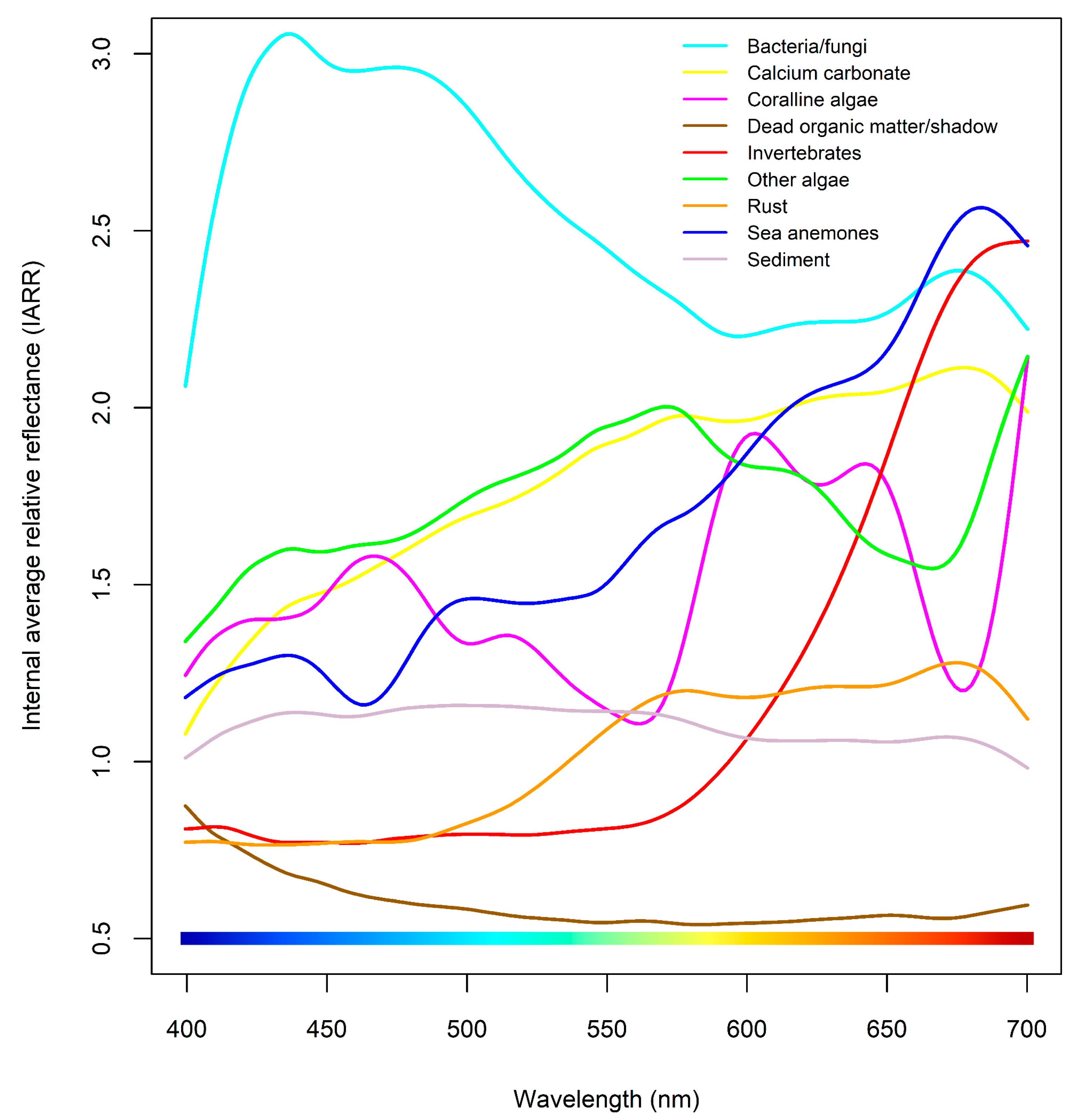
2.8. Supervised Classification of Underwater Hyperspectral Imagery

Supervised classification of the georeferenced IARR data was carried out using a combination of the software application ENVI and the software environment R (v. 3.5; R Foundation for Statistical Computing, Vienna, Austria). For the classification procedure, the IARR data were spectrally subset to the range of 400–700 nm (a total of 156 bands). This was done to eliminate noisy bands where the ROV lamps provided insufficient lighting. To acquire training data for the supervised classification, spectral endmembers (spectrally pure pixels) were identified in the georeferenced transect using ENVI’s “Minimum Noise Fraction (MNF) Rotation” (modified from [17]) followed by the “Pixel Purity Index (PPI)” function. The MNF Rotation can be considered a double principal component transformation, where the first transformation decorrelates and rescales (“whitens”) the noise in the dataset and the second transformation displays the inherent dimensionality of the dataset. In the current study, the first eight MNF bands were found to yield coherent transect images. Consequently, these bands were chosen as input for the PPI analysis. The PPI function locates the purest or most extreme pixels by projecting n-dimensional scatterplots of the dataset onto random unit vectors a predefined number of times and counting each time a given pixel is marked as extreme. Pixels frequently counted as extreme are assumed to belong to spectrally distinct classes. By applying the PPI and interpreting the resulting pixel purity image in context with the georeferenced IARR transect, nine spectral classes were identified. Six of the identified classes were assumed to be biofouling spectral classes, whereas the remaining three were assumed to be non-biofouling. For each class, pixel endmembers highlighted by the pixel purity image were extracted from the IARR transect to be used as training data for supervised classification. Table 1 presents the assumed identities of the nine different spectral classes and the number of training pixels obtained for each of them, while Figure 2 shows each class’ mean IARR signature.
For the supervised classification, a support vector machine (SVM) classifier with a radial basis function (RBF) kernel was selected. By using vector-defined decision surfaces based on the provided training data, SVM maximizes the margins between different classes. The SVM algorithm was chosen due to its ability to handle complex data [18,19] and its previous performances on UHI datasets [12,13,15], whereas the RBF kernel was chosen based on its robustness [20,21]. Supervised classification by means of an RBF-SVM classifier requires parameters γ (kernel width) and C (regularization degree) to be specified (Kavzoglu and Colkesen, 2009) [20]. To determine the optimal γ and C values for RBF-SVM classification of the current dataset, a grid search cross-validation was performed on the obtained training data (third column of Table 1) in the software environment R, using the package “e1071” [22]. The optimal parameter values were determined using ten-fold cross-validation, which found that a γ of 0.0001 in combination with a C of 10,000 yielded the best classification model (99.43% cross-validation accuracy). To further verify the validity of the model, a test set validation was also carried out by applying the model to the pixel test set shown in the fourth column of Table 1. The test set validation showed an overall classification accuracy of 93% and a Kappa coefficient of 0.93, suggesting strong agreement between the model and reality [23]. Class-specific classification accuracies from the test set validation are shown in the Table 2 confusion matrix, which class by class assesses the agreement between predicted and true values. Table 2 also shows class-specific estimates of both producer accuracy and user accuracy. The former is calculated by dividing the number of correctly classified pixels within a class by the true number of pixels known to be that class, whereas the latter is calculated by dividing the number of correctly classified within a class by the number of pixels predicted to be that class by the given classifier. The optimized RBF-SVM classification model was ultimately applied to the entire georeferenced IARR transect in ENVI, and the results were exported to ArcMap (v. 10.6; Esri Inc., Redlands, USA) for visualization and interpretation.
Within the transect, three different archaeological substrate types were identified: “metal wires/pipes”, “protruding wood” (wood protruding significantly from the surrounding seafloor), and “receding wood” (wood at the same level as the surrounding seafloor). This process was aided by comparing the UHI transect to the photogrammetry model of the Figaro. The remaining pixels in the transect were assigned to the generalized substrate type “remaining transect”. Using defined pixel regions of interest (ROIs) corresponding to each substrate type (Appendix A, Figure A1), substrate-specific areal coverage (%) was estimated for all spectral classes based on the RBF-SVM classification results. These estimates are presented in the Results section, along with the equivalent estimate for the entire transect combined. Finally, the proportions of biofouling and non-biofouling pixels were estimated for each substrate type. These proportions were subsequently compared statistically in the software environment R using chi-squared (χ2) testing with Yates’ continuity correction. This was done to identify potential differences between archaeological substrate types and the generalized remaining transect.

3. Results

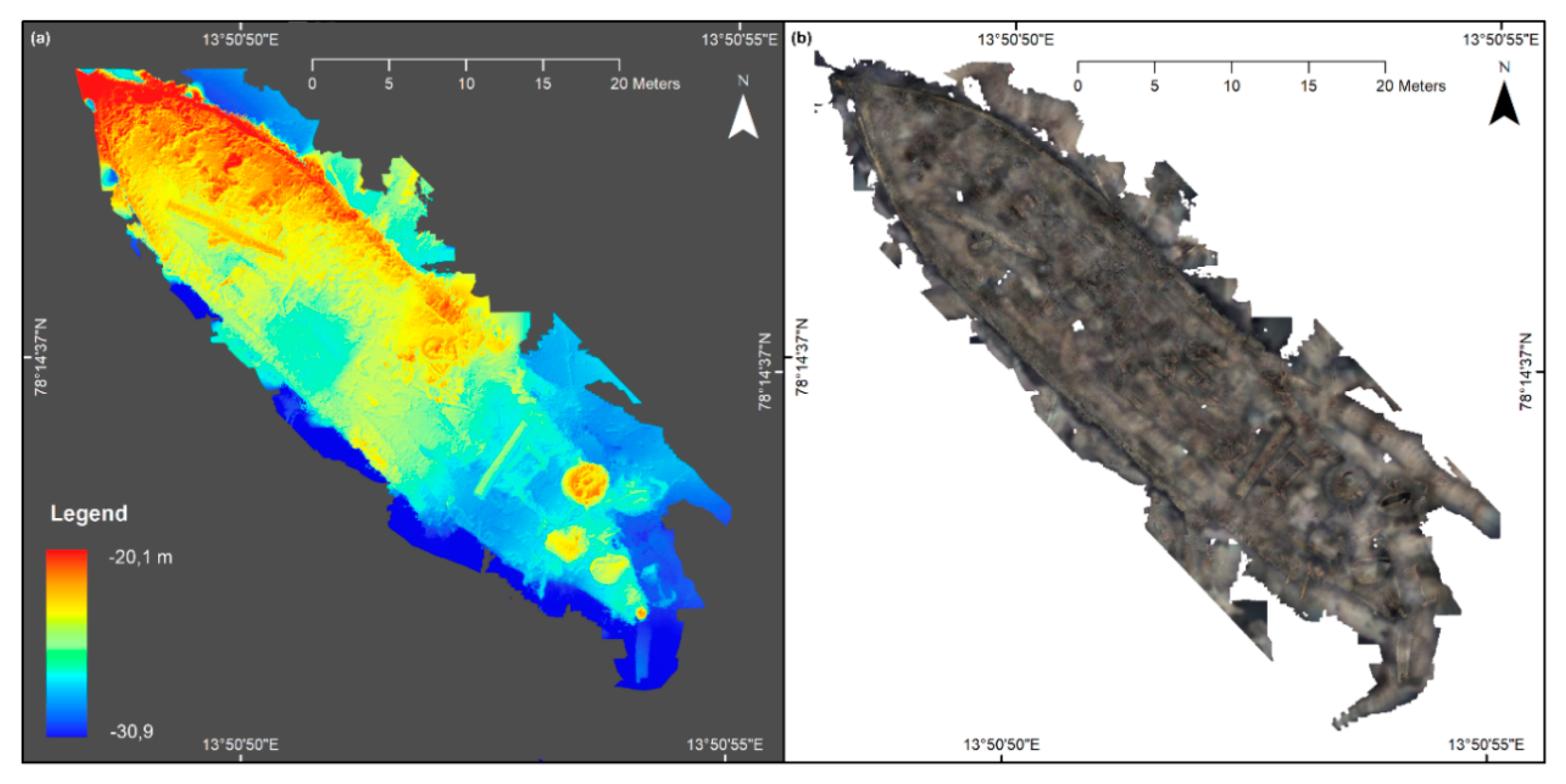
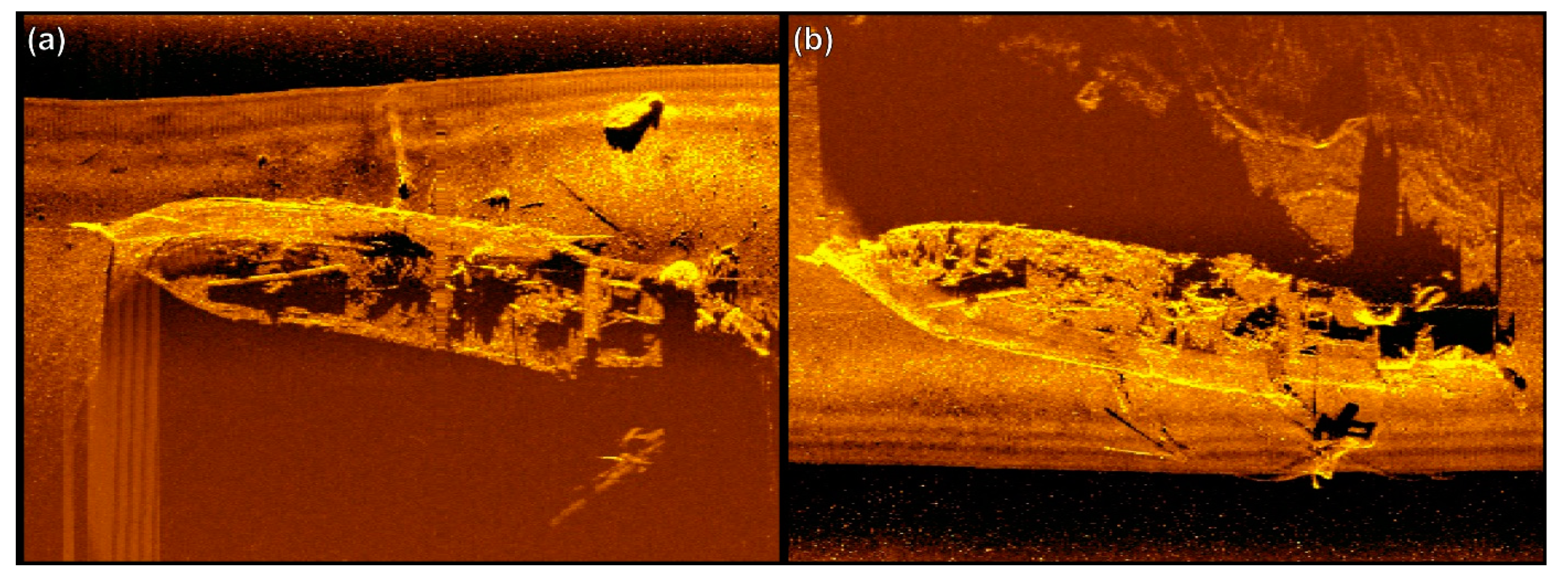
3.1. AUV and Mini-ROV 2015 Results

The SSS imagery (Figure 3) showed the wreck site with an apparently structurally intact hull resting upright on the keel on the slightly sloping seafloor. Several boilers were visible inside or in close proximity to the aft section of the wreck. Additionally, two chimneys were distinctly visible, attesting that the ship had been fitted for modernized (by contemporary standards) whale blubber processing. Other salient features that could be seen in the SSS imagery were an anchor chain on the starboard side, the rudder lying flat on the seafloor next to the stern post, and parts of the rigging on the seafloor outside the port side of the wreck. Comparing imagery from both sides of the wreck enhanced our ability to interpret both echo intensity and shadows in a complementary manner, making it possible to e.g., discern the shape and extent of an upright standing boiler in the starboard aft area. Multi-view fusion as described in Ødegård et al., 2018 [24] was not possible due to spatial inconsistencies, but the added value of multiple aspects was apparent when considering the details in the starboard forward section that were only visible in one of the images. The image from the port-side pass (Figure 3b) showed a shadow of the wreck site’s vertical profile. It indicated an increased hull disintegration towards the aft area, though one had to consider that the sloping area on the starboard side caused exaggerated shadow length towards the forward section.
In total, 2:34 h of HD ROV-video of the wreck site were acquired. The different parts of the hull and a number of objects were inspected at close range for identification and to assess the state of preservation. The ship’s hull was fitted with copper sheathing that was visible on all inspected remaining hull structures on both sides of the wreck, and we could infer that the wreck was preserved to the waterline or slightly above. A slight outward curvature (peeling) of the upper row of copper plates could be interpreted as a result of fire or high temperatures, congruent with the Figaro burning before sinking. At selected areas, close-range inspection of the ceiling (the planking that separates the cargo from the hull itself) was carried out to look for evidence of fire. No traces of charring could be identified, but significant biofouling along much of the remaining gunwale left the answer to this question inconclusive. Areas of exposed wood seemed to be well preserved with none of the characteristic signs of destruction caused by shipworm (wood-boring mollusks in the families Teredinidae and Xylophagaidae). However, by zooming in on one piece of ceiling timber we could clearly observe evidence of gribble (wood-boring crustaceans in the family Limnoriidae) attack (Figure 4).
The inside of the hull was covered with what appeared to be a thick layer of dead barnacles (crustaceans in the infraclass Cirripedia) and other calcareous shell remains mixed with fine-grained sediment, suggesting relatively high levels of biological activity on the wreck site. A number of well-preserved wooden barrels arranged in rows (indicating they were located in the cargo hold) showed no evidence of gribble or other wood-boring organisms (Figure 5). Steam boilers, cooking vats, and other metal objects were all largely covered with barnacles. Spectrally conspicuous red coralline algae (Rhodophyta) also made considerable contributions to the observed biofouling community. An exception was the copper sheathing and brass bolts extruding from timbers, which showed little or no signs of biofouling or growth. The latter is consistent with copper being a well-known biofouling deterrent [25].
Based on historical records and the analysis of SSS images and ROV video, we could confidently identify the wreck as the Figaro, a Norwegian whaling ship that accidentally caught fire and sank in Trygghamna in 1908. The Figaro was a barque built at the Joh. C. Tecklenborg shipyard in Geestemünde, Germany in 1879. It was the last wooden barque to be built at that shipyard, and measured 1044 grt, 985 nrt, L: 54.4 m; B: 10.8 m; D: 6.8 m. In 1902, the ship was acquired by a Norwegian company, rebuilt and put into service as a floating whalery in 1904. It was among the first ships fitted with equipment for industrial processing of whale blubber and served for four years in Spitsbergen in the final phase of commercial whaling in the European Arctic. The ship functioned as a stationary factory base for one or two smaller steam-powered vessels that brought whales in from the hunting grounds off the Svalbard coast. After flensing and boiling, processed oil was put on caskets and stored in the cargo hold for transport back to Norway at the end of each season.

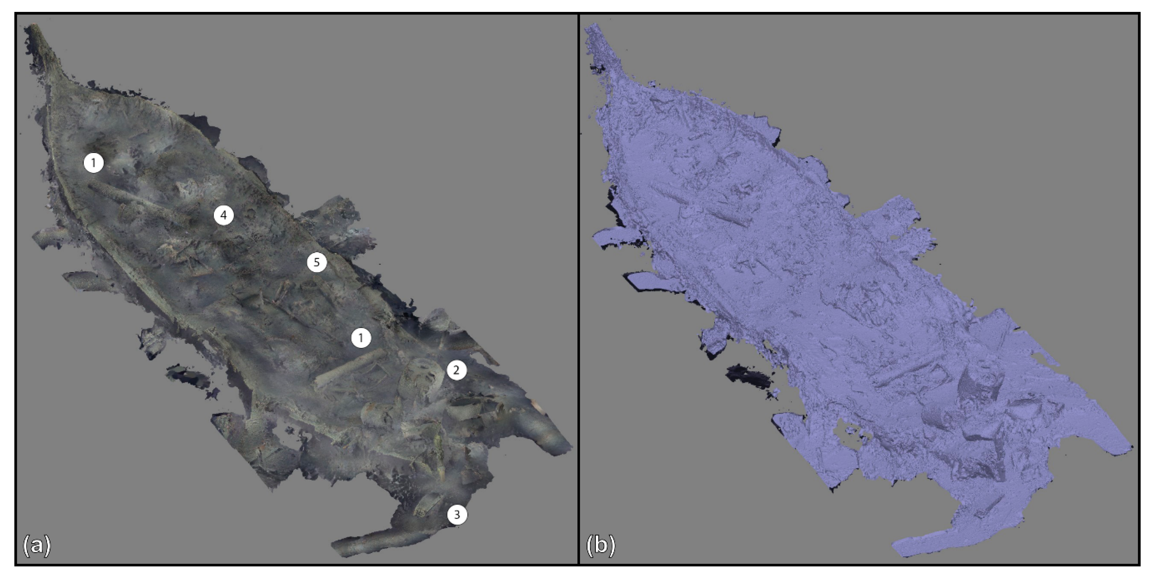
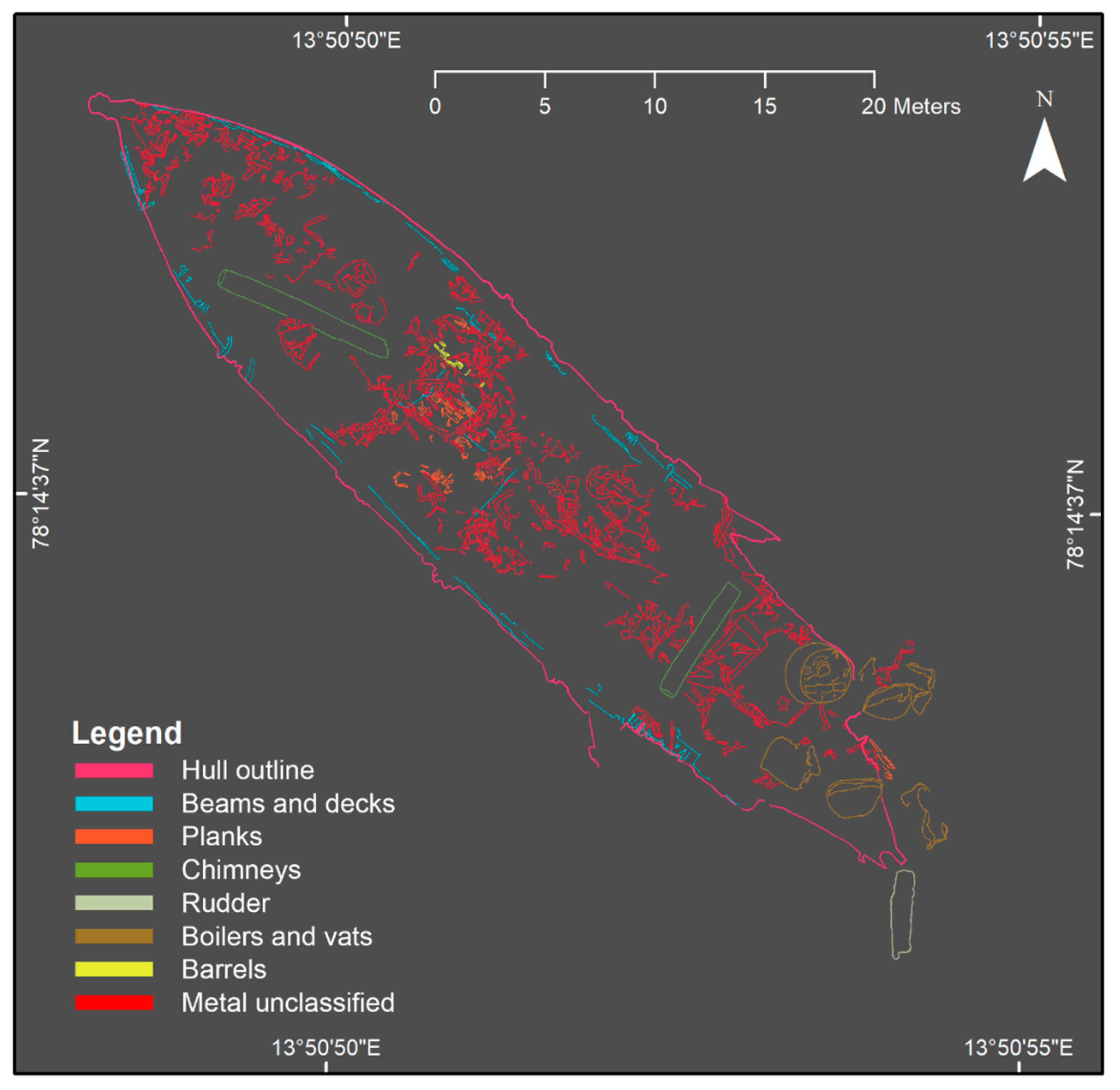
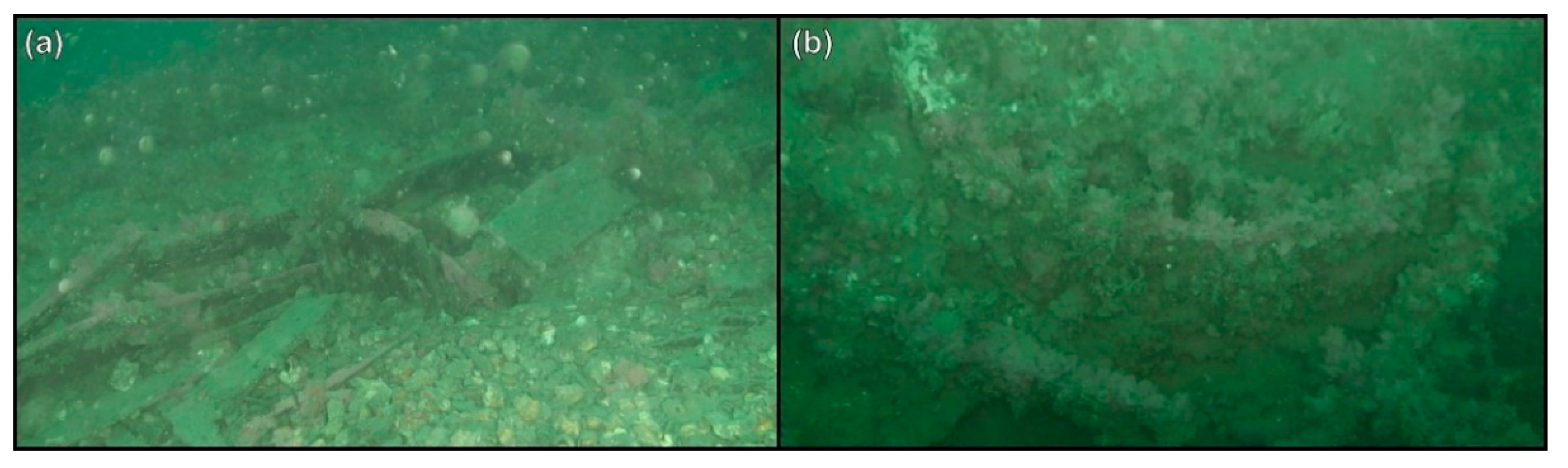
3.2. ROV 2016 Photogrammetry Results

The full photogrammetric mapping of the wreck site conducted during the 2016 Polar Night Cruise was planned based on the results of the 2015 survey. The inherent optical properties of the water column that impaired image quality in September 2015, were significantly reduced in January 2016, as can be seen by comparing Figure 5 and Figure 6.
The full 3D-model of the wreck site showed varying degrees of consistency and level of detail, mostly due to poorer coverage or image quality in some areas. Particularly, the shaded areas where the outside of the hull meets the seafloor had gaps due to insufficient data for a continuous model. In addition to the 3D model that could be viewed in the Agisoft Photoscan software as textured or solid (Figure 7), a high-resolution digital elevation model (DEM) model and an orthophoto were the main products for analysis and interpretation (Figure 8). The bow section was most structurally intact, with the stem post standing 9 m proud of the ambient seafloor. The rudder post stood 3.6 m above the seafloor surrounding the aft section of the vessel. The wreck measured 51 m from stem to stern, and 11 m wide. An archaeological site plan of the wreck was drawn as classified layers on top of the orthophoto (Figure 9). Distinct objects and features, e.g., boilers and chimneys, were easy to identify and delimit in the orthophoto and hence transferred to the site plan with high relative accuracy. Discrimination between barrels and other planks or pieces of wood was not apparent, and classification had to be based on spatial context. Classification of metal objects was challenging due to their complex distribution, but also the considerable layers of biofouling obscuring their original shape. This class should therefore be considered somewhat uncertain. Still images, the hillshaded DEM and HD video recordings were used to aid classification in areas where the orthophoto had insufficient levels of detail or quality. A bit surprisingly, no bottles, ceramics, or bricks could be seen on the wreck site.

3.2.1. Wood

Wood was visible along the gunwales, mainly in parts of the frames and ceilings. Biofouling and sediment occluded most prominent features from detailed inspection, but observable exposed surfaces were seemingly intact and well preserved. Remains of the rig and other wooden objects deposited on the seafloor outside the wreck appeared to be in similar condition. In some areas, surfaces that likely were part of deck planks were visible, indicating that the inner structure of the wreck was compressed but not completely collapsed. A number of barrels could easily be identified due to characteristic rows of barrel lids standing upright in situ. Other concentrations and scatterings of planks could be observed, but not classified. Exposed wood in the rudderpost showed signs of deterioration that could have been caused by shipworm (Figure 10a). The general assessment was that wood was well preserved all over the wreck site.

3.2.2. Metal

The only metal that could be identified as part of the ship structure itself was the copper sheathing covering the hull, rudderpost and rudder, and a number of bolts protruding from frames and ceiling. Neither the sheathing nor the bolts were biofouled to a large extent. The bolts in fact appeared to be completely bare, which made them particularly easy to identify. One chimney, at least two boilers, and 4–5 vats were observed in the aft section of the wreck. An additional chimney was found in the fore section, and another vat was detected approximately 30 m outside the starboard side of the wreck. All these metal objects were covered with biofouling organisms (mainly barnacles and coralline algae). The two boilers had exposed patches with rust (Figure 10b). Metal objects were ubiquitous inside the wreck, but with concentrations that indicated stations with machinery or constructions. Metal frames, wheels and pulleys, and large amounts of what appeared to be wire were congruent with activities related to mechanized whale processing. Typically, all metal objects were covered with crust-like layers of biofouling organisms (as can be seen in Figure 6b), and except for the two boilers, no exposed metal surfaces could be observed. Additionally, except for a few patches of rust-colored sediment next to metal objects, there was no evidence of substantial corrosion or oxidized concretizations that are typical for saltwater wreck sites.

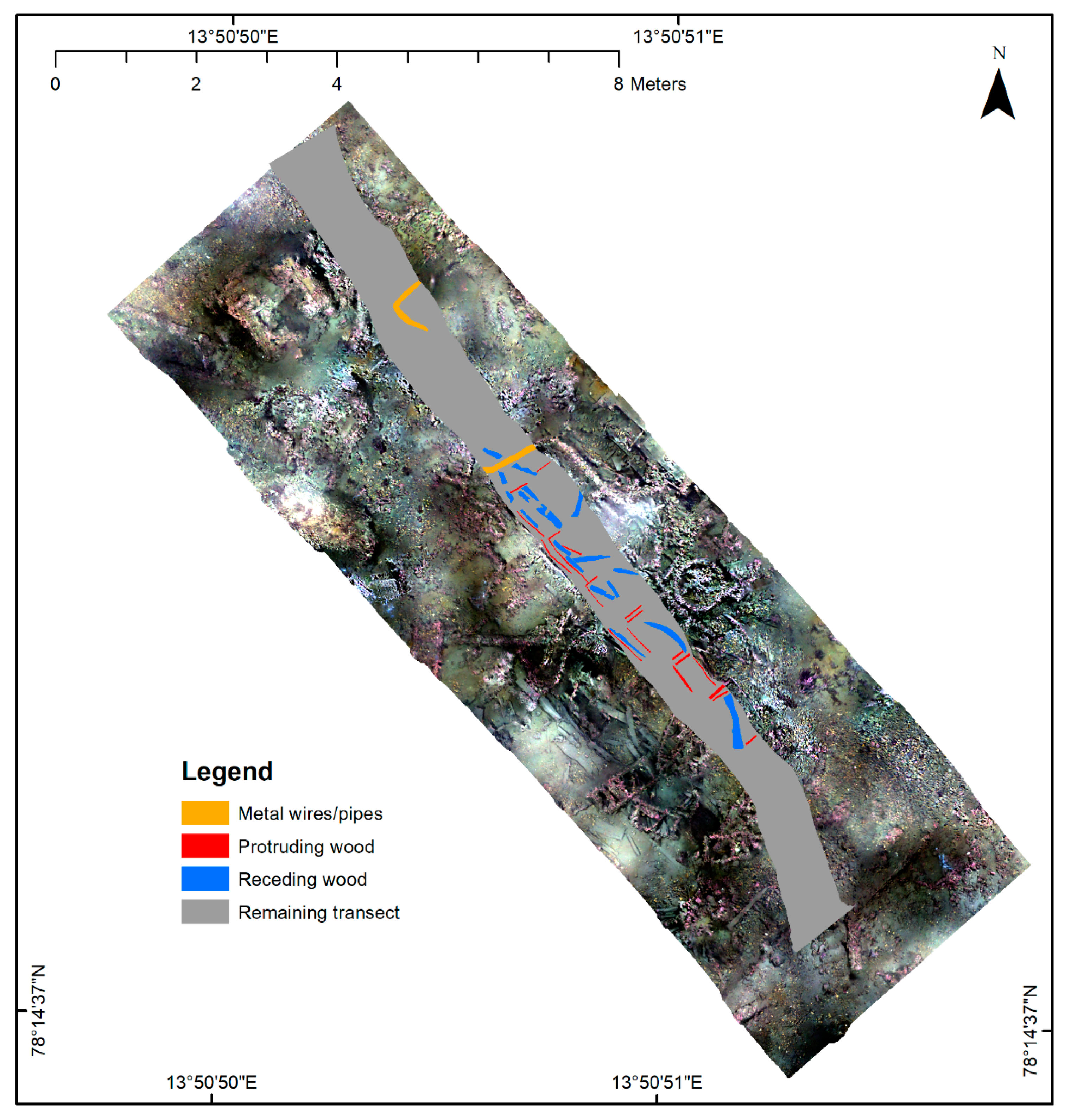
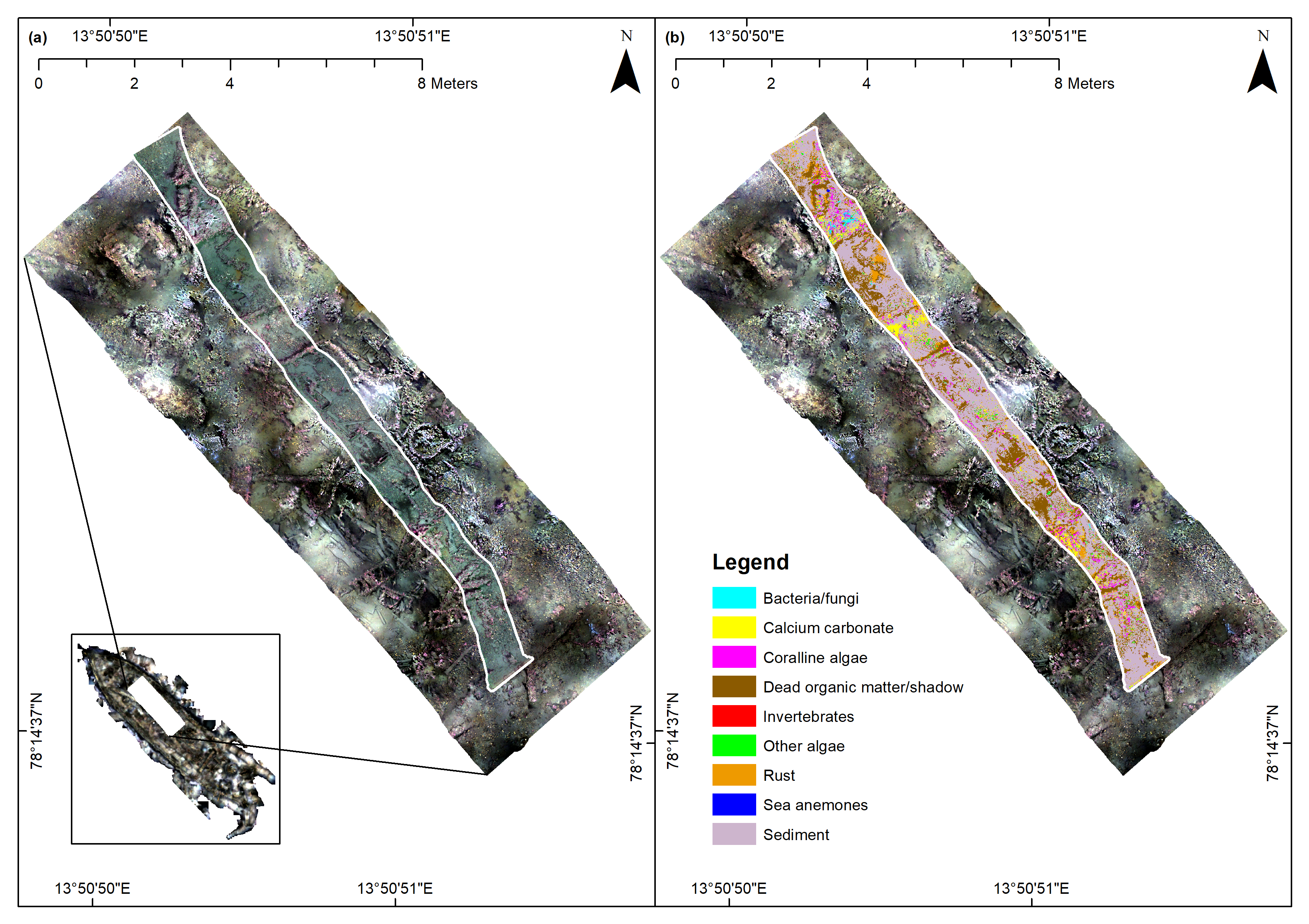
3.3. ROV 2016 Underwater Hyperspectral Imaging (UHI) Results

Figure 11a shows an RGB representation of the IARR-converted and georeferenced UHI transect, in context with the photogrammetric 3D model of the Figaro wreck. The transect covered an area of 14.65 m2 and appeared highly consistent with the Figaro 3D model spatially. Results from the corresponding SVM classification are shown in Figure 11b. Taking the full transect into account, sediment and dead organic matter/shadow were estimated to be the most abundant spectral classes. The spectral classes rust (mostly in the form of rust-colored sediment), calcium carbonate, and coralline algae were also estimated to be present in substantial amounts. Specific areal coverage estimates for all spectral classes are shown in Figure 12. In addition to showing the estimates for the full transect, Figure 12 shows equivalent estimates for transect regions corresponding to metal wires/pipes, protruding wood, receding wood and the remaining transect. The estimated levels of biofouling in all the assessed substrate categories and the full transect are shown in Table 3. Of the archaeological substrate types, receding wood was found to support significantly lower levels of biofouling than the remaining transect, whereas metal wires/pipes and protruding wood were found to support significantly higher levels (Table 3). The patterns observed in Figure 12 and Table 3 and their associated implications are further examined in the Discussion section.

4. Discussion

4.1. Use of Underwater Robotics and Sensors for Mapping a Wreck Site

Due to the location of the Figaro in a remote and harsh environment, the strategic choice to utilize underwater sensor-carrying robots for investigation and mapping was appropriate. Guided by the principles in Ødegård et al., 2016 [26], deployments of different vehicles and sensors were done in successive missions with data and information consecutively being used during each step of planning, acquisition and processing (Figure 13). The reduced functionality of the acoustic positioning system had negative consequences for navigation and data registration and emphasized the importance of human-in-the-loop knowledge and preparation to ensure operational success even in a fully “robotized” archaeological survey. Based on the aggregated results from two surveys of relatively short duration, it was possible to successfully delimit the underwater cultural heritage site, identify the wreck as the Figaro, map main features of the wreck site and assess the wreck’s state of preservation for future management decisions. In addition to the scientific data gathered for archaeological and biological analysis and interpretation, valuable operational experience was gained for future surveys utilizing remote sensing technologies in complex environments.
The presented pipeline from image acquisition, via reconstructed geometry, to site plan is cumbersome, to some degree eclectic when it comes to tools and methods, and prone to introduction of uncertainty both in processing and interpretation. As discussed by Drap et al., 2019 [27], the selected approach required a combination of automatic data processing and archaeological knowledge to produce information relevant for the stated purpose of the survey. The production of a site plan (Figure 9) mainly based on visualizations derived from the photogrammetric model is a process of qualitative assessment that relies on the archaeologist’s ability to recognize and identify shapes of objects or features and infer continuations of those shapes when their visible representations are obscured by, for example, layers of sediment or extensive biofouling. The inherent attention in archaeological documentation against omitting data or information from the record, must be balanced against the uncertainty of classification that could possibly introduce errors similarly obfuscating analysis and interpretation.
Two main challenges related to the approach presented in this paper, were the lack of ability to perform ground-truthing, and capacity (excessive time consumption) for interpretation. With increased accessibility to deep water wreck sites, enabled by technological development, we can expect more cases were data capture is limited to the constraints of non-intrusive and remote sensing methods. That means that uncertainty in classification that traditionally has been resolved by closer or even tactile examination must be approached with different tools. The use of UHI as a complementary technique for classification based on optical signatures in addition to morphology could enhance the quality of wreck site interpretation and understanding [28]. In addition to classification of archaeological features, as presented in a site plan focusing on cultural context (Figure 9), attention should be given to wrecks as artificial reefs and how biological activity and diversity are intertwined with site constitution and formation processes [29]. Integrating use of UHI in wreck site surveys could provide maps to elucidate their characteristics as marine ecosystems with both cultural and biological properties, facilitating cross- and interdisciplinary research for better understanding and management.

4.2. Data Quality of Underwater Hyperspectral Imagery

The procedure used for UHI data processing in the current study was able to yield satisfactory results both spectrally and spatially. ENVI’s “Cross-track Illumination Correction” function produced a spectrally coherent dataset with no evident light field variation, while the subsequent conversion from upwelling spectral radiance to IARR generated “pseudo reflectance” that in terms of spectral shape closely resembled absolute reflectance. An example that supports the latter claim is the IARR signature of coralline algae in Figure 2, where distinguished dips corresponding to the in vivo absorption maxima of chlorophyll a (438 and 679 nm [30,31]) and R-phycoerythrin (497 and 566 nm [32,33,34]) clearly are present. The georeferenced IARR transect lined up well with the Figaro 3D model (Figure 11a), which implied that the time-stamped navigation data from the photogrammetry model were sufficiently accurate for geospatial positioning of push-broom hyperspectral imagery. It is worth noting that satisfactory georeferencing of the acquired UHI transect would not have been possible without the supplementary ROV positioning information generated through the photogrammetric analysis of the wreck site.
Although the processing pipeline set up a suitable foundation for the ensuing supervised classification, the authors recommend quantification of two additional parameters for future UHI surveys of wreck sites, namely the water column’s in situ spectral attenuation coefficient and the spectral properties of the utilized light source(s). Detailed knowledge of these parameters would, by means of a radiative transfer model (e.g., that of Maritorena et al., 1994 [35]), permit UHI data to be converted into absolute reflectance (as opposed to IARR), which represents a unit that more easily can be compared to findings from other studies and spectral libraries.

4.3. Supervised Classification of Underwater Hyperspectral Imagery

Based on visual interpretation, the SVM classification results appeared consistent with the estimated 93% classification accuracy from the test set validation (Table 2). Table 2 shows class-specific estimates of both producer accuracy and user accuracy. For seven out of nine spectral classes, both producer- and user accuracy was estimated to be ≥ 90%. The least accurate classification results were obtained for the spectral classes invertebrates and sea anemones. For invertebrates, 13 of 20 test set pixels were classified correctly, yielding a producer accuracy of 65%. The remaining seven pixels were classified as sea anemones, which suggests an overlap between the classes. A partial explanation for this finding is likely that sea anemones, although defined as a distinct spectral class in the current study, also are invertebrates. A common characteristic of yellow, orange, red, and brown marine invertebrates (including many sea anemone species) is that their coloration largely can be attributed to contents of carotenoids (e.g., astaxanthin) and carotenoproteins [36]. This implies that even though the exact pigment contents and pigment-protein relationships differ between invertebrate species, certain interspecific similarities with respect to optical signatures can be expected. For the purpose of this study’s supervised classification, the sea anemone spectral class was initially branched off from the invertebrate spectral class based on the two classes’ seemingly different spectral properties (Figure 2). The estimated classification accuracies in Table 2 do, however, suggest a gradual transition between the classes, and for future biological seafloor surveys featuring UHI, the spectral relationship between marine invertebrate species should be further investigated.

4.4. Biofouling Analysis

A central objective of the wreck site UHI analysis was to investigate the degree to which different marine archaeological materials and artifacts were biofouled, as compared to the surrounding area (the remaining transect). Despite being ubiquitously relevant within fields ranging from marine archaeology to shipping and subsea construction, the complex and intertwined mechanisms that govern the process of biofouling are still largely unresolved. The available knowledge can be considered sparse at best, with a substantial portion originating from studies performed on only a handful of species [25]. The authors would like to point out that considering the generalized nature and small size of the dataset analyzed in the current study, the results presented in Figure 12 and Table 3 need to be treated with caution. With that in mind, we nevertheless believe that certain observed patterns are noteworthy.
Based on the chi-squared tests in Table 3, all archaeological substrate types were found to significantly differ from the remaining transect in terms of biofouling. Two of the three identified archaeological substrates were wooden: protruding wood and receding wood. The final archaeological substrate, metal wires/pipes, was the only substrate to inherently differ from the rest. Factors that are known to affect settlement of biofouling species include intrinsic material properties (e.g., chemical properties), surface texture, and overall surface wettability [25]. By assuming that most woods and metals are comparable in terms of surface wettability (both substrate categories are defined as hydrophilic [37]) and instead emphasizing potential differences in chemical properties and surface texture, metal wires/pipes were expected to stand out the most in terms of biofouling a priori. However, Figure 12 and Table 3 suggest that protruding wood was the substrate that differed the most from the remaining transect (and the full transect). If the six spectral classes bacteria/fungi, calcium carbonate (largely represented by barnacles, based on in situ observations from ROV Minerva), coralline algae, invertebrates, other algae, and sea anemones are assumed to make up the community of biofouling organisms at the Figaro wreck site, protruding wood displayed the highest degree of biofouling (20.01%) by a margin of 3.37 percentage points to the next substrate type on the list (metal wires/pipes). Furthermore, the estimated coverage of biofouling organisms on protruding wood was also 9.28 percentage points higher than that of the remaining transect. Conversely, the degree of biofouling on the other wooden substrate category—receding wood—was only estimated to be 4.29% (6.44 percentage points lower than the estimate for the remaining transect). This suggests that factors besides from the material itself play important roles in determining the degree of biofouling. One such factor could be the degree to which an object protrudes from the seafloor. A strongly protruding object may, for instance, increase a biofouling organism’s exposure to surrounding currents, consequently increasing its access to suspended feed and nutrients. Furthermore, a protruding object will likely trap less sediment than adjacent flat surfaces, which is beneficial to biofouling organisms that are vulnerable to smothering. This reasoning is consistent with findings from a study by Hudon et al., 1983 [38], in which larvae of the barnacle species Balanus crenatus displayed a strong preference for settling sites free of detritus and silt. Since horizontal, flat-surfaced, receding wood supported a substantially smaller biofouling assemblage than the remaining two archaeological substrate types—both of which protruded from the seafloor to a considerable extent—our findings suggest that there exists a positive correlation between object protrusion and wreck site biofouling that needs further elucidation.
On a global scale, as much as 80% of the seafloor is estimated to be comprised of soft-bottom habitats [39], and the surface of soft-bottom habitats typically supports considerably less biomass than that of comparable hard-bottom habitats [25]. The latter is exemplified by the positive effects artificial reef structures submerged in homogenous soft-bottom environments have on biological community recruitment and subsequent biomass production [40,41]. An implication of this and the preceding findings is that hard-surfaced marine archaeological objects that have not completely subsided into the seafloor are likely to support higher biomass than their surrounding areas. Provided that the biological assemblages associated with man-made substrates are composed of sufficiently high densities of spectrally conspicuous organisms (e.g., coralline algae or invertebrates), biofouling could thus serve as an optical cue for detection of novel marine archaeological sites. It needs to be stated that acoustic techniques (e.g., SSS imaging and MBES) are likely to remain the most important tools for this purpose, but for an autonomous framework—such as that proposed by Ødegård, 2018 [42] —where secondary inspection of acoustically identified targets of interest is necessary, optical methods like UHI and photogrammetry should be considered viable options.

5. Conclusions

The findings presented in the current study showcased the utility of combining different state-of-the-art sensor-carrying robots for assessments of wreck sites in harsh and remote areas with limited accessibility, such as the high Arctic. The SSS-equipped AUV served as an excellent means of getting an initial overview of the survey location, based on which more detailed optical ROV surveys could be planned and carried out. Acoustic and optical sensors provided complementary information, and for similar future studies, both should be regarded as necessary for fully understanding the extent, state and complexity of a given wreck site. Furthermore, a considerable benefit of using AUV and ROV technology for wreck site mapping and investigation was that satisfactory results for research and management could be obtained in a relatively short time, reducing operational costs. However, the utilization of advanced technological methods, as described in this paper, introduced vulnerabilities related to equipment malfunctions and unexpected operational events. Overcoming these contingencies (e.g., loss of positioning) and ensuring operational success therefore required careful planning.
Results from the Figaro particularly highlighted the value of advanced optical mapping techniques in relation to wreck site assessments. The photogrammetry of the wreck for instance yielded a detailed 3D model, based on which major wreck site objects and features could be identified in a site plan—a feat that could not have been accomplished based on acoustic data alone. The UHI data provided an additional level of optical information and served as an interdisciplinary bridge connecting archaeology and biology. Specifically, findings from the UHI analyses revealed a possible positive correlation between object protrusion (from the seafloor) and degree of biofouling, which could be of relevance for future marine archaeological surveys using underwater robotic platforms and sensors.

Author Contributions

Conceptualization, A.A.M., Ø.Ø., S.M.N., M.L. and G.J.; Data curation, A.A.M., Ø.Ø., S.M.N., M.L. and G.J.; Formal analysis, A.A.M., Ø.Ø. and S.M.N.; Funding acquisition, M.L., G.J., A.J.S. and J.B.; Investigation, A.A.M., Ø.Ø., S.M.N., M.L. and G.J.; Methodology, A.A.M., Ø.Ø., S.M.N., M.L. and G.J.; Project administration, M.L., G.J., A.J.S. and J.B.; Resources, M.L., G.J., A.J.S. and J.B.; Software, S.M.N.; Supervision, M.L., G.J. and A.J.S.; Validation, A.A.M., Ø.Ø. and S.M.N.; Visualization, A.A.M., Ø.Ø. and S.M.N.; Writing – original draft, A.A.M. and Ø.Ø.; Writing – review and editing, A.A.M., Ø.Ø., S.M.N., M.L., G.J., A.J.S. and J.B. All authors have read and agreed to the published version of the manuscript.

Funding

This work has been carried out at the Centre for Autonomous Marine Operations and Systems (NTNU AMOS). This work was supported by the Research Council of Norway through the Centres of Excellence funding scheme (grant no. 223254—NTNU AMOS). The work was also partially supported by the Research Council of Norway through the Arctic ABC-D project (grant no. 245923—Arctic ABC-D).

Acknowledgments

The authors would like to thank the crew of RV Helmer Hanssen, the engineers at NTNU AUR-Lab and the students involved in the fieldwork during the 2015 UNIS course AT-334 Arctic Marine Measurements Techniques, Operations and Transport.

Conflicts of Interest

The authors declare no conflict of interest. The sponsors had no role in the design, execution, interpretation, or writing of the study.

Appendix A

Figure A1. Regions of interest (ROIs) corresponding to different marine archaeological substrate types in the analyzed underwater hyperspectral imaging (UHI) transect from the Figaro wreck site. The background image is a contrast-enhanced subset of the Figaro orthophoto. The figure was generated in ArcMap (v. 10.6; Esri Inc., Redlands, USA; http://desktop.arcgis.com/en/arcmap/). Projection: UTM 33, Datum: WGS 1984.
Remotesensing 12 00997 g0a1

References

  1. UNESCO. Available online: http://www.unesco.org/new/en/culture/themes/underwater-cultural-heritage/underwater-cultural-heritage/wrecks/ (accessed on 28 February 2020).
  2. Garcia, E.G.; Ragnarsson, S.A.; Steingrimsson, S.A.; Nævestad, D.; Haraldsson, H.; Fosså, J.H.; Tendal, O.S.; Eiríksson, H. Bottom Trawling and Scallop Dredging in the Arctic: Impacts of Fishing on Non-Target Species, Vulnerable Habitats, and Cultural Heritage; Nordic Council of Ministers: Copenhagen, Denmark, 2006. [Google Scholar]
  3. Geiger, J.; Mitchell, A. Franklin’s Lost Ship: The Historic Discovery of HMS Erebus, 1st ed.; HarperCollins Publishers: New York, NY, USA, 2015. [Google Scholar]
  4. Grenier, R.; Bernier, M.-A.; Stevens, W. The Underwater Archaeology of Red Bay: Basque Shipbuilding and Whaling in the 16th Century, 1st ed.; Parks Canada: Halifax, NS, Canada, 2007. [Google Scholar]
  5. Sørensen, A.J.; Ludvigsen, M.; Norgren, P.; Ødegård, Ø.; Cottier, F. Sensor-Carrying Platforms. In POLAR NIGHT Marine Ecology, 1st ed.; Berge, J., Johnsen, G., Cohen, J.H., Eds.; Springer International Publishing: Cham, Switzerland, 2020; pp. 241–275. [Google Scholar]
  6. Sørensen, A.J.; Dukan, F.; Ludvigsen, M.; Fernandes, D.A.; Candeloro, M. Development of Dynamic Positioning and Tracking System for the ROV Minerva. In Further Advances in Unmanned Marine Vehicles, 1st ed.; Roberts, G.N., Sutton, R., Eds.; The Institution of Engineering and Technology: London, UK, 2012; pp. 113–128. [Google Scholar]
  7. Nornes, S.M.; Ludvigsen, M.; Ødegard, Ø.; Sørensen, A.J. Underwater photogrammetric mapping of an intact standing steel wreck with ROV. IFAC-PapersOnLine 2015, 48, 206–211. [Google Scholar] [CrossRef]
  8. Drap, P. Underwater Photogrammetry for Archaeology. In Special Applications of Photogrammetry, 1st ed.; Da Silva, D.C., Ed.; IntechOpen: London, UK, 2012; pp. 111–136. [Google Scholar]
  9. Yamafune, K. Using Computer Vision Photogrammetry (Agisoft Photoscan) to Record and Analyze Underwater Shipwreck Sites. Ph.D. Thesis, Texas A & M University, College Station, TX, USA, 10 March 2016. [Google Scholar]
  10. Johnson Roberson, M.; Pizarro, O.; Williams, S.B.; Mahon, I. Generation and visualization of large-scale three-dimensional reconstructions from underwater robotic surveys. J. Field Robot. 2010, 27, 21–51. [Google Scholar] [CrossRef]
  11. Nornes, S.M. Guidance and Control of Marine Robotics for Ocean Mapping and Monitoring. Ph.D. Thesis, Norwegian University of Science and Technology, Trondheim, Norway, 21 June 2018. [Google Scholar]
  12. Dumke, I.; Ludvigsen, M.; Ellefmo, S.L.; Søreide, F.; Johnsen, G.; Murton, B.J. Underwater hyperspectral imaging using a stationary platform in the Trans-Atlantic Geotraverse hydrothermal field. IEEE Trans. Geosci. Remote Sens. 2018, 57, 2947–2962. [Google Scholar] [CrossRef] [Green Version]
  13. Dumke, I.; Nornes, S.M.; Purser, A.; Marcon, Y.; Ludvigsen, M.; Ellefmo, S.L.; Johnsen, G.; Søreide, F. First hyperspectral imaging survey of the deep seafloor: High-resolution mapping of manganese nodules. Remote Sens. Environ. 2018, 209, 19–30. [Google Scholar] [CrossRef]
  14. Johnsen, G.; Volent, Z.; Dierssen, H.; Pettersen, R.; Ardelan, M.; Søreide, F.; Fearns, P.; Ludvigsen, M.; Moline, M. Underwater hyperspectral imagery to create biogeochemical maps of seafloor properties. In Subsea Optics and Imaging, 1st ed.; Watson, J., Zielinski, O., Eds.; Woodhead Publishing Limited: Cambridge, UK, 2013; pp. 508–535. [Google Scholar]
  15. Mogstad, A.A.; Johnsen, G.; Ludvigsen, M. Shallow-Water Habitat Mapping using Underwater Hyperspectral Imaging from an Unmanned Surface Vehicle: A Pilot Study. Remote Sens. 2019, 11, 685. [Google Scholar] [CrossRef]
  16. Kruse, F.A. Use of airborne imaging spectrometer data to map minerals associated with hydrothermally altered rocks in the Northern Grapevine Mountains, Nevada, and California. Remote Sens. Environ. 1988, 24, 31–51. [Google Scholar] [CrossRef]
  17. Green, A.A.; Berman, M.; Switzer, P.; Craig, M.D. A transformation for ordering multispectral data in terms of image quality with implications for noise removal. IEEE Trans. Geosci. Remote Sens. 1988, 26, 65–74. [Google Scholar] [CrossRef] [Green Version]
  18. Camps-Valls, G. Robust support vector method for hyperspectral data classification and knowledge discovery. IEEE Trans. Geosci. Remote Sens. 2004, 42, 1530–1542. [Google Scholar] [CrossRef]
  19. Wu, X. Top 10 algorithms in data mining. Knowl. Inf. Syst. 2008, 14, 1–37. [Google Scholar] [CrossRef] [Green Version]
  20. Kavzoglu, T.; Colkesen, I. A kernel functions analysis for support vector machines for land cover classification. Int. J. Appl. Earth Obs. Geoinform. 2009, 11, 352–359. [Google Scholar] [CrossRef]
  21. Melgani, F.; Bruzzone, L. Classification of hyperspectral remote sensing images with support vector machines. IEEE Trans. Geosci. Remote Sens. 2004, 42, 1778–1790. [Google Scholar] [CrossRef] [Green Version]
  22. Meyer, D.; Dimitriadou, E.; Hornik, K.; Weingessel, A.; Leisch, F. e1071: Misc Functions of the Department of Statistics, Probability Theory Group (Formerly: E1071), TU Wien. R Package Version 1.7-1. Available online: https://CRAN.R-project.org/package=e1071 (accessed on 6 November 2019).
  23. Landis, J.R.; Koch, G.G. The measurement of observer agreement for categorical data. Biometrics 1977, 33, 159–174. [Google Scholar] [CrossRef] [PubMed] [Green Version]
  24. Ødegård, Ø.; Hansen, R.E.; Singh, H.; Maarleveld, T.J. Archaeological use of Synthetic Aperture Sonar on deepwater wreck sites in Skagerrak. J. Archaeol. Sci. 2018, 89, 1–13. [Google Scholar] [CrossRef]
  25. Railkin, A.I. Marine Biofouling: Colonization Processes and Defenses, 1st ed.; CRC press: Boca Raton, FL, USA, 2003; pp. 1–23, 75–102, 167–177, 231–233. [Google Scholar]
  26. Ødegård, Ø.; Sørensen, A.J.; Hansen, R.E.; Ludvigsen, M. A new method for underwater archaeological surveying using sensors and unmanned platforms. IFAC-PapersOnLine 2016, 49, 486–493. [Google Scholar] [CrossRef]
  27. Drap, P.; Papini, O.; Merad, D.; Pasquet, J.; Royer, J.-P.; Nawaf, M.M.; Saccone, M.; Ben Ellefi, M.; Chemisky, B.; Seinturier, J.; et al. Deepwater Archaeological Survey: An Interdisciplinary and Complex Process. In 3D Recording and Interpretation for Maritime Archaeology, 1st ed.; McCarthy, J.K., Benjamin, J., Winton, T., van Duivenvoorde, W., Eds.; Springer International Publishing: Cham, Germany, 2019; pp. 135–153. [Google Scholar]
  28. Ødegård, Ø.; Mogstad, A.A.; Johnsen, G.; Sørensen, A.J.; Ludvigsen, M. Underwater hyperspectral imaging: A new tool for marine archaeology. Appl. Opt. 2018, 57, 3214–3223. [Google Scholar] [CrossRef] [Green Version]
  29. Church, R.A.; Warren, D.J.; Irion, J.B. Analysis of deepwater shipwrecks in the Gulf of Mexico: Artificial reef effect of six World War II shipwrecks. Oceanography 2009, 22, 50–63. [Google Scholar] [CrossRef]
  30. Beach, K.S.; Borgeas, H.B.; Nishimura, N.J.; Smith, C.M. In vivo absorbance spectra and the ecophysiology of reef macroalgae. Coral Reefs 1997, 16, 21–28. [Google Scholar] [CrossRef]
  31. Smith, C.M.; Alberte, R.S. Characterization of in vivo absorption features of chlorophyte, phaeophyte and rhodophyte algal species. Mar. Biol. 1994, 118, 511–521. [Google Scholar] [CrossRef]
  32. Galland-Irmouli, A.V.; Pons, L.; Lucon, M.; Villaume, C.; Mrabet, N.T.; Guéant, J.L.; Fleurence, J. One-step purification of R-phycoerythrin from the red macroalga Palmaria palmata using preparative polyacrylamide gel electrophoresis. J. Chromatogr. B 2000, 739, 117–123. [Google Scholar] [CrossRef]
  33. Hilditch, C.M.; Balding, P.; Jenkins, R.; Smith, A.J.; Rogers, L.J. R-phycoerythrin from the macroalga Corallina officinalis (Rhodophyceae) and application of a derived phycofluor probe for detecting sugar-binding sites on cell membranes. J. Appl. Phycol. 1991, 3, 345–354. [Google Scholar] [CrossRef]
  34. Rossano, R.; Ungaro, N.; D’Ambrosio, A.; Liuzzi, G.M.; Riccio, P. Extracting and purifying R-phycoerythrin from Mediterranean red algae Corallina elongata Ellis & Solander. J. Biotechnol. 2003, 101, 289–293. [Google Scholar] [CrossRef] [PubMed]
  35. Maritorena, S.; Morel, A.; Gentili, B. Diffuse reflectance of oceanic shallow waters: Influence of water depth and bottom albedo. Limnol. Oceanogr. 1994, 39, 1689–1703. [Google Scholar] [CrossRef]
  36. Bandaranayake, W.M. The nature and role of pigments of marine invertebrates. Nat. Prod. Rep. 2006, 23, 223–255. [Google Scholar] [CrossRef] [PubMed]
  37. Ahmad, D.; van den Boogaert, I.; Miller, J.; Presswell, R.; Jouhara, H. Hydrophilic and hydrophobic materials and their applications. Energy Sources Part A 2018, 40, 2686–2725. [Google Scholar] [CrossRef]
  38. Hudon, C.; Bourget, E.; Legendre, P. An integrated study of the factors influencing the choice of the settling site of Balanus crenatus cyprid larvae. Can. J. Fish. Aquat. Sci. 1983, 40, 1186–1194. [Google Scholar] [CrossRef]
  39. Halpern, B.S.; Walbridge, S.; Selkoe, K.A.; Kappel, C.V.; Micheli, F.; D’agrosa, C.; Bruno, J.F.; Casey, K.S.; Ebert, C.; Fox, H.E. A global map of human impact on marine ecosystems. Science 2008, 319, 948–952. [Google Scholar] [CrossRef] [Green Version]
  40. Cresson, P.; Ruitton, S.; Harmelin-Vivien, M. Artificial reefs do increase secondary biomass production: Mechanisms evidenced by stable isotopes. Mar. Ecol. Prog. Ser. 2014, 509, 15–26. [Google Scholar] [CrossRef]
  41. Svane, I.B.; Petersen, J.K. On the problems of epibioses, fouling and artificial reefs, a review. Mar. Ecol. 2001, 22, 169–188. [Google Scholar] [CrossRef]
  42. Ødegård, Ø. Towards Autonomous Operations and Systems in Marine Archaeology. Ph.D. Thesis, Norwegian University of Science and Technology, Trondheim, Norway, 20 June 2018. [Google Scholar]
Figure 1. Trygghamna, Svalbard, with the position of the Figaro shipwreck. The figure was generated in ArcMap (v. 10.6; Esri Inc., Redlands, USA; http://desktop.arcgis.com/en/arcmap/).
Remotesensing 12 00997 g001
Figure 2. Mean internal average relative reflectance (IARR) signatures of the nine spectral classes identified in the underwater hyperspectral imaging (UHI) transect from the Figaro wreck site. The mean values were calculated based on the training pixels shown in the third column of Table 1.
Remotesensing 12 00997 g002
Figure 3. Autonomous underwater vehicle (AUV)-acquired sidescan sonar (SSS) images from alternate sides of the Figaro in Trygghamna. Panels (a) and (b) respectively show images from the starboard-side and port-side AUV passes of the wreck. The wreck measures approximately 50 m long, and 11 m wide.
Remotesensing 12 00997 g003
Figure 4. Screenshots from the 2015 mini-remotely operated vehicle (ROV) high-definition (HD) video. Panel (a) shows a part of a wooden beam with a brass bolt protruding, and panel (b) shows a close-up of exposed wood with signs of gribble attack.
Remotesensing 12 00997 g004
Figure 5. Screenshots from the 2015 mini-remotely operated vehicle (ROV) high-definition (HD) video. Panel (a) shows the remains of two barrels with lids, and panel (b) shows a part of a mechanical metal construction (wheel) completely covered with barnacles.
Remotesensing 12 00997 g005
Figure 6. Camera stills from the 2016 remotely operated vehicle (ROV) survey. Panel (a) shows the remains of two barrels with lids, and panel (b) shows a part of a mechanical metal construction (wheel) completely covered with barnacles.
Remotesensing 12 00997 g006
Figure 7. Panel (a) shows the photogrammetric 3D model of the Figaro with: (1) Chimneys; (2) Boilers and vats; (3) Rudder; (4) Barrels; (5) Machine construction. Panel (b) shows the un-textured 3D model of the Figaro.
Remotesensing 12 00997 g007
Figure 8. Panel (a) shows a digital elevation model (DEM) of the Figaro derived from the photogrammetry model, whereas Panel (b) shows an orthophoto of the Figaro based on the photogrammetry model. The figure was generated in ArcMap (v. 10.6; Esri Inc., Redlands, USA; http://desktop.arcgis.com/en/arcmap/). Projection: UTM 33, Datum: WGS 1984.
Remotesensing 12 00997 g008
Figure 9. Site plan of the Figaro wreck based on the photogrammetry 3D model, stereo camera still images and high-definition (HD) video. The figure was generated in ArcMap (v. 10.6; Esri Inc., Redlands, USA; http://desktop.arcgis.com/en/arcmap/). Projection: UTM 33, Datum: WGS 1984.
Remotesensing 12 00997 g009
Figure 10. Camera stills from the 2016 remotely operated vehicle (ROV) survey. Panel (a) shows the rudder post with possible traces of shipworm attack, whereas panel (b) shows the top of a boiler with rust patches.
Remotesensing 12 00997 g010
Figure 11. Underwater hyperspectral imaging (UHI) results from the Figaro wreck site. Panel (a) shows an RGB representation (R: 660 nm, G: 550 nm, B: 510 nm) of the internal average relative reflectance (IARR)-converted and georeferenced UHI transect (14.65 m2 areal coverage) draped over a contrast-enhanced subset of the Figaro orthophoto, whereas panel (b) shows the corresponding support vector machine (SVM) classification results. The figure was generated in ArcMap (v. 10.6; Esri Inc., Redlands, USA; http://desktop.arcgis.com/en/arcmap/). Projection: UTM 33, Datum: WGS 1984.
Remotesensing 12 00997 g011
Figure 12. Estimated areal coverage (%) of nine spectral classes in the full underwater hyperspectral imaging (UHI) transect (full transect), and in four discrete subset areas of the UHI transect: metal wires/pipes, protruding wood, receding wood, and the remaining transect.
Remotesensing 12 00997 g012
Figure 13. Model of wreck mapping survey showing sequence and data dependency of operations (OPS). AUV = autonomous underwater vehicle, ROV = remotely operated vehicle, SSS = sidescan sonar, t = time, UHI = underwater hyperspectral imaging.
Remotesensing 12 00997 g013
Table 1. Number of training pixels obtained from nine distinct spectral classes assumed to be present in the internal average relative reflectance (IARR)-converted underwater hyperspectral imaging (UHI) transect from the Figaro wreck site. Six of the nine spectral classes were assumed to be biofouling classes. The table shows the number of pixels used for both calibration and validation of the supervised classification model.
Spectral ClassBiofouling/
Non-Biofouling
Number of Training Pixels Used for Model CalibrationNumber of Test Set Pixels Used for Model Validation
Bacteria/fungiBiofouling18020
*Calcium carbonateBiofouling6020
Coralline algaeBiofouling26020
Dead organic matter/shadowNon-biofouling5020
InvertebratesBiofouling3520
Other algaeBiofouling9520
RustNon-biofouling4020
Sea anemonesBiofouling10720
SedimentNon-biofouling5020
* Dominated by barnacles, based on in situ observations from the remotely operated vehicle (ROV) Minerva.
Table 2. Confusion matrix from the test set validation of the support vector machine (SVM) classifier used in the current study, and corresponding accuracy assessments.
Predicted Spectral ClassTrue Spectral Class (Pixels)
Bacteria/
Fungi
Calcium CarbonateCoralline AlgaeDead Organic Matter/ShadowInverte-BratesOther AlgaeRustSea AnemonesSedimentTotalProducer Accuracy (%)User Accuracy (%)
Bacteria/
fungi
18000000001890.00100
Calcium carbonate02000000202210090.91
Coralline algae002000000020100100
Dead organic matter/
shadow
000200000020100100
Invertebrates00001300001365.00100
Other algae000002000020100100
Rust00000020102110095.24
Sea anemones00007001702485.0070.83
Sediment20000000202210090.91
Total202020202020202020180
Overall classification accuracy: 93.33%; Kappa coefficient: 0.93
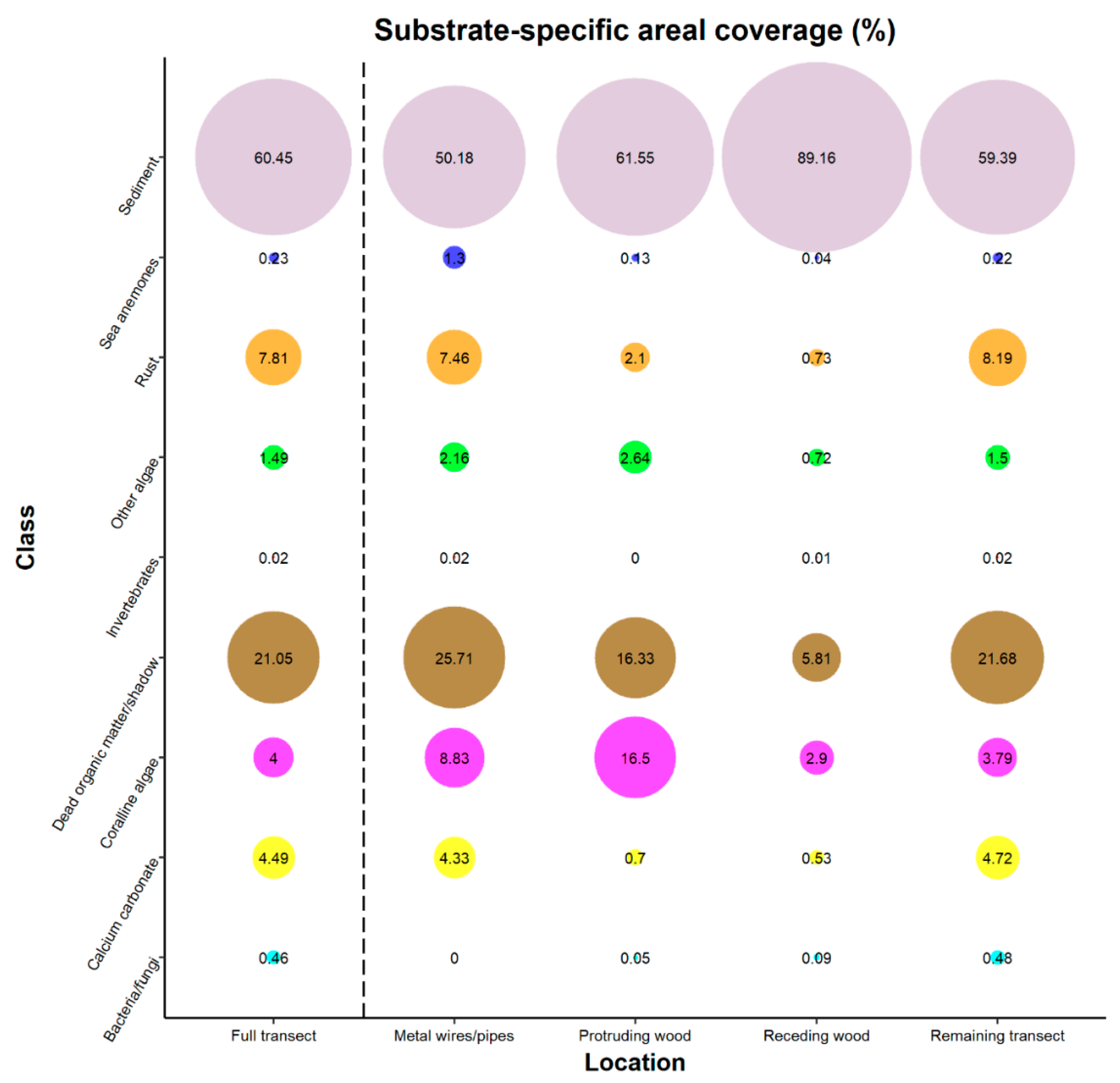
Table 3. Estimated areal coverage (number of pixels and %) of biofouling and non-biofouling spectral classes in four discrete subset areas of the underwater hyperspectral imaging (UHI) transect corresponding to metal wires/pipes, protruding wood, receding wood and the remaining transect. The table also shows the equivalent estimates for the full transect. The final two columns show the results of chi-squared (χ2) comparisons of biofouling vs. non-biofouling pixel coverage in archaeological subset areas (metal wires/pipes, protruding wood, and receding wood) vs. the remaining transect.
SubstrateCoverage of Biofouling
Spectral Classes
Coverage of Non-Biofouling Spectral ClassesChi-Squared (χ2) Comparison to Remaining Transect
Number of Pixels%Number of Pixels%χ2 Statisticp Value
Metal wires/pipes97216.64486983.36207.94<2.2 × 10−16
Protruding wood122920.01491279.99537.23<2.2 × 10⁻¹⁶
Receding wood7384.2916,44595.71728.25<2.2 × 10⁻¹⁶
Remaining transect44,55110.73370,58389.27--
Full
transect
47,49010.69396,80989.31--

