Abstract
Routine maintenance of drainage systems, including structure inspection and dredging, plays an essential role in disaster prevention and reduction. Autonomous systems have been explored to assist in pipeline inspection due to safety issues in unknown underground environments. Most of the existing systems merely rely on video records for visual examination since sensors such as a laser scanner or sonar are costly, and the data processing requires expertise. This study developed a compact platform for sewer inspection, which consisted of low-cost components such as infrared and depth cameras with a g-sensor. Except for visual inspection, the platform not only identifies internal faults and obstacles but also evaluates their geometric information, geo-locations, and the block ratio of a pipeline in an automated fashion. As the platform moving, the g-sensor reflects the pipeline flatness, while an integrated simultaneous localization and mapping (SLAM) strategy reconstructs the 3D map of the pipeline conditions simultaneously. In the light of the experimental results, the reconstructed moving trajectory achieved a relative accuracy of 0.016 m when no additional control points deployed along the inspecting path. The geometric information of observed defects accomplishes an accuracy of 0.9 cm in length and width estimation and an accuracy of 1.1% in block ratio evaluation, showing promising results for practical sewer inspection. Moreover, the labeled deficiencies directly increase the automation level of documenting irregularity and facilitate the understanding of pipeline conditions for management and maintenance.
1. Introduction
Unavoidably, global climate change brings powerful earthquakes and short-delay massive rainfall incidents. Countries worldwide are eager to invest heavily in long-term solutions to reduce the loss of life, property, environment, and economy, in which underground pipelines carrying out the transportation of drainage, sewage, and natural gas can be deemed as one of essential infrastructure. In terms of improving floods, regional drainage, and urban wastewater management, both upgrading existing drainage systems and maintaining sewer pipelines are critical components of infrastructure construction. Pipes may suffer from erosion, damage, deformation, leakage, siltation, obstruction, and other defects due to long-term deterioration. These defects may not only reduce the design efficiency of the drainage system but also cause the road surface to collapse due to the loss of foundations. When encountering heavy rain, any of each is the reason leading to flooding. As a result, a routine pipeline inspection is compulsory to provide early detection of safety hazards and preventive measures and assist in reconstructing the underground spatial distribution, avoiding construction blind spots, and accidentally digging pipelines to cause a casualty.
Currently, sewer inspection mainly relies on a manual field survey, which is difficult and tedious. Operators have to stay underground and face potential hazards due to the closed and under-ventilated environment. The on-site conditions of pipelines are recorded with images and a sketch for locations, and then assessed by technicians. However, without the help of experienced operators and detail pipeline diagrams, the pipeline conditions might be misinterpreted, and the locations of abnormal parts might be incorrect due to the limited space and inaccessibility of small pipelines. Thus, how to provide a reliable interpretation and accurate locations of pipeline defects safely still need to be addressed. To this end, specific robots were developed to replace human resources by going into underground pipelines for inspection. The systems can be classified as autonomous and cable-tethered robots according to their operating methods [1,2]. Autonomous robots typically equipped a variety of high-end sensors with a digital map to infer their geolocations. The biggest problem is the endurance of the battery power and the difficulty in arranging and removing equipment from the maintenance hole of a pipeline without a cable connection [3]. By contrast, cable-tethered robots can be retrieved by pulling back a cable, but the cable length restricts the inspection range.
On the other hand, robots can be classified into wheeled, tracked, snaking, caterpillar, and screw types according to their moving pattern. Wheeled and tracked robots usually have an excellent capability to adapt to uneven paths, while snaking and caterpillar ones are suitable for bending ways. Screw robots provide a simple structure but are slow in moving [4,5,6,7]. For missions of sewer inspection, commercial robots or platforms often embedded delicate sensors such as sonar, LiDAR, poisonous gas detector, or locator. The volume of these robots would not be suitable for small pipelines, and the maintenance cost and the equipment prices are usually high. Thus, most of the current inspecting robots mainly rely on closed-circuit television (CCTV) to collect optical images for experienced operators to examine the conditions of the pipelines, in which defects in pipes in terms of structure and functionality can be read as Table 1. It can be understood that visual-based inspection relies on sufficient lighting, which is lacked in a pipeline environment. However, providing artificial lights often leads to unbalanced illumination within the narrow pipeline, degrading the quality of visual imaging. Moreover, in the absence of quantitative data, manual visual inspection would be subjective and may lead to omission and errors. Since the global positioning system (GPS) signals are not available in underground pipelines, locations of defects are typically determined by timestamp or rough distance measurement. Indeed, in most cases, the position accuracy may conform to the requirement for region renovation. Still, the positioning reliability should be improved, considering the operation time and cost of excavation engineering is expensive.

Table 1.
Pipeline defects.
Traditional methods usually applied image edge line detection [8], image infiltration [9], and local binary mode [10] to assist in visual inspection on images of CCTV. Recently, learning-based methods such as the convolutional neural network (CNN) have achieved promising performance in object recognition and thus provide a new opportunity for abnormal identification of pipeline circumstances [11]. Various variants like region-based convolutional neural networks (R-CNN), fast R-CNN, faster R-CNN, and you only look once (YOLOv3) can be found in the literature [12,13,14]. For example, [15] used a convolutional neural network (CNN) to detect concrete cracks and compared the results with conventional edge detection approaches, namely Canny and Sobel algorithms. This study suggested that CNN revealed better detection results concerning completeness and accuracy. However, learning-based methods require satisfactory training samples, which would increase the difficulty in data collection and processing. Given the-state-of-art learning-based models in the literature, the mask region-based convolutional neural network (Mask-RCNN) [16], which uses feature pyramid networks (FPN) to solve the issue of different scale and size of training data and to search for targets through region proposal network (RPN), achieves superior performance in object recognition. In addition, the image masks of identified targets can support more information regarding target shapes or areas. Thus, Mask-RCNN was leveraged for pipeline defect recognition in this study.
In this study, a pipeline inspection platform consisted of low-cost components, such as infrared and depth cameras, as well as a g-sensor, is proposed. The inspection focuses on reporting structural and functional defects, obstacles, and flatness of a pipeline. Moreover, the moving trajectories of the platform can assist the reconstruction of a 3D pipeline map. With the help of a deep-learning approach, defects can be automatically identified along with semantic labels. The trajectory of the platform is determined by integrating image pose estimation with simultaneous localization and mapping (SLAM) techniques [17,18], improving the accuracy of positioning and the efficiency of establishing documents. Obstacles in the front are identified, and the pipeline block ratio can be estimated consequently. Moreover, signals derived from the g-sensor further reflect the flatness of a pipeline, in which abnormal pipeline regions are determined based on an adaptive threshold without manual intervention. Provided that the geolocation of the starting point in a pipe has been known, the actual moving trajectory of the platform can then be reconstructed. The proposed platform can provide not only precise geolocations but also a high level of automation and feasibility for decision support in routine sewer inspection.
2. Concepts and Methodology
This study integrated multiple sensors consisted of a Kinect depth camera, a pair of infrared cameras, a g-sensor, and raspberry pi (a small single-board computer) on a small caterpillar platform. As shown in Figure 1, the depth camera was set forward, while two infrared cameras were placed on the two sides of the platform to collect the information of lateral pipeline surfaces. The front depth camera, which consisted of three built-in sensors, acquires infrared, optical, and depth images simultaneously and generates point clouds from the depth information automatedly. The g-sensor was placed near the center of the mass to reflect the vibration of the platform. Notably, the boresight angles, lever-arm, and camera calibration have been conducted beforehand.
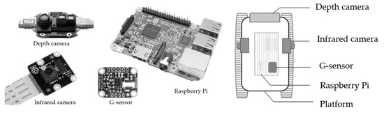
Figure 1.
Sensors and configuration used in this study.
Table 2 shows the collected data types where the depth camera can simultaneously acquire depth (512 × 424 pixels), optical (1920 × 1080 pixels), and infrared (512 × 424 pixels) images providing radiation and depth information in a scene. Typically, infrared imaging has the same limitations as any optical camera that depends on reflected light energy leading to short imaging range and poor contrast. Active infrared imaging projects a beam of near-infrared energy, so when it bounces off an object, an imager can detect the infrared energy and convert it into an electronic signal for imaging, which would be more adaptable to a pipeline environment. In this study, infrared images acquired from the lateral infrared cameras are introduced to the defect recognition of internal pipeline surfaces. In contrast, data acquired by the front depth camera are used to estimate the pipeline block ratio and identify abnormalities that obstruct the pipeline. The blocking rates and identification of the obstacles can reveal whether the pipeline demands urgent for maintenance, supporting the formulation of a management plan and increasing the automation level of documenting abnormalities. In addition, depth information rendered in the local coordinate system of depth camera can describe geometric conditions within a pipeline. To this end, point cloud SLAM is carried out to register the depth information of each timestamp and combined with infrared image pose estimation to determine the moving trajectory of the platform. Finally, the vertical accelerating variation reported by the g-sensor can show the pipeline flatness along the moving path, indicating silt conditions within a pipeline.
Table 2.
The collected data types.
Figure 2 demonstrates a hypothetical state in a pipeline when five datasets are acquired. Image data, including infrared and depth information, are obtained respectively from the three sensors at each timestamp, in which point clouds based on the local coordinate system of the depth camera can be generated simultaneously. The data capture rate and platform moving rate should associate to obtain sufficient image overlaps for subsequent analysis, which is of importance for keyframe selection. As shown in Figure 2, the three sensors are synchronized and associated with each other by prior calibration, and the black square indicates the predetermined location of the starting point. The path of the depth camera expresses the trajectory of the platform. Notably, a pipeline map is not necessary to be known in advance but the global coordinates of a starting point to determine the datum of the movement in practice. Inevitably, the absence of control points would lead to a drift of overall SLAM trajectory due to the accumulated errors among each frame. This study combined the estimates derived from the point cloud SLAM and infrared image pose estimation (image SLAM) to determine the positions of the platform at each timestamp, reducing the drift effects.
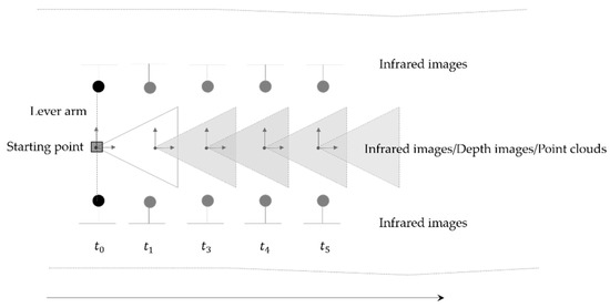
Figure 2.
Illustration of image data collection.
As inspecting platform moving, point cloud SLAM finds transformation to align newly acquired data with the current one while the platform is moving, updating the pose of the platform. Concurrently, new infrared images are respectively added to the front, left, and right image sequences to carry out image pose estimation, in which the calculations of point cloud and image SLAM are independent threads. However, the poses of the depth camera derived from point cloud SLAM are treated as initial values to define the scale factor of the image models, and the final positions of the platform are determined by examining the estimates of the three image SLAM threads, reducing the drift effect.
Figure 3 shows the block diagram of the proposed data processing, in which the input data comprises infrared and depth images as well as accelerating signals obtained during a pipeline inspection. The working scheme is composed of five sections, including obstacle identification, point cloud SLAM, image triplet pose estimation (image SLAM), internal defect identification, and flatness analysis to achieve intelligent pipeline inspection. The front depth and infrared images are applied to realize the platform positioning as well as to identify whether obstacles exist along the pipeline. If obstructions are detected, their cross-section areas can be computed to report the block ratio of the pipe. Similarly, the left and right infrared image sequences are not only applied to platform positioning but also used to identify the internal defects of the pipeline surfaces. Notably, to ease the drift effects due to the absence of control points in a pipeline, the platform trajectory is determined by taking both the pose results derived from the point cloud SLAM and the image pose estimation into account. In addition, by analyzing the acceleration signals, the flatness along the pipeline can be reflected, and the abnormal areas can be further indicated. The following sections present the details of all these processes.
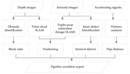
Figure 3.
The block diagram of the proposed scheme.
2.1. Positioning in a Pipeline
Practically, a node of a pipeline, which often is a manhole with a known geodetic coordinate, would be assigned as a starting point representing the initial platform position. This study exploited point cloud SLAM and image pose optimization (image SLAM) to build a cost-efficient way to realize odometry in a pipeline. Thus, the relative poses and the moving directions of the platform concerning the previous time step can be determined based on the local coordinate system sequentially. Furthermore, the geodetic location of the starting point and that of the prior manhole would be used to calculate azimuth of each position to compute the geodetic coordinates of each estimated position derived from the SLAM process. In cases, inspecting operators merely need to use the location of a manhole as a reference and measure the distances of defects for documentation. Under this circumstance, the resultant platform positions of this study are unnecessary to link to a global coordinate system. Indeed, the mid and low-end sensors adopted in this study might not provide accurate depth measurements or high image resolution, which would affect the positioning quality of the platform but remain supporting the demand for underground pipeline management.
This study leveraged the well-known Iterative Closest Point (ICP) algorithm [19] along with specific disposal to conduct the point cloud SLAM. As the platform moves and generates a point cloud, the ICP defines the optimal transformation between the new point cloud and the referenced one to determine the platform position. The computation iteratively minimizes the sum of squares of offset distances between the closest points within the two datasets. Let and be two sets of point clouds, respectively, ICP estimates the best transformation to minimize the error function:
where T is the transformation between these two sets of point clouds and indicates the error function. However, the original ICP assumes that a point set is a subset of the other. Thus, its quality and robustness are easily impaired by factors such as noise, outliers, resolution differences, and, in particular, insufficient overlapping geometry [20]. Nevertheless, ICP has attracted much attention from various communities because of the practical and straightforward idea. Numerous variants have been developed to improve the accuracy and robustness of the original ICP [21,22,23,24,25]. The configuration of ICP-based SLAM methods among extensive variants can be induced into four parts, which consisted of data refinement, matching exploration, outlier rejection, and convergence mechanism [26]. Generally, several filters are applied to eliminate singular points and noises of point clouds for data refinement. In addition, to render more geometric information, normal vectors of each point can be computed based on their K nearest neighbors [27]. Matching exploration finds presumed point pairs between two datasets by carrying out point-to-point or point-to-plane distance thresholding, in which point-to-plane distance thresholding is particularly suitable for environments that partly composed of planar structures. Moreover, the distance ratio matching [28] using the ratio of the closest and the second closest points verifies the reliability and robustness of a match. Finally, the convergence mechanism determines if the iterative calculation is convergent. In each iteration, ICP concludes a transformation consisted of rotation and translation parameters, in which the translation parameters can be used to recover the movement of the inspecting platform while the rotation parameters can describe the variation in platform orientation between in this period. In cases that the incremental parameters of rotation and translation below predetermined thresholds, the iterative process terminates. On the other hand, the iterative process is deemed as divergence if the number of iterations exceeds a given threshold.
In the aspect of infrared image pose estimation, this process combines the estimates of the point cloud SLAM with calibrated parameters to provide initial values of each frame straightforwardly. In addition, the calculation is conducted in image triplets to gain robust matches with the stable intersecting geometry of rays. Consequently, a nonlinear least-square adjustment based on three-view geometry can be formulated in a Gauss–Helmer model, which provides the basis of the incremental bundle adjustment for subsequently added images.
As shown in Figure 4, the rotation matrix and translation vector compose the relative orientation, in which the first image triplet defines the reference coordinate system whose initial values for relative orientation are given by the estimates of the point cloud SLAM. Thus, the orientation parameters can go through a nonlinear least-square adjustment for optimization. The object function describing the three-view geometry can be read as:
where and are the rotation matrix and translation vector, respectively. represents the baseline vector and represents the imaging beam of the conjugate point in each image. When three images are available, the scale-invariant feature transform (SIFT) descriptor [28] is adopted to extract image features, and a cross-search strategy [29] along with a quasi-random sample consensus (RANSAC) [30] is applied to determine corresponding point triplets in the images. In cases that the number of triple correspondences is lower than a predefined threshold, the new image is ignored, and matching proceeds for the next newly collected image.
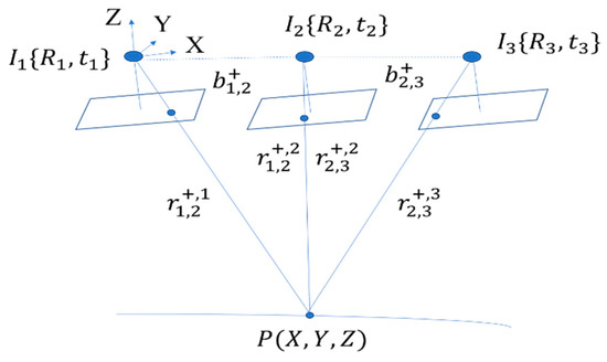
Figure 4.
The geometry of a point triplet.
Since the relative pose estimation of an image triplet with calibrated cameras has 11 degrees of freedom, the minimal required observations are four-point triplets disregarding degenerate cases, which can be formulated by the Gauss–Helmert model:
where , , , , and denote the observation vector, the error vector, the discrepancy vector, the vector of incremental unknowns, and the weight matrix, respectively; and are the partial derivative coefficient matrices concerning unknowns and observations, respectively.
Since the infrared cameras keep sensing as the inspecting platform moves, a new collected image will go through SIFT feature extraction and find corresponding point triplets with the two previous oriented images to form a new image triplet. Similarly, the pose approximations of the new image can be derived from the estimates of point cloud SLAM for subsequent refinement. The adjustment should be conducted incrementally and carried out based on sliding image triplets to work with image sequences. Therefore, the Gauss–Helmert model in Equation (3) can be reformulated into a Gauss–Markov model by rearranging as . Then, let be the new observation vector and be the new error vector. The linear model is yielded:
In the formulation of incremental least-square adjustment, the unknown vector can be divided into two components. The first portion contains the exterior orientation parameters of the images that have been included in the previous calculation, whereas the second portion indicates the exterior orientation parameters of the newly collected image whose initial values can be derived from the point cloud SLAM process. Similarly, the observation vector consists of two components and , representing the observations that have been used in the previous calculation as well as the new observations from the current image triple. Therefore, Equation (4) can be extended as [31]:
where the first row of Equation (5) indicates the adjustment based on to determine only, whereas the second row expresses the relationship between the new observation and the unknown parameters both in and in . Finally, the details of the incremental solution for the unknown parameters can be referred to [29,31]. The positions of the inspecting platform are reconstructed by integrating the resultant poses derived from both left and right infrared image sequences in the mapping coordinate system.
As illustrated in Figure 5, the reconstruction is done by applying a coordinate transformation between the depth camera frame and the two infrared camera frames, respectively. As stated above, the pose estimation of each camera is an independent thread but founded on the same coordinate system. Let the positions of the left and right infrared cameras at timestamp be expressed as , and , respectively. The left infrared camera frame is related to the depth camera frame by a rigidly defined lever arm and boresight matrix while the right infrared camera frame is associated with the depth camera frame by and . Similarly, the front infrared camera frame is related to the depth camera frame by a rigidly defined lever arm and boresight matrix . Thus, the positions based on the depth camera frame can be read as:
where , indicates the depth, front, left, or right cameras. Consequently, the , , and are weighted to determine the position of the platform at timestamp as:
where describes the positions of the platform at timestamp. , , and indicate the posterior standard deviation of unit weight of each pose estimation, respectively.
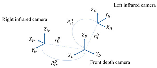
Figure 5.
The geometry of a point triplet.
2.2. Internal Defect Identification
Regarding the pipeline defects listed in Table 1, this study focused on detecting the cracks of inner pipeline surfaces as well as the obstacles along the pipeline and further examining the geometric attributes of the anomalies. The internal defect identification is applied to the images acquired from the front and lateral infrared cameras by leveraging learning-based image recognition techniques. Deep learning approaches for image recognition have been widely explored in recent years, which provide a revival of the classic artificial-intelligence method of neural networks, e.g., [32,33,34,35,36]. Among the state-of-the-art approaches such as the YOLO or faster R-CNN that integrates feature extraction, region proposal, classification, and bounding-box regression into a unified, the Mask-RCNN model with a feature pyramid network backbone was leveraged in this study. Additionally, a transfer learning strategy [37] was performed referring to the pre-trained weights of the Microsoft COCO [38] for specific labels of cracks. The applied model was trained on the common defects consisted of over five labeled instances in 1000 images to identify pipeline abnormality. With the help of image bounding boxes and masks, the locations and shapes of the identified anomalies can be revealed. For a crack instance, the principal and second axes of its masks can be defined by the principal component analysis (PCA). Therefore, as shown in Figure 6, the length of this crack can be determined via the extreme points along the principal axis and estimated by using the conception of ground sample distance (GSD). Similarly, the maximum and minimum width of the crack can be observed along the second axis, providing geometric information about the identified cracks.
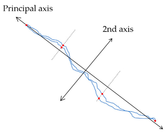
Figure 6.
The principal component analysis (PCA) principal and second axes of a crack.
On the other hand, the infrared images covering the front conditions are applied to identify anomalies that obstruct a pipeline based on the same Mask R-CNN module. If a defect is detected and identified, its sectional area is estimated by using the conception of GSD. The average depth of the obstacle mask defines the object distance from the platform, therefore the GSD can then be computed by the proportional relations depicted in Figure 7.
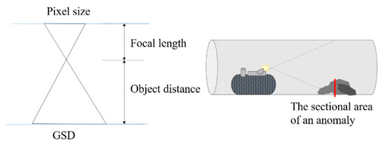
Figure 7.
The estimation of the sectional area.
In addition, the area in object space covered by a pixel is defined as the square of GSD. Consequently, the sectional area of the obstacle can be roughly estimated by counting the pixel number within the mask. Thus, a blockage ratio that takes the sectional area of an obstacle to be divided by that of a pipeline can be computed as:
where represents the blockage ratio; and indicate the sectional areas of an obstacle and a pipeline, respectively. The rate would reflect the situation of obstruction in a pipeline, supporting the decision for pipeline management.
2.3. Flatness and Slope Analysis of a Pipeline
The inspecting platform reflects the flatness of a pipeline by analyzing the vertical acceleration behavior obtained from the embedded g-sensor revealing the effects of functional defects of a pipe such as sediments, ponding, or scum.
If the platform goes through an anomaly, the g-sensor will occur apparent vertical acceleration variation, as depicted in Figure 8. Most of the existing methods exam these conspicuous signals with a predefined threshold to determine abnormal areas along the path. However, how to provide a reliable threshold adaptably is still needed to be addressed. This study applied an adaptable thresholding method to detect abnormal vibration, reflecting the flatness in a pipeline referring to [39]. To this end, this study took 1 Hz as a unit to compute the standard deviation of the vertical acceleration signals in this epoch. The average of the standard deviation of all current units is calculated, and thus the discrepancy of each unit towards all current units in amplitude can be read as [39]:
where indicates the standard deviation of the i-th unit; represents the mean of all current is a constant describing the amplitude multiple of the i-th unit relative to the whole current units. The range of is ranged from 0 to 3, expressing the relative roughness level, and the expression is applied to the vertical acceleration of each unit to determine whether abnormal signals occur. If the of a unit is more significant than 1, the unit is categorized into an abnormal one. The judgment can be read as:
where represents the group of abnormal units. The magnitude of each unit will be updated when an itinerary is finished. Consequently, the irregular sections in a pipeline can be determined obviating the need for manual setting a predefined threshold.
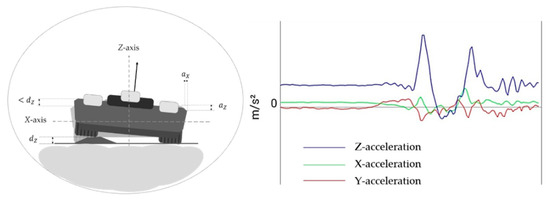
Figure 8.
The demonstration of the acceleration behavior.
3. Validation and Analysis
As illustrated in Figure 9, a controllable environment that simulated a section of a box culvert was used to evaluate the proposed indoor positioning and the internal defect identification methods. Figure 9 shows the floor plan of the testing field, in which the straight distance between the starting and ending points is 5.40 m. A local coordinate system originated at the starting point was established by using theodolite equipment, and the coordinates of the centers of three obstacles, a bump, seven checkpoints, and the endpoint were set along the path accordingly.
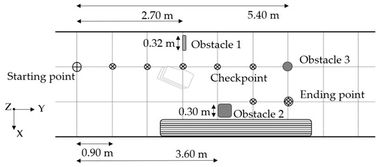
Figure 9.
The floor plan of the testing field.
Regarding the configuration of the platform, a Kinect depth camera was set forward, while two infrared cameras were placed facing the left and right sides of the platform, respectively. The three sensors had been synchronized, and the data collection rate was about 16 Hz. The timestamps of keyframes were selected regarding the overlapping ratios derived from left and right image sequences, respectively. In this case, the inspecting platform patrolled from the starting point to the ending point in a one-direction enclosed path. Table 3 shows a fraction of the collected data comprising infrared images in three directions as well as depth image and point clouds that are inputs for the proposed method.
Table 3.
A faction of the collected data.
Figure 10a illustrates the result of the point cloud SLAM. In contrast, Figure 10b uses red color lines to depict the poses of the moving platform at eight timestamps along with the actual path in yellow color, in which a slight drift occurred as the platform moving forward. The overall registration quality reported by the interior accuracy of ICP was 0.028 m. However, the root-mean-square error (RMSE) of the registration derived from checkpoints showed a deviation of 0.067 m. Subsequently, the platform poses were introduced to the estimation of infrared image orientation as initial values for further refinement.
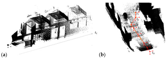
Figure 10.
The on-site point cloud (a), and the estimated (red) and actual (yellow) moving trajectories (b).
The left part of Figure 11 depicts the refined positions of the platform in the point cloud with the same timestamps. On the other hand, the right part of Figure 11 shows the refined coordinates in which the distance parallel to the Z-axis is about 5.43 m revealing a deviation of 3 cm regarding the actual value, namely a relative accuracy of 0.005 m.

Figure 11.
The refined positions derived from the image simultaneous localization and mapping (SLAM).
On the other hand, Figure 12 highlights the discrepancy in the checkpoint accuracy of the image and point cloud SLAM, in which the checkpoints are set along the moving trajectory and ordered by the distance from the origin, as illustrated in Figure 9. In light of Figure 12, the drift effects do turn conspicuous while the moving length of the platform increases. The point cloud SLAM revealed an RMSE of 0.093 m in platform positioning. In contrast, the proposed SLAM reflected an RMSE of 0.064 m recovering a more accurate moving trajectory, in which the most significant positioning error is about 0.09 m, namely a relative accuracy of 0.016 m.
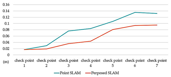
Figure 12.
The positioning deviation resulted from image and point cloud SLAM.
Table 4 demonstrates partial results of the defect identification, in which the obstacles in the heading direction are not only detected but also their sectional areas are estimated. In addition, the internal defects are identified in the left infrared images whose length, width, and area are evaluated, respectively. The distance of each obstacle profile is computed by the average depth information of its identified mask so that the relevant GSD can roughly estimate the sectional area. On the other hand, the lateral distances are determined regarding the platform positions in the point cloud. The internal defects such as cracks and flaking are identified, as shown in Table 4, where the length and the width of the crack are about 75 cm and 15 mm, respectively. The areas of the flaking regions are about 347 and 1949 , respectively. In addition, the flatness analysis based on acceleration signals does reflect the bump set along the path, showing its feasibility. Details on the acceleration analysis can be referred to [30] for more discussion.
Table 4.
The results of the internal defect identification.
Nevertheless, by manual checking, the values of the geometric information seem overestimated around ±0.9 cm in this case, especially in the width of the cracks. Still, the area estimates of flaking regions and the obstacles in the front can approach the actual values. The obstacles in the forward direction are all detected and identified correctly. However, the loss rate of the internal defects is about 5% since the capability of the low-end sensor restricts the effectiveness of the recognition process.
For further assessment, a tube with a small diameter, as shown in Figure 13, is used to have an insight into the estimation of the block ratio in a pipeline, and tiny cracks are applied to the defect identification. In this case, a stone with the known size is placed with different poses to simulate obstacles in the pipeline, and the internal defect identification is then conducted to detect the barriers and estimate the block ratio, reflecting the pipeline condition.
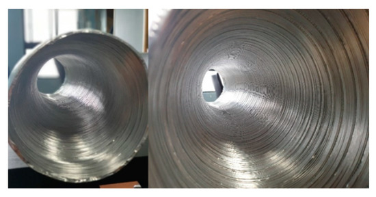
Figure 13.
The tube with a small diameter.
Figure 14a–d illustrate the four identified obstacles with a correct stone label of stone no matter the difference in object distances. Table 5 indicates the quantitative results of the evaluation, in which the block ratios reveal a deviation of around ±1.1% compared to the manual assessment, reporting the faithful status of the pipeline and highlighting the effectiveness of the proposed method.
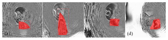
Figure 14.
The visual results of the identified obstacles.
Table 5.
The evaluated results of the internal defect identification.
Moreover, to gain insight into the effectiveness of the defect identification for tiny crack detection, an assessment of the completeness and the length estimation is carried out and then verified with those derived from the manual measurement. Figure 15a–d depict the four results of tiny crack detection, while Table 6 shows the quantitative indices regarding the detecting completeness of cracks.
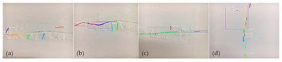
Figure 15.
The four results of tiny crack detection.
Table 6.
The quantitative indices of the crack detection.
In the light of Figure 15 and Table 6, cracks (a) and (b) express the same break but reveal a noticeable difference of 25.9% in the detection rates. It implies that the repeatability of the Mask-RCNN model in detecting tiny cracks is unstable, leading to inadequate completeness. The loss rate of crack detection is about 40%. Nevertheless, once the amount and multiplicity of the training samples are increased, the effectiveness should be improved.
4. Discussions
Compared to those studies that conduct SLAM only based on point clouds or image graphs [18,27,40], the main difference of this study is the optimization of the platform positioning. Most studies find the poses of a platform by minimizing the positional error of points matched between two consecutive datasets. These processes usually lead to a vast linearized system to be solved at every iteration. By contrast, this study integrated point cloud and three-way images to conduct the SLAM process. As rigorous pose estimation of image sequences demands initial values for a nonlinear solution, estimates result from point cloud SLAM can be used to define the scale of image models and treated as approximations to converge rapidly and prevent resulting in local minima. In addition, by leveraging the learning-based image recognition technique, the proposed system can not only identify internal pipeline defects but also recognize obstacles in the heading direction. The geometric attributes of these targets and the block ratio of a pipeline can be further computed to aware of pipeline conditions for management and maintenance. Additionally, the unstable performance of a low-cost g-sensor affects the performance of reflecting the pipeline flatness. Different devices may lead to variant evaluation results. Therefore, the proposed system leveraged an adaptable thresholding method to analyze the acquired acceleration signals. The determination results can be more consistent regardless of the performance of a g-sensor device.
Indeed, the current experimental condition was certainly ideal compared to real sewer environments. This study focused on the validation of the proposed method and evaluated the effectiveness and feasibility of this phase, considering the policy restrictions and safety of the crew. Typically, the real conditions of a poor-performance sewer pipeline are often in a mess. The inspecting platform may confront numerous functional defects, such as deposition, obstacles, roots, ponding, and scum, resulting in a lot of noise in the collected image or point cloud data. Similarly, if sewer environment conditions are mostly symmetric and repetitive patterns or low textures, inevitably, disqualified pose estimation and a high loss rate of object recognition would occur. Nevertheless, the proposed system can be deemed as an alternative to assist manual sewer inspection cost-effectively and more securely.
5. Conclusions
This study presented an intelligent pipeline inspection platform consisted of low-cost components. The experiment results validate the effectiveness of the proposed positioning strategy and internal defect identification. By integrating the pose estimates derived from the point cloud SLAM and three-way image SLAM, the reconstructed moving trajectory of the platform can mitigate the drift effects achieving a relative accuracy of 0.016 m when no additional control points deployed along the inspecting path. In addition, the geometric information of observed defects accomplishes an accuracy of 0.9 cm in length and width estimation and an accuracy of 1.1% in block ratio evaluation. The inspecting platform not only provides visualization of the identified entities and expresses geometric information such as block ratio of a pipeline and the sizes of crack defects but also capable of indicating the geolocations of identified incidents. The identified deficiencies can be labeled directly increasing the automation level of documenting irregularity and facilitate the understanding of pipeline conditions for management and maintenance.
To increase the working flexibility and feasibility, future improvements following the proposed method will explore other auxiliary sensors such as inertial measurement unit (IMU) to facilitate initial pose estimation. IMU data would support the computation stability, even the point cloud and image data are contaminated by noise due to unfavorable on-site conditions. Moreover, the proposed will tend to increase the amount and the multiplicity of the training samples regarding pipeline defects or explore other radial bands to improve the effectiveness of the defect identification process. Last but not least, this study will seek collaboration with the authority to conduct an actual field survey in the future.
Author Contributions
T.-Y.C. provided the research conception and design and analysis of the experiments and revised and finalized the manuscript. C.-C.S. contributed to drafting the manuscript and the implementation of proposed algorithms. All authors have read and agreed to the published version of the manuscript.
Funding
This research received no external funding.
Acknowledgments
This publication would not be possible without constructive suggestions from reviewers, which are much appreciated.
Conflicts of Interest
The authors declare no conflict of interest.
References
- Nassiraei, A.A.F.; Kawamura, Y.; Ahrary, A.; Mikuriya, Y.; Ishii, K. Concept and Design of A Fully Autonomous Sewer Pipe Inspection Mobile Robot “KANTARO”. In Proceedings of the 2007 IEEE International Conference on Robotics and Automation, Roma, Italy, 10–14 April 2007; pp. 136–143. [Google Scholar] [CrossRef]
- Kim, J.-H.; Sharma, G.; Iyengar, S.S. FAMPER: A Fully Autonomous Mobile Robot for Pipeline Exploration. In Proceedings of the 2010 IEEE International Conference on Industrial Technology, Vina del Mar, Chile, 14–17 March 2010; pp. 517–523. [Google Scholar] [CrossRef]
- Knedlová, J.; Bílek, O.; Sámek, D.; Chalupa, P. Design and Construction of an Inspection Robot for the Sewage Pipes. MATEC Web Conf. 2017, 121, 01006. [Google Scholar] [CrossRef]
- Imajo, N.; Takada, Y.; Kashinoki, M. Development and Evaluation of Compact Robot Imitating a Hermit Crab for Inspecting the Outer Surface of Pipes. J. Robot. 2015, 6, 1–7. [Google Scholar] [CrossRef] [PubMed]
- R&R VISUAL, INC. (800) 776-5653. Available online: http://seepipe.com/ (accessed on 31 January 2020).
- Roh, S.; Choi, H.R. Differential-Drive in-Pipe Robot for Moving inside Urban Gas Pipelines. IEEE Trans. Robot. 2005, 21, 1–17. [Google Scholar]
- Kwon, Y.-S.; Yi, B.-J. Design and Motion Planning of a Two-Module Collaborative Indoor Pipeline Inspection Robot. IEEE Trans. Robot. 2012, 28, 681–696. [Google Scholar] [CrossRef]
- Jahanshahi, M.R.; Masri, S.F. Adaptive Vision-Based Crack Detection Using 3D Scene Reconstruction for Condition Assessment of Structures. Autom. Constr. 2012, 22, 567–576. [Google Scholar] [CrossRef]
- Yamaguchi, T.; Hashimoto, S. Fast Crack Detection Method for Large-Size Concrete Surface Images Using Percolation-Based Image Processing. Mach. Vis. Appl. 2010, 21, 797–809. [Google Scholar] [CrossRef]
- Hu, Y.; Zhao, C. A Novel LBP Based Methods for Pavement Crack Detection. JPRR 2010, 5, 140–147. [Google Scholar] [CrossRef]
- Szegedy, C.; Liu, W.; Jia, Y.; Sermanet, P.; Reed, S.; Anguelov, D.; Erhan, D.; Vanhoucke, V.; Rabinovich, A. Going Deeper with Convolutions. In Proceedings of the 2015 IEEE Conference on Computer Vision and Pattern Recognition (CVPR), Boston, MA, USA, 7–12 June 2015; pp. 1–9. [Google Scholar] [CrossRef]
- Redmon, J.; Farhadi, A. YOLOv3: An Incremental Improvement. arXiv 2018, arXiv:1804.02767. [Google Scholar]
- Girshick, R.; Donahue, J.; Darrell, T.; Malik, J. Rich Feature Hierarchies for Accurate Object Detection and Semantic Segmentation. In Proceedings of the 2014 IEEE Conference on Computer Vision and Pattern Recognition, Columbus, OH, USA, 23–28 June 2014; pp. 580–587. [Google Scholar] [CrossRef]
- Girshick, R. Fast R-CNN. In Proceedings of the 2015 IEEE International Conference on Computer Vision (ICCV), Santiago, Chile, 7–13 December 2015; pp. 1440–1448. [Google Scholar] [CrossRef]
- Cha, Y.-J.; Choi, W.; Büyüköztürk, O. Deep Learning-Based Crack Damage Detection Using Convolutional Neural Networks. Comput.-Aided Civ. Infrastruct. Eng. 2017, 32, 361–378. [Google Scholar] [CrossRef]
- He, K.; Gkioxari, G.; Dollár, P.; Girshick, R. Mask R-CNN. In Proceedings of the 2017 IEEE International Conference on Computer Vision (ICCV), Venice, Italy, 22–29 October 2017; pp. 2980–2988. [Google Scholar] [CrossRef]
- Grisetti, G.; Kümmerle, R.; Stachniss, C.; Burgard, W. A Tutorial on Graph-Based SLAM. IEEE Intell. Transp. Syst. Mag. 2010, 2, 31–43. [Google Scholar] [CrossRef]
- Borrmann, D.; Elseberg, J.; Lingemann, K.; Nüchter, A.; Hertzberg, J. Globally Consistent 3D Mapping with Scan Matching. Robot. Auton. Syst. 2008, 56, 130–142. [Google Scholar] [CrossRef]
- Besl, P.J.; McKay, N.D. A Method for Registration of 3-D Shapes. IEEE Trans. Pattern Anal. Mach. Intell. 1992, 14, 239–256. [Google Scholar] [CrossRef]
- Fusiello, A.; Castellani, U.; Ronchetti, L.; Murino, V. Model Acquisition by Registration of Multiple Acoustic Range Views. In Computer Vision—ECCV 2002; Heyden, A., Sparr, G., Nielsen, M., Johansen, P., Eds.; Lecture Notes in Computer Science; Springer: Berlin/Heidelberg, Germany, 2002; pp. 805–819. [Google Scholar] [CrossRef]
- Bae, K.-H.; Lichti, D.D. A Method for Automated Registration of Unorganised Point Clouds. Isprs J. Photogramm. Remote Sens. 2008, 63, 36–54. [Google Scholar] [CrossRef]
- Habib, A.; Bang, K.I.; Kersting, A.P.; Chow, J. Alternative Methodologies for LiDAR System Calibration. Remote Sens. 2010, 2, 874–907. [Google Scholar] [CrossRef]
- Al-Durgham, M.; Habib, A. A Framework for the Registration and Segmentation of Heterogeneous Lidar Data. Available online: https://www.ingentaconnect.com/content/asprs/pers/2013/00000079/00000002/art00001 (accessed on 10 March 2020).
- Gruen, A.; Akca, D. Least Squares 3D Surface and Curve Matching. ISPRS J. Photogramm. Remote Sens. 2005, 59, 151–174. [Google Scholar] [CrossRef]
- Akca, D. Co-Registration of Surfaces by 3D Least Squares Matching. Available online: https://www.ingentaconnect.com/content/asprs/pers/2010/00000076/00000003/art00006 (accessed on 10 March 2020).
- Pomerleau, F.; Colas, F.; Siegwart, R. A Review of Point Cloud Registration Algorithms for Mobile Robotics. Found. Trends Robot. 2015, 4, 1–104. [Google Scholar] [CrossRef]
- Mendes, E.; Koch, P.; Lacroix, S. ICP-Based Pose-Graph SLAM. In Proceedings of the 2016 IEEE International Symposium on Safety, Security, and Rescue Robotics (SSRR), Lausanne, Switzerland, 23–27 October 2016. [Google Scholar]
- Lowe, D.G. Object Recognition from Local Scale-Invariant Features. In Proceedings of the Seventh IEEE International Conference on Computer Vision, Kerkyra, Greece, 20–27 September 1999; Volume 2, pp. 1150–1157. [Google Scholar] [CrossRef]
- Reich, M.; Unger, J.; Rottensteiner, F.; Heipke, C. On-Line Compatible Orientation of a Micro-Uav Based on Image Triplets. ISPRS Ann. Photogramm. Remote Sens. Spat. Inf. Sci. 2013, 3, 37–42. [Google Scholar] [CrossRef]
- Stamatopoulos, C.; Chuang, T.Y.; Fraser, C.S.; Lu, Y.Y. Fully Automated Image Orientation in the Absence of Targets. In International Archives of the Photogrammetry, Remote Sensing and Spatial Information Sciences; XXII ISPRS Congress: Melbourne, Australia, 2012; Volume 39B5, pp. 303–308. [Google Scholar] [CrossRef]
- Beder, C.; Steffen, R. Incremental Estimation without Specifying A-Priori Covariance Matrices for the Novel Parameters. In Proceedings of the 2008 IEEE Computer Society Conference on Computer Vision and Pattern Recognition Workshops, Anchorage, AK, USA, 23–28 June 2008; pp. 1–6. [Google Scholar] [CrossRef]
- Parekh, H.S.; Thakore, D.G.; Jaliya, U.K. A Survey on Object Detection and Tracking Methods. Int. J. Innov. Res. Comput. Commun. Eng. 2014, 2, 2970–2979. [Google Scholar]
- Long, Y.; Gong, Y.; Xiao, Z.; Liu, Q. Accurate Object Localization in Remote Sensing Images Based on Convolutional Neural Networks. IEEE Trans. Geosci. Remote Sens. 2017, 55, 2486–2498. [Google Scholar] [CrossRef]
- Jiao, J.; Zhang, Y.; Sun, H.; Yang, X.; Gao, X.; Hong, W.; Fu, K.; Sun, X. A Densely Connected End-to-End Neural Network for Multiscale and Multiscene SAR Ship Detection. IEEE Access 2018, 6, 20881–20892. [Google Scholar] [CrossRef]
- Leibe, B.; Schindler, K.; Cornelis, N.; Van Gool, L. Coupled Object Detection and Tracking from Static Cameras and Moving Vehicles. IEEE Trans. Pattern Anal. Mach. Intell. 2008, 30, 1683–1698. [Google Scholar] [CrossRef]
- Akcay, S.; Kundegorski, M.E.; Willcocks, C.G.; Breckon, T.P. Using Deep Convolutional Neural Network Architectures for Object Classification and Detection Within X-Ray Baggage Security Imagery. IEEE Trans. Inf. Forensics Secur. 2018, 13, 2203–2215. [Google Scholar] [CrossRef]
- Pan, S.J.; Yang, Q. A Survey on Transfer Learning. IEEE Trans. Knowl. Data Eng. 2010, 22, 1345–1359. [Google Scholar] [CrossRef]
- Lin, T.-Y.; Maire, M.; Belongie, S.; Hays, J.; Perona, P.; Ramanan, D.; Dollár, P.; Zitnick, C.L. Microsoft COCO: Common Objects in Context. In Computer Vision—ECCV 2014; Fleet, D., Pajdla, T., Schiele, B., Tuytelaars, T., Eds.; Lecture Notes in Computer Science; Springer International Publishing: Cham, Switzerland, 2014; pp. 740–755. [Google Scholar] [CrossRef]
- Chuang, T.-Y.; Perng, N.-H.; Han, J.-Y. Pavement Performance Monitoring and Anomaly Recognition Based on Crowdsourcing Spatiotemporal Data. Autom. Constr. 2019, 106, 102882. [Google Scholar] [CrossRef]
- Lu, F.; Milios, E. Globally Consistent Range Scan Alignment for Environment Mapping. Auton. Robot. 1997, 4, 333–349. [Google Scholar] [CrossRef]


© 2020 by the authors. Licensee MDPI, Basel, Switzerland. This article is an open access article distributed under the terms and conditions of the Creative Commons Attribution (CC BY) license (http://creativecommons.org/licenses/by/4.0/).