1. Introduction
The new generation of orbital Synthetic Aperture Radar (SAR) platforms can deliver several types of all-weather products. It can be used to observe and analyze several aspects of the land cover, which is often done in conjunction with information obtained by optical sensors. It is common, however, that SAR data is the only choice available for specific tasks, such as land cover classification in areas constantly covered by clouds. Therefore, it is important to develop methods suitable to extract the most from SAR data, when no other option is available.
Nonetheless, the main issue with radar data usage and processing is the multiplicative nature of the speckle noise, typical for this type of sensor, and its relatively low discriminative power when compared with optical data in many applications. Consequently, real classification problems with radar data are generally limited to four or fewer classes [
1,
2].
A way of trying to overcome these difficulties is to use
Region-Based Classification (RBC), also referred to as
Geographical Object-Based Image Analysis (GEOBIA) [
3]. RBC methods first aggregate pixels into homogeneous objects, or regions, using a segmentation procedure. Then a classifier, exploiting spectral, textural, and/or morphological features, assigns a class to each region/segment. The segmentation step, however, relies on image data only and ignores semantics, which generally leads to suboptimal image partitioning [
3].
Moreover, segmentation is known to be an ill-conditioned problem because it admits multiple solutions, and a small change in the input image may lead to significant changes in the segmentation outcome. Indeed, it is generally difficult to model a visual perception strategy for detecting regions, which justify the large number of segmentation algorithms proposed over the years [
4]. Additionally, most segmentation algorithms proposed thus far were designed for optical images, and few techniques designed for radar data are available [
5].
Common to all segmentation algorithms is the existence of a number of parameters, whose values are often determined empirically, via a trial-and-error process. Tuning the segmentation parameter values for a particular application and input images is, therefore, usually a complex, multi-objective task, which can be time demanding [
6]. Considering also the different scales and spectral characteristics of objects from the different classes of interest, one can argue that it may be impossible to find a particular set of segmentation parameter values that are optimum for all the different object classes, and that tuning segmentation for each individual class would be more appropriate. The main problem with this approach would be that, in the general case, conflicting subdivisions of the image, that is, segments posteriorly assigned to different classes may overlap spatially, and such conflicts should be resolved at a later stage in the classification process.
The task that usually follows the segmentation step is to classify the detected regions and assign each one to a class. The most common region classifiers are based on statistical distances [
7,
8], which are normally developed using the Gaussian assumption. The classification problems evaluated in this work consider a number of generalized classes at a time, representing, thus, a multi-modal classification problem, which makes the Gaussian assumption less suitable.
Considering the problems mentioned above, some scientific issues are especially relevant:
Is it possible to develop a methodology, for land-use/land-cover classification (LULC) using solely SAR data, capable of delivering acceptable results when considering four or more classes?
Are the proposed RBC approaches introduced in this work (in
Section 2.1.2) better than a standard RBC approach (e.g.,
Section 2.1.1) for the classification of SAR data?
Would it be better to optimize segmentation parameter values considering all classes, or each class individually (as discussed in
Section 2.1.1 and
Section 2.1.2)?
Can automatic class-wise optimization of segmentation parameters (by a procedure such as the one described in
Section 2.2.3) provide good results for RBC on SAR data?
How to obtain an overall RBC map when doing per-class segmentation and classification?
In this context, this paper proposes and evaluates novel approaches for SAR data classification, which rely on specialized segmentations, and on the combination of partial maps produced by classification ensembles. Such approaches comprise a meta-methodology, in the sense that they define a systematic set of operations, which can be carried out by virtually any segmentation and classification algorithm, and optimization procedure.
The following general hypotheses have been considered in the development of the meta-methodology:
Using a smaller number of classes, which is the opposite of specialization, will favor the generalization capacity of a given classifier, which will improve the classification accuracy measured on independent/unseen data.
Specializing segmentation for each individual class of the classification problem provides for a better delineation of objects from different classes, which will, in turn, favor the global classification process.
Two case studies were conducted to validate the proposed approaches. One example used a single channel X-band airborne image, and a complete reference map produced through visual interpretation. Another example used an L-band Palsar image obtained over the Tapajos National Forest, Brazil, with references collected in-situ. Although, as said before, the proposed approaches are independent for their main components, in this work we use a particular set of methods for the implementation of those components, namely:
A method called
MultiSeg [
8], which was designed to segment radar data, exploiting its particular statistical properties.
An optimization tool called
Segmentation Parameters Tuner (SPT) [
6] to automatically select a set of optimal segmentation parameter values based on reference objects.
A recently proposed method for region classification, based on support vector machines (SVM) [
7], is considered more robust for the classification of radar data without any source of ancillary data.
This paper is organized as follows.
Section 1 presents the proposed meta-methodology.
Section 2 describes the particular choice of methods used in the validation experiments.
Section 3 describes the study areas, materials, and the experimental setup. In
Section 4 we present and discuss the results of the experiments. Finally, we present conclusions and directions for further work.
2. Materials and Methods
In this work, we evaluated two novel region-based approaches, employed in the classification of SAR images, namely Class-Specific Segmentation with Single-Class Classification (CSS-SCC) and Class-Specific Segmentation with Multi-Class Classification (CSS-MCC). Both approaches rely on segmentations tuned (or specialized) for each class considered in a particular classification problem. In the following sections, we describe such approaches in terms of meta-methodologies, in the sense that potentially any particular techniques for segmentation, parameter tuning, and classification could be selected.
We compare the classification performances of the proposed approaches with those delivered by another region-based approach, denoted Multi-Class Segmentation and Classification (MSC), which represents the basic processing chain of region-based image classification. Moreover, we evaluate two variants of the MSC approach. The first one relies on segmentations tuned automatically for all classes (collectively). In the second variant, denoted ad hoc Multi-Class Segmentation and Classification (MSCAH), we use default segmentation parameter values.
We further compare all the above-mentioned region-based approaches with two baseline pixel-based methods, relying respectively on Maximum Likelihood (ML) classification, and on Support Vector Machines (SVMs). ML is one of the most popular supervised classification methods in Remote Sensing (RS) [
9]. Following the Bayes theorem, the ML classifier assigns a pixel to the class with the highest likelihood, considering the respective probability density functions derived from the training data. SVMs have also been extensively used in the classification of RS data [
10]. An SVM aims to fit an optimal separating hyperplane between classes by focusing on samples that lie at the edge of the class distributions, the support vectors. SVMs can efficiently perform non-linear classification by using kernel functions that map their inputs into higher dimension feature spaces. Several types of kernels have been proposed, including sigmoidal, polynomial, and Radial Basis Function (RBF). In this work, the pixel-based baseline SVM classifier uses an RBF kernel.
2.1. Region-Based Classification Approaches
In the next sections, we further describe the region-based classification approaches evaluated in this work. In the following, denotes the set of c classes of interest.
2.1.1. Multi-Class Segmentation and Classification (MSC)
In the Multi-Class Segmentation and Classification (MSC) approach, image segmentation is first carried out to delimit homogeneous regions, according to particular homogeneity criteria. Next, features (or properties) of the segments are computed and used in the subsequent classification step, which assigns class labels to the different segments.
In the MSC approach, all segments later subjected to classification are generated using a particular segmentation algorithm and a single set of segmentation parameter values. The goal of the segmentation procedure is, therefore, to delineate as well as possible all objects of all classes considered in the classification problem.
In the experiments, we consider two variants of the approach. In the first variant (referred to in the sections that follow simply as MSC), the segmentation parameter values are tuned automatically, considering objects of all classes. In this case, parameter tuning is carried out with the optimization procedure described in
Section 3, which takes as inputs a few manually delineated reference segments of all classes of interest.
In the second variant, the ad hoc Multi-Class Segmentation and Classification (MSCAH), the parameter values of the segmentation procedure are not tuned, as the respective default (arbitrary) values are used.
2.1.2. Class-Specific Segmentation (CSS)
An alternative to MSC is to carry out independent segmentations for each individual class of interest, a strategy called hereinafter Class-Specific Segmentation (CSS).
CSS involves performing a specific segmentation for each class, thus making it possible to optimize the parameter values of the segmentation algorithm for each individual class considered in the classification problem. In fact, in this strategy, different segmentation algorithms could be selected for different classes. The parameter values are also determined according to the procedure described in
Section 3, but contrary to the MSC strategy, the set of manually delineated reference segments used as input of the optimization procedure contains references of a single target object class.
Once the optimal segmentation parameter values for a particular class of object are found, an (independent) segmentation is performed. As specialized segmentations are carried out for each class, the CSS strategy introduces an important issue to the classification process, i.e., segments associated with different classes will eventually overlap. There is, therefore, the need to perform some sort of spatial conflict resolution at the end of the classification process.
2.1.3. Class-Specific Segmentation with Single-Class Classification (CSS-SCC)
In this work, we propose and evaluate two alternative classification strategies for the segments generated using CSS. The first alternative has to do with performing a binary classification over the outcome of each class-specific segmentation. We call this approach Class-Specific Segmentation with Single-Class Classification (CSS-SCC).
In CSS-SCC, after a class-specific segmentation, the generated segments are subjected to a classifier, which classifies those segments as belonging to a particular class ωi or to a class that corresponds to the merging of all other classes except ωi (denoted as ῶi), in a procedure denoted Single-Class Classification (SCC).
In the training stage, the accuracy of each single-class classification is computed (based on validation data), to establish a rank of classes, in which the highest-ranked class is the one associated with the most accurate classification, and the lowest-ranked class is associated with the worst classification.
After a single-class classification is performed, say for class ωi, the segments classified as belonging to the “other classes,” ῶi, are discarded. At this point it is important to notice that all segments belonging to the same class will be disjoined by construction, but segments belonging to different classes may overlap each other.
To solve the eventual spatial conflicts among segments associated to different classes, a topological overlay procedure is carried out: if two segments overlap each other, the segments associated with the lower-ranked class will be clipped, losing the intersection area. Note that during this procedure, some classified segments may completely disappear. At the end of the overlay procedure, the remaining segments may keep their original shapes, have their areas reduced or even be divided into two or more segments.
In the event that a particular region of the scene is assigned to no class, i.e., the respective extent was classified as “other classes” in all single-class classifications, the region is assigned to the class with the maximum a priori probability.
Figure 1 shows a graph with the processing chain of the CSS-SCC approach.
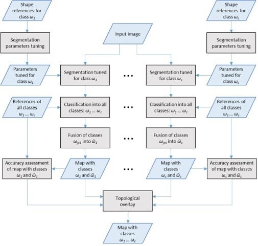
2.1.4. Class-Specific Segmentation with Multi-Class Classification (CSS-MCC)
Yet another classification strategy for the segments generated using CSS was evaluated in this work. We call this strategy Class-Specific Segmentation with Multi-Class Classification (CSS-MCC).
In CSS-MCC, the classification strategy differs from the one used in CSS-SCC as the classification of each class-specific segmentation considers all classes. That is, the classifiers involved are trained to classify the segments produced by each class-specific segmentation into any of the classes considered in the classification problem, in what is denoted as Multi-Class Classification (MCC). In this stage, a set of c classifications is already available for consideration and accuracy analysis.
Furthermore, after the multiclass classification of a segmentation tuned for class
ωi, the segments classified as belonging to the other classes,
ωj≠i, are assigned to a class
ῶi, which represents the fusion of all
ωj≠i classes. From this point on the procedure is similar to what was described for CSS-SCC, as shown in
Figure 2.
2.2. Methods
Although the classification approaches described in the previous section represent meta-methodologies in the sense that potentially any specific technique can be adopted for segmentation, parameter tuning, and classification, we briefly describe in this section the techniques that were actually employed in the experiments carried out to validate the proposed approaches.
2.2.1. Region-Based Classification with SVM
As mentioned before, the use of only spectral data, as in the case of pixel classification, may be unsatisfactory in some cases, for example, in the presence of noise or when the data has high spatial and spectral resolutions. An alternative to mitigate this problem is the
Region-Based Classification (RBC). In this approach, the pixels are initially aggregated into homogeneous objects by an image segmentation procedure and then individually classified [
11].
Let be an image defined on a support , is a set of disjoint image regions or segments , is the feature space, and denotes the feature vector of region , whereby . In simple terms, represents the segments generated by a segmentation procedure, segments cannot overlap each other, and each segment is associated with a set of features, or properties, , such as average intensity values of the pixels that belong to the segment, standard deviation of such intensity values, and so on.
A classifier may be represented by a function , which assigns the feature vectors/elements of to a class in , where . That is, the classifier will classify a segment based on its property values.
The training set for class is given by , whereby indicates that segment belongs to class In other words, the classes of the segments that are used to train the classifier are known.
Many RBC classifiers [
11] have been proposed. As the focus of this research is not a comparison among different versions of RBCs, just one was chosen, based on SVM because of its known qualities.
The main objective of the SVM consists of finding a binary separating hyperplane between training samples, with the largest possible margin. The separating hyperplane is the geometric location where the following linear function is equal to zero:
where
w represents the orthogonal vector to the hyperplane,
is the distance from the hyperplane to the origin, and
denotes the inner product. Therefore, the SVM classifier tries to find the regions in the feature space associated with the different classes. For a thorough discussion about SVM and its training procedure, [
12] is suggested.
Equation (1) represents a separation hyperplane defined in the original feature space of the data. Mapping the input data from the original to another space is a strategy to improve the accuracy of SVM. Such mapping and classification into a new space can be performed using a kernel function, which replaces the inner product in (1) and in the equations related to the training of SVM.
Particularly, [
7] proposed the following kernel function to deal with the observation distribution (PDF) within regions as a single input:
where
is the Battacharyya distance between multivariate Gaussian models corresponding to regions
and
, each one belonging to each class in the training set. The Bhattacharyya distance measures the similarity of two probability distributions. Equation (2) shows, therefore, that by using such kernel function, a segment will not be classified taking into consideration aggregated (single) features values, but rather, the distribution of features values associated with all pixels that belong to a segment. This particular kernel has the additional useful characteristic of not needing any particular estimation of kernel parameters like the RBF, which requires the estimation of the kernel spread. Details about it can be found in [
12]. The SVM used for the baseline pixel-based classification, however, uses the RBF kernel, as referred in the beginning of
Section 2.
Additionally,
is a large enough constant added to make
be a metric. It is supposed that support vectors found during the training phase would match the prevailing modes in the reference data. In the experiments reported in
Section 4, the region-based classifications were carried out with SVMs using the kernel function shown in Equation 2.
2.2.2. Segmentation with MultiSeg
MultiSeg consists of a specialized segmentation technique for SAR and optical imagery [
8]. This section presents an overview of the MultiSeg processing chain. Initially, the input image is resampled at different rates creating an image pyramid of various compression levels. Then a region growing procedure is performed at the highest compression level. In sequence, a split and merge-based technique is applied to the intermediate levels in turn, from the coarser to the finer level, all the way down to the original image scale.
The region growing procedure initially considers each pixel at a particular level as a segment. As segments are visited in a random order, the procedure evaluates if the current segment can be merged to its most similar neighbor, being the measure of similarity the module of the difference between the segments’ mean intensity pixel values. A segment is only merged to its mutual best neighbor, that is, the best neighbor of the current segment’s best neighbor must be the current segment. The condition for a merge to occur is that the means of the sets of pixel values within the region candidates are considered statistically indifferent—above a user-defined confidence level— according to a t-Student hypothesis test. The region growing procedure stops when no more merges are possible.
Processing starts at the next level below with the refinement of the borders of each segment defined at the previous level. The refinement process visits all pixels that intercept the segment border and decides if each of such pixels should be kept in the segment or be assigned to a neighboring segment. The decision is based on a test that considers the distance from the current pixel value to the mean value of the neighboring segments, weighted by their variances, which in the case of SAR data takes into consideration the equivalent number of looks of the current compression level.
After the border refinement step, a homogeneity value for each segment is computed. The measure of homogeneity takes into consideration the coefficient of variation of the segment’s pixel values. A segment is considered heterogeneous if its homogeneity measure is below a critical value threshold, which is defined considering the different statistical properties of SAR and optical data. In short, homogeneity critical values for SAR data are defined based on the assumption of a Gamma distribution of pixel values and considering different numbers of equivalent looks, segment sizes, and confidence values.
Segments considered heterogeneous are then subjected to the region growing procedure described above. After all heterogeneous segments have been processed, the whole collection of segments in that compression level is also subjected to the region growing procedure. Again, the region growing stops when no merges are possible. Processing resumes recursively at the next finer compression levels until the original image level is reached. After that level is processed, all segments smaller than a user-defined area threshold are merged to their most similar neighbor. MultiSeg’s complete processing chain is depicted in
Figure 3.
The algorithm described above for a single band image can be generalized in MultiSeg for multiple bands (multispectral optical data or multiple polarized SAR data) [
8].
2.2.3. Segmentation Parameter Values Tuning with SPT
A key issue regarding image segmentation is the selection of its parameter values, which depends on the target application. This selection can be done manually, by a trial-and-error process, or in an automatic fashion. Manual tuning of these parameters is time-consuming and without any guarantee to lead to the optimal set of values due to the dependency on subjective human perception. On the other hand, automatic methods are proposed to minimize human intervention either in unsupervised or supervised fashions.
Unsupervised methods [
13] rely on statistical measures without considering semantics [
14,
15]. On the other hand, supervised methods, e.g., [
16,
17], consider semantics by manually delineating segment samples, which symbolize a “good segmentation” for the user.
Optimization algorithms are employed to search the parameter space for the set of values that provide a segmentation outcome that best matches the user-provided samples. This match is quantified by an empirical discrepancy metric.
There are many works [
14,
15,
16] proposing different ways to tune parameters for the multiresolution segmentation algorithm (MRG) [
17]. None of these works, however, are evaluated with SAR images.
In this context, Segmentation Parameter Tuner (SPT) [
6] offers an automatic way to tune parameters for MultiSeg [
8], a hierarchical segmentation algorithm for either optical or SAR data, using a set of single-solution, population-based, or hybrid metaheuristics.
Let’s define
as the set of parameter values of a segmentation algorithm. Then, the optimal set of values, hereafter denoted as
, is defined as
where
measures the discrepancy between the outcome of the segmentation algorithm,
, running with parameter values
and a set of Reference Segments,
, which represents the expected outcome. Equation (3) shows, therefore, that the parameter values obtained with the optimization procedure carried out with SPT are the ones that produce the segments similar to those in the reference segment set.
Figure 4 summarizes SPT’s processing steps.
First, the input image is segmented with an initial set of parameter values (randomly generated between a given range defined by the user). Then, the metric value is computed using the segmentation outcome and the references. These steps are repeated with the new set of parameter values generated by the metaheuristic till a stopping criterion is reached (e.g., a maximum number of iterations).
SPT offers a number of metaheuristics, such as Differential Evolution, Generalized Pattern Search, Mesh Adaptive Direct Search, and Nelder-Mead [
6]. In this work, we selected Differential Evolution (DE), which is briefly explained in the following paragraph.
DE belongs to the family of evolutionary strategies. The optimization process works iteratively through generations of a group of individuals specified by their corresponding genes. In our case, each gene corresponds to a segmentation parameter value (
). An individual is a set of genes that represents a putative solution (
). A set of individuals forms a population, which evolves in a number of generations. At each generation, the fitness (metric’s value) of each individual is evaluated. In the following generations, the less suited individuals are discarded and new individuals are generated from the best ones through the so-called genetic operators of mutation and crossover, which retain the values of some variables of the best individuals and modify other variables based on heuristics. The process goes on until a stopping criterion is met, typically a given number of generations [
18].
In this work, we selected the
Precision and Recall metric, which delivers a measure
F [
19] that takes values in the interval [0, 1], whereby
F equals 1 when the segmentation outcome perfectly matches the reference.
2.3. Experimental Analysis
In this section, we present the study areas and the specific techniques used for segmentation, parameter tuning, and classification.
2.3.1. Study Areas
In the experiments, we selected two areas covered by SAR images with different characteristics, acquired by different sensors, one aboard an airplane, the other aboard an orbital platform.
The study areas are located in the northern region of Brazil, inside the Amazon basin. The first area, hereinafter denoted Paragominas, is a rural area in the municipality of Paragominas, located in the southeast of the state of Pará. The second area, hereafter called Tapajós, is a forested area within the Tapajós National Forest, in the west of Pará state. Both regions are frequently covered by clouds, which makes it very difficult to be imaged by optical sensors.
Paragominas
The Paragominas image was acquired in February 2007 with the airborne interferometric synthetic aperture radar ORBISAR-1 [
20]. The image, an X-band, single-channel (HH), has a spatial size of 2.5 m × 2.5 m and covers an area of approximately 12.91 km
2. The area is covered essentially by mature forest, regeneration fields, pasture, and bare soil, so those were the four classes considered in the classification problem, and for which reference patches were determined by a photo interpreter acquainted with the area. In
Figure 5, we show the Paragominas image and the reference patches, used for training the classifiers, and for accuracy evaluation.
Table 1 shows the number of classified patches used for training and evaluation, and their respective sizes in terms of the number of pixels.
Tapajós
The Tapajós image was acquired on 29 June 2010, with the Phase Array L-Band Synthetic Aperture Radar (PALSAR) sensor, aboard the Advanced Land Observing System (ALOS). The image is L-band, dual-channel (HH and HV), has a pixel spacing of 12.5 m × 12.5 m, and covers an area of approximately 185 km2. The area is covered by six classes: mature forest, regeneration in advanced and intermediate stages, pasture, agricultural crops, and bare soil; which were considered in the classification problem. Reference patches of each of the classes were determined by a photo interpreter acquainted with the area.
In
Figure 6, we show the Tapajós image (HH polarization) and the reference patches, used for training the classifiers and for accuracy evaluation. A colored composition (bands 5,4,3) of a Landsat 7 image of the study area, acquired on 29 June 2010 (
Figure 5c) is also shown for a visual reference.
Table 2 shows the number of classified patches used for training and evaluation, and their respective sizes in terms of the number of pixels.
2.3.2. Classification Setup
For each study site, a number of training points (pixels) from the training patches (see
Figure 5 and
Figure 6) were randomly selected to train all the classifiers used in this work. A total of 2000 pixels were selected for each class in the Paragominas site, and 400 pixels for each class in the Tapajós site.
In addition to the previously described MSC, CSS-SCC, and CSS-MCC approaches, a pixel-based Maximum Likelihood (ML) classifier, and an SVM, with a Radial Basis Function kernel, were also trained and evaluated to serve as baselines.
In the case of the CSS-SCC and CSS-MCC approaches, the accuracies of the intermediate (individual) classification were measured using 1000 and 300 randomly selected pixels for the Paragominas and Tapajós sites respectively. Note that the pixels selected for such accuracy assessment were not contained in the set of pixels used for training the classifiers. The accuracy metric selected for all cases was the global Kappa value [
21].
2.3.3. Segmentation Setup
As mentioned before, the procedure for the selection of optimum parameter values for the segmentation procedure in the MSC, CSS-SCC, and CSS-MCC approaches was carried out with SPT, using the Differential Evolution (DE) metaheuristic.
DE was set up with a population of 20 individuals, running for 4 generations. Additionally, the discrepancy metric (fitness function) used was Precision and Recall. The parameters of MultiSeg that had their values optimized in the process were number of compression levels, similarity threshold, confidence level, and minimum area. In each experiment, DE was run three times with the above-mentioned configuration, but with a different, randomly generated initial population.
In the next section, we also show the results of experiments for which the segmentation parameter values were not optimized, and the proposed, default values of MultiSeg were used. As mentioned before, we denote this approach ad hoc Multiclass Segmentation and Classification (MSCAH). In all such experiments, the parameter values were the number of compression levels equal to 5; similarity threshold equal to 1; confidence level equal to 0.95; minimum area equal to 20 pixels.
2.3.4. Accuracy Assessment
For each study site, a number of testing points from the test patches (see
Figure 5 and
Figure 6) were randomly selected to assess the classification accuracies of the different classification schemes investigated. A total of 1000 points were selected for each class in the Paragominas site, and 300 points for each class in the Tapajós site. In the following section, accuracies are given in terms of users’ accuracies and Kappa values.
The user’s accuracy indicates the probability that prediction represents reality. It is calculated by dividing the correctly classified pixels in a class by the total number of pixels that were classified as belonging to that class.
The Kappa coefficient [
21] reflects the difference between the agreement of the classification results with the reference data and the agreement expected by chance alone. For example, a Kappa value of 0.75 means there the classifier provides a 75% better agreement than what would be obtained by chance alone.
3. Results and Discussion
In the following sections, we present and discuss the results obtained for the various classification schemes, in each study site.
3.1. Results on Paragominas Dataset
Table 3 and
Table 4 summarizes the accuracy of all classification schemes evaluated in this paper.
Table 4 shows specifically the results of the CSS-MCC approach, with segmentations optimized for the different classes of interest.
As
Table 3 shows, the pixel-based classification methods [
22] delivered the worst results. In these cases, the single SAR channel classification is comparable to a simple thresholding operation, which is very sensitive to noise. In both cases, the accuracies obtained were unsatisfactory.
Although still low, and somewhat comparable to the pixel-based methods, the accuracy improvement observed for the MSCAH approach, shows that the classification benefitted from the RBC strategy, even without tuning segmentation parameters, as a result of the noise reduction brought by the segmentation process.
The accuracy improvement noticed for the MSC approach can, however, be considered a significant one, a 35% improvement with respect to the Kappa value obtained with the best pixel-based method (SVM). Anyhow, the Kappa value obtained (0.61) can still be considered to be low.
A substantial increase in classification accuracy was brought by the CSS-SCC (class-specific segmentation—single class classification) approach, which presented a Kappa value approximately 20% higher than that of the MSC approach, in which a single segmentation, optimized considering all the classes of interest, was performed. This result indicates that optimizing the segmentation for the individual classes can, indeed, be beneficial.
Another explanation for the accuracy improvement brought by the CSS-SCC approach is that it breaks down a complex, multimodal classification problem into simpler problems, in a way that is similar to an ensemble of classifiers. In this approach, the task of each classifier in the ensemble is basically to discriminate between a particular class and all other classes of interest, and the best classifiers in the ensemble have priority in eventual classification conflicts.
Table 3 also shows that the performance of CSS-MCC was approximately 10% lower than that of the CSS-SCC approach. This result indicates that the increase in complexity brought by the fact that the classifiers in the ensemble needed to discriminate all four classes of interest, while the CSS-SCC classifiers needed only to distinguish a single class from the background (all other classes), actually hinders overall classification. The superiority of the CSS-SCC approach in this case also seems to indicate that the ensemble with simpler classifiers can show a higher generalization capacity than an ensemble with more complex classifiers.
Table 4 shows the accuracies related to the individual classifications obtained prior to the final overlay procedure in the CSS-MCC approach.
The second to fifth columns are associated with segmentations tuned to classes listed in the row, whereas the sixth column represents the UA obtained after the overlay procedure (same values as in the CSS_MCC column in
Table 3). The third to sixth rows refer to the class the UA was computed on, and the last two rows contain the Kappa values and the Overall accuracy. It can be observed that the classification of the segmentation optimized for the soil class reached an overall Kappa value of 0.77, an expressive result, especially when compared with the pixel-based and MSCAH approaches. As pointed out in
Section 2.2.2 the CSS-MCC can present intermediate results, in this case with four classes that can already be considered for choice. In another circumstance, if, for example, the class Forest is of the sole interest of an application, the segmentation tuned for Regeneration, which delivers a user accuracy of 97% for Forest.
3.2. Results on Tapajós Dataset
Table 5 and
Table 6 summarize the accuracy of all classification schemes evaluated in this paper.
Table 6 shows specifically the results of the CSS-MCC approach, with segmentations optimized for the different classes of interest.
Like what was observed in the experiments of the Paragominas site,
Table 5 shows that the pixel-based classification methods [
22] delivered the worst results. Both classifiers delivered a map with a Kappa coefficient of approximately 0.35. Moreover, the lower Kappa values in comparison to those obtained in the Paragominas experiments seem to corroborate the notion that standard radar data does not provide for acceptable accuracy for a classification problem with a larger number of classes.
The superior accuracy observed for the MSCAH in relation to the best pixel-based method (ML) –0.52 against 0.35 Kappa value shows that the region-based approach significantly improves classification performance, even when the parameters of the segmentation procedure are not tuned, which is evidence that contextual information is fundamental in the case of relying solely on SAR data (amplitude) information.
Optimizing the segmentation parameters for objects of all classes jointly (MSC), further improved the classification accuracy to a Kappa of 0.59. Additionally, similar to what was observed in the Paragominas experiments, the best classification performance was obtained by tuning segmentation for individual classes and relying on an ensemble of binary, class-specific classifiers (CSS-SCC): 0.63 Kappa value.
In the Tapajós experiments, the final result of the CSS-MCC approach was also inferior to CSS-SCC. This time however it was also slightly inferior to MSC. We observe here that the classification problem for this site considers six classes of interest, and is, therefore, substantially more complex than the previous one.
The results of the Paragominas experiments, and the superiority of CSS-SCC in relation to MSC in the Tapajós site, indicate that tuning segmentation for the individual classes has the potential to improve overall classification accuracy. This potential was, however, not enough to compensate for the increase in classification complexity. We note that in this case the MCC ensemble had not only more complex classifiers but also a larger number of them.
Table 6 shows the accuracies of the individual classifications obtained prior to the overlay procedure in the CSS-MCC approach.
The second to seventh columns are associated with class-specific segmentation, tuned for the corresponding classes, listed in the second row, whereas the eighth column represents the UA obtained after the overlay procedure (same values as in the CSS-MCC column in
Table 5). The third to eighth rows refer to the class UA was computed on, and the last two rows contain the Kappa values and the Overall accuracy.
In this case, the classification of the segmentation optimized for the class Crop obtained the highest Kappa value: 0.66. Inspecting
Table 6, one can choose the case which delivers the best User Accuracy for a class of someone´s particular interest.
Finally, it is important to emphasize that although a Kappa value in the order of 0.63 can be deemed low in the context of optical RS image classification, it can be considered a good result in view of the difficulty of classifying more than four classes using only one channel SAR, and no ancillary data.
4. Conclusions
In this work, we propose and investigate region-based classification approaches that can boost the performance of SAR classification, particularly the cases where the only remote sensing data available is non-polarimetric SAR data. These are known as difficult cases, which are the focus of this study. The proposed approaches comprise a meta-methodology, since they are independent of the particular design and implementation of their main components, i.e., the segmentation and classification algorithms, and the segmentation parameters’ optimization procedure.
An important aspect of the proposed classification approaches is that they rely on automatically tuning the chosen segmentation algorithm’s parameter values for the particular classes of the classification problem. It is worth mentioning the use of a segmentor specialized on radar statistics, which is available for free download, and a specialized version of SVM developed for RBC.
Considering the region-based classification (RBC) framework, the results of the experiments carried out in this work indicated that the optimization of segmentation parameter values can significantly improve classification accuracy (
Table 3 and
Table 5, MSCAH and successive ones). The results also indicated that specializing segmentation for the different classes of interest was also beneficial, (CSS,
Section 2.1.2;
Table 3 and
Table 5, last two columns) as opposed to performing a single segmentation, optimized for all classes jointly (MSCAH and MSC).
Moreover, the results showed that breaking up the classification process into an ensemble of binary classifiers (CSS-SCC) was also beneficial, indicating that such a strategy can better deal with a multimodal classification problem, especially considering input features with a low discriminative capacity, as SAR amplitude values.
Table 4 (and similarly
Table 6) showed that intermediate results, on the path to CSS-MCC, can show even better accuracy than the result of CSS-MCC overlay. The conclusion is that every RBC result, with all classes of interest, in this methodology, is worth consideration.
We can conclude that segmentation optimization is an important ally for improving the results of the RBC classification of SAR images, especially the case where just one channel is available. Breaking the global classification problem into simpler, local ones have the potential to boost classification accuracy for that kind of data.
As future research, we plan to evaluate the proposed meta-methodology with different input data, particularly verifying other hard to classify source cases, such as C band radar data. Besides the important improvement in accuracy, the highest obtained Kappa value of 0.77, maybe can be still improved extracting other traditional features, like texture or shape features.
Another hard problem worth investigating is the classification of very similar classes with respect to their spectral signatures, such as classifying different, very green crops. Additionally, we plan to test and compare different segmentation and classification algorithms, and parameter optimization procedures.


 ,
, 


