Abstract
To improve the poor accuracy of the MODIS (Moderate Resolution Imaging Spectroradiometer) daily fractional snow cover product over the complex terrain of the Tibetan Plateau (RMSE = 0.30), unmanned aerial vehicle and machine learning technologies are employed to map the fractional snow cover based on MODIS over this terrain. Three machine learning models, including random forest, support vector machine, and back-propagation artificial neural network models, are trained and compared in this study. The results indicate that compared with the MODIS daily fractional snow cover product, the introduction of a highly accurate snow map acquired by unmanned aerial vehicles as a reference into machine learning models can significantly improve the MODIS fractional snow cover mapping accuracy. The random forest model shows the best accuracy among the three machine learning models, with an RMSE (root-mean-square error) of 0.23, especially over forestland and shrubland, with RMSEs of 0.13 and 0.18, respectively. Although the accuracy of the support vector machine and back-propagation artificial neural network models are worse over forestland and shrubland, their average errors are still better than that of MOD10A1. Different fractional snow cover gradients also affect the accuracy of the machine learning algorithms. Nevertheless, the random forest model remains stable in different fractional snow cover gradients and is, therefore, the best machine learning algorithm for MODIS fractional snow cover mapping in Tibetan Plateau areas with complex terrain and severely fragmented snow cover.
1. Introduction
Snow is an important water resource, and snowmelt water constitutes the main source for many rivers in mountainous areas, especially in arid regions [1]. The high albedo and low thermal conductivity of snow cover strongly affect the global radiant energy balance [2,3]. Known as the “Third Pole”, the average elevation of the Tibetan Plateau (TP) exceeds 4000 m.a.s.l. Snow in the TP is the main water source for many major rivers in Asia, including the Yellow, Yangtze, Mekong, Salween, and Ganges Rivers. Previous studies have shown that the snow thickness in the TP can significantly affect the Indian Ocean summer monsoon and precipitation [4,5] and even affect the frequency of Eurasian heat waves [6]. Seasonal snow cover is the main factor that controls the phenology and growth of alpine grassland in the TP [7,8]. In addition, excessive snowfall results in the death of many livestock and great economic losses, making it one of the major natural disasters in the TP [9].
Due to terrain ruggedness and hostile conditions, it is very difficult to monitor snow cover using manual field-based techniques; thus, remote sensing technology has become the most effective method to monitor snow cover in the TP. However, due to the impacts from strong solar radiation, snow melts quickly, and wind-blown snow can lead to serious fragmentation in the snow distribution throughout the TP area where the terrain is complex, which introduces considerable difficulties and uncertainties for the use of remote sensing data to monitor snow cover [10,11]. Moreover, traditional binary snow cover mapping using optical remote sensing data based on the normalized difference snow index (NDSI) has difficulty meeting the accuracy requirements for hydroecological and climate models [12]. Although microwave remote sensing has the advantage of being insensitive to clouds and weather conditions, the fatal drawback is its low spatial resolution, usually tens of kilometers. The coarse resolution causes great uncertainty in the TP because of the complex topography and the fragmented snow cover distribution [11]. As a result of its superior spatial and spectral resolutions, optical remote sensing has become the preferred source of data for the large-scale real-time monitoring of snow cover. The binary snow product created with the NDSI is common and popular for many optical sensors [13]. However, it is challenging for the binary snow mapping algorithm to satisfy the accuracy requirements for snow cover mapping because of the serious problem of mixed pixels in the TP [14].
The currently available remote sensing snow cover datasets include the low-resolution Climate Data Record of Northern Hemisphere Snow Cover Extent (NHSCE) and the long-term Northern Hemisphere daily five-kilometer snow cover extent product (JASMES) datasets, the medium-resolution GlobSnow, IMS (Interactive Multisensor Snow and Ice-mapping System), and MODIS datasets and the high-resolution Landsat-7/8 and Sentinel-2A datasets [13,15,16,17,18]. Recently, wet snow-covered area maps based on Sentinel-1 data have become increasingly available [19]. Taking the MODIS daily binary snow cover product (MOD10A1) as an example, the overall accuracy of this product under clear-sky conditions in Europe, the United States and northern Xinjiang of China reached 94% [20,21], but the accuracy was less than 80% in the TP [22]. Similarly, the overall accuracy of the IMS daily snow products in China exceeds 88%, but this product encounters serious omission errors in the TP. The main reason for this problem is that the IMS is unable to effectively identify mixed pixels caused by severe snow fragmentation; thus, the snow classification accuracy reaches only 45% [23]. Therefore, to improve the accuracy of snow cover mapping over the TP, the use of a fractional snow cover (FSC) mapping algorithm has become an efficient way to improve the accuracy of snow cover products.
Previous studies have shown that the linear regression algorithm employed by MOD10A1 exhibits large errors in the TP, and linear spectral mixture analysis can somehow improve the accuracy of FSC algorithms, but its accuracy is still unsatisfactory because complex terrain causes mixed pixel problems over the TP. Compared with the snow map retrieved from Landsat, the root mean square error (RMSE) of the MOD10A1 FSC is approximately 0.30, and the difference in the average FSC is approximately 6.71% in the TP [24,25]. However, machine learning algorithms boast a higher FSC mapping efficiency and accuracy than other algorithms in the TP, and the RMSE can be reduced to 0.22 [25]. Other studies have also shown that using various machine learning models can effectively improve the accuracy of FSC mapping [26,27]. In addition, unmanned aerial vehicles (UAVs) equipped with small digital cameras play an important role in scientific research because of their high data quality, low cost and small size. At present, UAV technology has enabled breakthroughs in crop yield estimation, crop-assisted breeding, disaster data collection, grassland biomass monitoring and snow cover estimation [25,28]. Nevertheless, the MODIS global FSC mapping algorithm is derived from the linear relationship of the NDSI determined by Landsat. On the one hand, the high spatial resolution of Landsat imagery can obtain relatively accurate FSC information; however, classification errors still exist, especially in mountainous and forested areas with complex topography [29]. On the other hand, the relationship between the NDSI and FSC differs due to the heterogeneity of snow cover in different regions, which constitutes the main reason for the varying accuracy of MOD10A1 among different regions. Therefore, obtaining real FSC information observed on the ground forms the basis of the MODIS FSC mapping algorithm and represents the main approach to improve the accuracy of snow cover monitoring. Moreover, the extremely high spatial resolution of UAVs can provide observations close to the ground, thereby providing reliable input parameters for the FSC mapping algorithm.
In the context of global warming, there is an urgent need for a real-time and accurate snow cover monitoring algorithm for the TP. Therefore, this study employs three machine learning algorithms based on UAV and MODIS data to improve the accuracy of the MODIS FSC product over the TP. The goals of this study are threefold: (1) to introduce true FSC values obtained by UAVs into the MODIS FSC inversion model for the TP, which is characterized by complex terrain; (2) to compare the efficiency of various machine learning algorithms in the FSC inversion process; (3) to develop an optimal FSC inversion model that can produce a more accurate FSC product based on MODIS data in the TP.
2. Study Area
The TP (26.00°N–52.77°N, 73.30°E–105.77°E) is located in Southwest China and exhibits an average elevation exceeding 4000 m.a.s.l. The total area of the TP is approximately 2.5 million km2, 41.5% of which is covered by snow in winter [10]. The topography is complex, the elevation ranges from 100 to 8848 m across the plateau, and the land cover types include mainly grassland, forestland, shrubland, bare land and cropland (Figure 1). One of the most important resources offered by the TP is its water resources, which are stored mainly in the form of glaciers and snow. Meltwater is an important source of several major rivers in China and neighboring Asian countries [30,31].
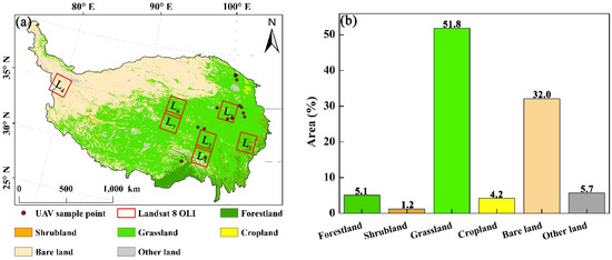
Figure 1.
(a) UAV sampling points with the footprint of the Landsat 8 OLI images used in this study and the land cover types (MCD12Q1) [32], and (b) proportions in the Tibetan Plateau (TP).
3. Data and Methodology
3.1. Data
3.1.1. UAVs
During a field survey from February 2017 to March 2018, 24 images were captured across the TP by using a Dajiang Inspire 1 Pro equipped with a GoPro Hero 3+ camera (Figure 1a). The coverage of each image was controlled to 750 × 750 m, and then 500 × 500 m images were clipped to correspond to MODIS pixels. Each image was composed of approximately 200 photos, in which the adjacent photos had an overlap of over 60%. Figure 2 shows four images as examples over different land cover types. Reference FSC data were then produced based on these UAV images to train the FSC machine learning models.
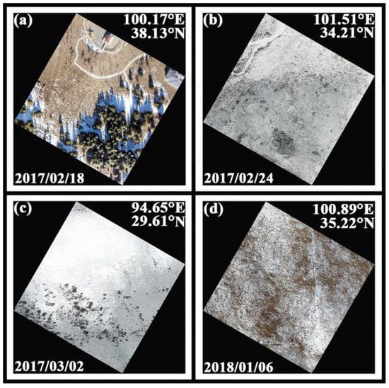
Figure 2.
UAV-captured true color composed images under the (a) forestland, (b) grassland, (c) shrubland and (d) bare land in Tibetan Plateau. Each image covers a range of 500 × 500 m.
3.1.2. Landsat
For this study, seven Landsat 8 Operational Land Imager (OLI) images acquired under nearly clear-sky conditions were collected from the United States Geological Survey website (http://www.usgs.gov/) (Figure 1a, Table 1). These images contain all land cover types across the TP, and each land cover type has at least 10,000 OLI pixels.

Table 1.
Information on the Landsat 8 OLI images.
3.1.3. MODIS
For this study, the MODIS daily snow cover product (MOD10A1 V006), surface spectral reflectance product (MOD09GA) and vegetation index product (MOD13A1) were utilized, and the data from these products correspond to the same dates as the UAV and Landsat data (http://www.nasa.gov). The MOD10A1 V006 product, which is an improved version of V005, includes four main data layers: the NDSI_Snow_Cover, NDSI, albedo and data quality assessment layers. In this study, cloudy pixels and meaningless pixels were eliminated. The FSC calculation formula for MOD10A1 (MOD) is as follows [33]:
3.1.4. Auxiliary Data
The Shuttle Radar Topography Mission digital elevation model (SRTM-DEM) with a spatial resolution of 90 m was used in this study (http://www.usgs.gov). The DEM was resampled to a resolution of 500 m and used as the input elevation data to train the machine learning model. MCD12Q1 is an annual land cover type product (https://lpdaac.usgs.gov/products/mcd12q1v006/) with a spatial resolution of 500 m [32]. In this study, to reduce complexity and improve efficiency, the MCD12Q1 land cover types in our study area during 2017 in the International Geosphere-Biosphere Programme (IGPB) classification scheme were reclassified into six categories, namely, grassland, forestland, shrubland, bare land, cropland and other lands.
3.2. Landsat Snow Cover Mapping Algorithm
The SNOWMAP algorithm was used to generate a Landsat 8 OLI binary snow map, and the normalized difference forest snow index (NDFSI) and normalized difference vegetation index (NDVI) were employed during binary snow mapping to improve the detection of snow in forested areas [29]. The snow map was then aggregated to the FSC product with a spatial resolution of 500 m.
3.3. Machine Learning
Three popular machine learning algorithms in snow cover mapping, including the random forest (RF), support vector machine (SVM) and back-propagation artificial neural network (BP-ANN) algorithms, were used to train the FSC inversion model in our study area. The BP-ANN algorithm is a commonly used machine learning algorithm that is composed of an input layer, a hidden layer and an output layer [34,35]. In this study, the parameters labeled error.criterium, Stao and method were set to “LMS”, “NA” and “ADAPTgdwm”, respectively. The number of neurons in the input layer and the number of neurons in the hidden layer are the two most important parameters of a neural network model. However, an excessive number of neurons will lead to overfitting or unnecessary operation of the model, which will lead to a low modeling efficiency [27,36]. In this study, 240 BP-ANN models were constructed on the basis of a previous empirical model [25], where the numbers of neurons in the input and hidden layers were 6 and 48, respectively, which resulted in the optimal BP-ANN model for this study.
The RF model is a nonlinear algorithm that employs a series of decision trees to achieve sufficient prediction accuracy. The theoretical basis of this model is the classification tree algorithm [37]. The bootstrap sampling method is used; accordingly, the final prediction result is selected from multiple decision trees by voting. The higher the degree of repetition is, the better the effect of the RF model.
The SVM model is a supervised learning algorithm that is often used in data analysis and pattern recognition [38]. The classification and regression processes in an SVM compose its core algorithm and are based on a group of hyperplanes constructed in high-dimensional space. The main difficulty in constructing an SVM model is setting the gamma and cost parameters; in this study, the gamma and cost parameters were debugged and determined by using the tune.svm function. The kernel function is another important parameter; in this study, the Gaussian kernel function was used.
3.4. Validation
For all three models described above, the 10-fold cross-validation method was utilized to adjust the model structure [39]. The FSC distribution retrieved from the UAV was used as the output layer and the corresponding factors, namely, the NDSI, R1, R2, R3, R4, R5 and DEM, were utilized as the input layer and were randomly divided into 10 parts for cross-validation. In the RF model, the SVM model and the BP-ANN model, one dataset was randomly selected at each moment as the test set, and the remaining 9 datasets were used as the training set; a total of 10 iterations were performed. The goodness of fit (R2), RMSE and bias were used to evaluate the fitting ability of each model, and the mean value of 10 iterations was selected. After adjusting the model structure, FSC model mapping and verification were carried out. The average accuracy (ACC), RMSE, positive average error (PAE), negative average error (NAE) and average error (AE) were adopted to evaluate the FSC models [25]. The formulas are as follows:
In the above formulas, yi represents the real FSC, yi’ represents the simulated value, i represents a specific sample, n represents the number of samples and m and r represent the numbers of pixels for which the simulated value is larger and smaller than the real FSC, respectively.
4. Result
4.1. Parameter Sensitivity Test
Figure 3 shows the snow maps retrieved from the UAV based on supervised classification. The FSC was calculated and used as the ground truth to train the three machine learning models. Before a model is trained, however, the input parameters should be screened [25]. The method employed to screen the parameters was univariate regression, which was applied between the ground truth and each parameter, and the significance of each parameter was tested by R2 and Pearson’s correlation coefficient. The test results are shown in Table 2. As a result, the surface reflectance in R1, R2, R3, R4 and R5, the NDSI and altitude were ultimately selected as the modeling parameters through the comprehensive consideration of R2 and Pearson’s correlation coefficients.
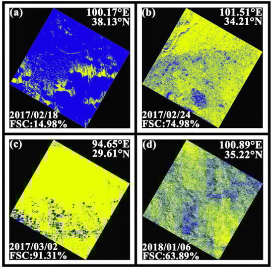
Figure 3.
Fractional snow cover (FSC) retrieved from UAV images based on supervised classification. Yellow represents snow-covered areas and blue represents snow-free areas. Each image covers a range of 500 × 500 m. Data acquisition date: (a) Feb. 18, 2017; (b) Feb. 24, 2017; (c) March 2, 2017; (d) Jan. 6, 2018.
Table 2.
Significance test between each influencing parameter and the FSC.
4.2. FSC Mapping
A sample of verification areas was randomly selected, and the FSC results retrieved from the Landsat OLI imagery, RF, SVM, BP-ANN and MOD10A1 (MOD) are displayed in Figure 4. Compared with the MOD10A1 FSC, the FSC distributions extracted by the three machine learning algorithms are close to the OLI FSC. The machine learning algorithms seem to overestimate the FSC slightly, but MOD10A1 definitively underestimates the FSC. Furthermore, machine learning algorithms have advantages in extracting snow cover in areas with fragmented snow cover, especially in the transition zone between areas with and without snow cover. In particular, the RF model performs the best among the three machine learning models compared with the OLI data, and the BP-ANN model significantly overestimates the FSC at the edge of the snow distribution.
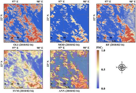
Figure 4.
FSC mapping comparison among five algorithms retrieved from the Landsat OLI (OLI), MOD10A1 (MOD) and random forest (RF), support vector machine (SVM) and back-propagation artificial neural network (ANN).
4.3. Accuracy Verification
Figure 5 shows that the BP-ANN and SVM models perform worse than the RF model and MOD10A1 in forestland and shrubland; moreover, these two models tend to overestimate the FSC more than the RF model and MOD10A1, and the RMSE is larger than 0.3. In particular, the RMSE of the BP-ANN in bare land reaches 0.34. In contrast, MOD10A1 performs worse in grassland, cropland and other lands. However, the RF performs best among the three machine learning models. In each land cover type except forestland, MOD10A1 underestimates the FSC in comparison with the Landsat OLI. The FSC distributions of the three machine learning models are close to those of the Landsat OLI in each land cover type; the AE of the RF model is especially good, between −0.07 and 0.05. However, the BP-ANN and SVM overestimate the FSC in forestland and shrubland, and the AE is larger than 0.3 for both models. The PAE of the RF model is the lowest, and the NAE of the BP-ANN is the lowest over each land cover type. Overall, the RF model performs the best among the other machine learning models on the TP; the RMSE, AE, PAE and NAE of the RF model are all lower than those of the other models, with average values of 0.23, 0.01, −0.17 and 0.15, respectively. In particular, the RF model performs better in forestland and shrubland, with RMSEs of only 0.13 and 0.18, respectively. Table 3 shows the overall accuracy of each FSC inversion model in the TP. These results further confirm that the three machine learning models overestimate the FSC and that MOD10A1 underestimates the FSC in the TP.
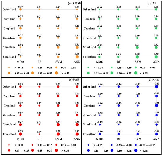
Figure 5.
Accuracy assessment including for FSC retrieved from the MOD10A1 (MOD) and random forest (RF), support vector machine (SVM), and back-propagation artificial neural network (ANN) using Landsat OLI. The root mean square error (RMSE), average error (AE), positive average error (PAE) and negative average error (NAE) were adopted to evaluate the FSC models.
Table 3.
Error evaluation of MOD10A1 (MOD), random forest (RF), support vector machine (SVM) and back-propagation artificial neural network (ANN).
Figure 6 shows the average accuracy of each FSC inversion model in the TP. The results show that the RF model performs best in forestland, shrubland and grassland, with ACCs of 0.92, 0.89 and 0.84, respectively. In cropland and other lands, the BP-ANN model performs best with ACCs of 0.87 and 0.90, respectively. In bare land, MOD10A1 performs best with an ACC of 0.84. However, in forestland and shrubland, the BP-ANN model performs the worst with ACCs of 0.61 and 0.65, respectively. The overall ACCs are shown in Table 4. Combined with Figure 6, these results further indicate that the RF model is more suitable than the other models and that the MOD10A1 product for inverting the FSC in the TP has an overall ACC of 0.84.
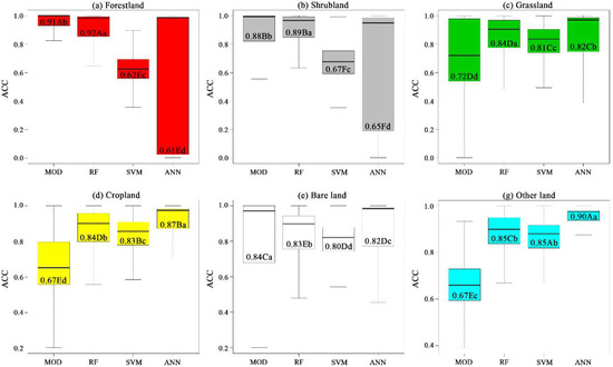
Figure 6.
Boxplots of the accuracy distributions of MOD10A1 (MOD), random forest (RF), support vector machine (SVM) and back-propagation artificial neural network (ANN) under different land cover types over the Tibetan Plateau. Labels are composed of the average accuracy and the results of the significance tests (in the case of p < 0.05). The uppercase letters represent the accuracy of the specific model from high to low (A to D) among different land cover types, while the lowercase letters represent the accuracy from high to low (a to d) among the four FSC models for each land cover type.
Table 4.
Overall average accuracy (ACC) of MOD10A1 (MOD), random forest (RF), support vector machine (SVM) and back-propagation artificial neural network (ANN) over the Tibetan Plateau.
To explore the accuracy of each model under different FSC gradients, the verified pixels are divided into four classes based on snow maps retrieved from Landsat OLI, namely, areas with low values (FSC between 0% and 25%), medium-low values (FSC between 25% and 50%), medium-high values (FSC between 50% and 75%), and high values (FSC between 75% and 100%). Figure 7 shows the accuracy distributions of each FSC model under various fractional snow cover gradients over the Tibetan Plateau. Results indicate that the effects of FSC gradients on each model are different. From areas with low FSC values to high FSC values, the ACC of MOD10A1 decreases significantly. The ACCs of RF and BP-ANN in areas with low and high FSC values are higher than those in areas with medium FSC values. For the SVM, the ACC in areas with medium FSC values is higher than that in areas with low and high FSC values. In low-FSC areas, MOD10A1 performs the best with an ACC of 0.95, whereas the SVM performs the worst with an ACC of only 0.78. In areas with medium-low and medium-high FSC values, the SVM model performs best with a combined ACC of 0.85. However, the BP-ANN and MOD10A1 perform the worst in areas with medium-low and medium-high FSC values with ACCs of 0.50 and 0.59, respectively. In high FSC areas, the BP-ANN model performs the best, and the ACC reaches 0.94; however, the ACC of MOD10A1 in high FSC areas is only 0.53. Nevertheless, the RF model does not exhibit outstanding performance under any FSC gradient; instead, the RF model displays relatively stable performance under all FSC gradients.
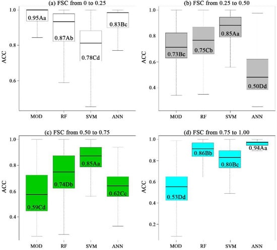
Figure 7.
Boxplots of the accuracy distributions of MOD10A1 (MOD), random forest (RF), support vector machine (SVM) and back-propagation artificial neural network (ANN) under various fractional snow cover gradients over the Tibetan Plateau. Labels are composed of the average accuracy and the results of the significance tests (in the case of p < 0.05). The uppercase letters represent the accuracy of the specific model from high to low (A to F) among different FSC gradients, while the lowercase letters represent the accuracy from high to low (a–d) among the four FSC models for each gradient.
Analysis of variance (F-test) between samples is an important process to verify whether the model accuracy obtained under different conditions is statistically significant. The land cover types and FSC gradients have significant influences on the model accuracy (p < 0.05) (Figure 6 and Figure 7). The results show that the accuracies of the three machine learning models are significantly higher than that of MOD10A1; therefore, these machine learning algorithms can significantly improve the FSC mapping accuracy relative to the linear regression algorithm employed by MOD10A1.
The effects of the land cover type and FSC gradient on the accuracy of each FSC inversion model in this study are combined. Figure 8 demonstrates that the effects of forestland and shrubland on the FSC inversion of each model are the same; similarly, the influences of grassland, cropland, bare land and other lands on the FSC inversion of each model are also the same. Overall, in forestland and shrubland, MOD10A1 and the RF model provide FSC distributions that are closer to those derived from Landsat OLI, while the SVM and BP-ANN models overestimate the FSC. In grassland, cropland, bare land and other lands, the FSC distributions from the RF model, SVM model and BP-ANN model are close to the Landsat OLI FSC; however, MOD10A1 underestimates the FSC compared to Landsat OLI.
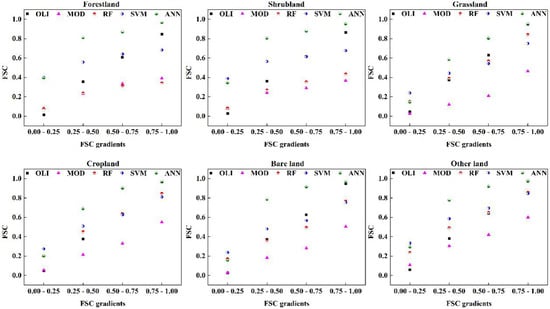
Figure 8.
FSC comparisons among Landsat OLI (OLI), MOD10A1 (MOD) and random forest (RF), support vector machine (SVM) and back-propagation artificial neural network (ANN) under various land cover types and FSC gradients.
Furthermore, the agreement between MOD10A1 and Landsat OLI decreases with an increase in the FSC for each land cover type. Similarly, the agreement between the RF model and Landsat OLI decreases with increasing FSC in forestland and shrubland, and the reverse FSC trend becomes closer to the Landsat OLI FSC distribution in other land cover types. The SVM overestimates the FSC in forestland and shrubland when the FSC is smaller than 50% and exhibits an underestimation trend when the FSC is larger than 50% in each land cover type. Overall, the BP-ANN overestimates the FSC in each land cover type.
5. Discussion
Although the accuracy of MOD10A1 is high in Europe, America and other regions, many problems are still encountered when adapting to the complex terrain of the TP. Accordingly, the complexity of snow monitoring throughout the TP has resulted in considerable challenges to important work involving the determination of snow cover. However, in recent years, with the introduction of machine learning and high-precision UAV data, the combination of these technologies has become an effective way to improve the accuracy of snow monitoring in mountainous areas with complex terrain, such as the TP.
The introduction of the BP-ANN algorithm into the FSC inversion for the Heihe River basin improved the FSC inversion accuracy compared with the MODIS global daily FSC product [26]. In addition, the RF method was employed in a snow depth inversion model based on passive microwave data in the Reynolds Creek Mountains, and the results demonstrated that the RMSE of the snow depth compared with ground-based observations declined to 0.09 m [40]. The SVM algorithm is also capable of accurately extracting and distinguishing areas with dry snow, wet snow and no snow in permafrost regions [41]. The SVM algorithm was further found to be able to extract snow information in mountainous areas with sufficient accuracy [42].
In this study, different machine learning models were employed for FSC inversion and compared with the global MODIS daily snow cover product. The results indicated that the accuracy of the machine learning algorithms is better than that of the MOD10A1 product in the TP. Among the three machine learning models used in this study, the RF model performed with ideal efficiency and accuracy in the FSC inversion over the TP with complex terrain, especially in forestland and shrubland. However, these machine learning models generally exhibit inconsistent performance under different FSC gradients, mainly as a result of the algorithm structure. Although the BP-ANN has a strong self-learning ability [43], its defects are obvious. First, the BP-ANN algorithm constitutes a local search optimization method that easily falls into local extrema, which leads to training failure [44]. Second, no unified and complete theoretical guidance has been developed for selecting the network structure; consequently, the network parameters can be selected only by experience. Unfortunately, the structure of the network directly affects its training and prediction abilities [45]. In this study, the improvement of the training ability exceeded a certain threshold, but the prediction ability decreased; that is, the so-called overfitting phenomenon appeared, which was mainly due to an excessive number of neurons [46,47]. Hence, the BP-ANN performed worse in the transition zone between areas with snow and no snow and overestimated the FSC in regions with fragmented snow cover. In contrast, nonlinear mapping constitutes the theoretical basis of the SVM algorithm, which uses an inner-product kernel function instead of nonlinear mapping to a high-dimensional space [48]. However, while the SVM model is mature in dealing with classification problems, the SVM algorithm still needs to be improved for regression problems and still encounters some difficulties when faced with large sample datasets. Moreover, the algorithm often fails due to storage and computation defects [49]. Finally, in the RF model, each tree randomly selects some samples and some features to avoid overfitting; consequently, the model features a good anti-noise ability and stable performance [50,51]. Furthermore, the RF model can handle very high-dimensional data and omit the work associated with feature selection [52].
Traditional remote sensing on the FSC inversion mainly includes two methods: the linear regression and spectral mixture analysis algorithms. However, previous studies have shown that these two algorithms perform worse in the Tibetan Plateau because of snow heterogeneity [24,25]. According to statistics, the average snow depth of the ground observations is around 5 cm so it is difficult to monitor the snow cover accurately by using remote sensing because the snow is shallow in the Tibetan Plateau [53]. The strong solar radiation, wind-blown snow, and the rugged terrain are the main reasons causing the snow to be patchy [10,35]. This study concludes that the machine learning algorithm can obtain satisfactory FSC inversion accuracy over complex terrain and regions with fragmented snow distribution in the TP. Specifically, the RF model displays acceptable accuracy when snow is patchy, and also robustness under different land cover types. However, machine learning is a form of artificial intelligence, which itself belongs to the scope of computer science. There are limitations to the interpretability of computing processes, which is referred to as the so-called “black box” of artificial intelligence. Further understanding of the snow radiation characteristics and distribution pattern, making the selection of variables that affect the FSC inversion is completely controllable. Machine learning can carry out optimized simulations based on the selected variables, avoiding the influence of human factors on model construction. Therefore, machine learning provides a reliable choice for snow cover inversion based on remote sensing in mountainous areas. However, how to obtain more effective input variables to improve the efficiency of machine learning requires more work.
6. Conclusions
In this study, three kinds of FSC machine learning models, including RF, SVM and BP-ANN models, are trained and compared based on MODIS, UAV and other auxiliary data. Then, the fitting ability is evaluated using the 10-fold cross-validation method with Landsat 8 OLI data under various land cover and FSC gradients. The results indicate that introducing a highly accurate UAV-acquired snow map as a reference into a machine learning model can significantly improve the MODIS FSC mapping accuracy. The main conclusions are as follows:
- (1)
- Compared with MOD10A1, the machine learning FSC algorithms employed in this study can significantly improve the FSC mapping accuracy. The FSC distributions generated by the three machine learning models are close to (or slightly overestimate) the real FSC obtained by Landsat. However, MOD10A1 severely underestimates the FSC in the TP.
- (2)
- The land cover type is the main factor affecting the FSC inversion accuracies of the machine learning algorithms and MOD10A1. Machine learning algorithms can significantly reduce the effects of different land cover types on the extraction of FSC using MODIS. In particular, the RF algorithm significantly improves the FSC extraction accuracy in forestland and shrubland. The RMSEs of the RF model in forestland and shrubland are only 0.13 and 0.18, respectively, whereas the corresponding MOD10A1 RMSEs are 0.21 and 0.23, respectively.
- (3)
- Various FSC gradients also affect the FSC inversion accuracy. The accuracy of MOD10A1 decreases with an increasing FSC gradient. The accuracies of the three machine learning models also change with the FSC gradient, although they still achieve acceptable accuracy compared to MOD10A1. Ultimately, the RF model performs the best with the most stable accuracy among the three machine learning models.
- (4)
- Finally, the RF algorithm shows high accuracies, which are normally unaffected by changes in the land cover types and FSC gradients in the TP. Therefore, this study proposed that the RF algorithm is the most effective method for resolving the problems associated with fragmented snow cover in the complex terrain of the TP. Hence, using the RF model can improve the FSC inversion accuracy from MODIS data compared with MOD10A1.
Author Contributions
All authors contributed significantly to this manuscript. X.H. designed this study and provided editorial advice and feedback on the manuscript. C.L. performed the data analysis and prepared the manuscript, and X.L. helped the data analysis. Professor T.L. helped with the manuscript preparation. All authors have read and agreed to the published version of the manuscript.
Funding
This research was funded by Natural Science Foundation of China, grant number 41971293 and 41671330; the Science and Technology Basic Resource Investigation Program of China, grant number 2017FY100501; and the Startup Foundation for Introducing Talent of Nanjing University of Information Science & Technology (20191017).
Acknowledgments
Three anonymous reviewers made valuable contributions to, and helped clarify, our manuscript; and we thank Lingxiao Wang and Hui Liang for contributions to the data and figures.
Conflicts of Interest
The authors declare no conflicts of interest.
References
- Barnett, T.P.; Adam, J.C.; Lettenmaier, D.P. Potential impacts of a warming climate on water availability in snow-dominated regions. Nature 2005, 438, 303–309. [Google Scholar] [CrossRef] [PubMed]
- Domine, F.; Barrere, M.; Sarrazin, D.; Samuel, M. Automatic monitoring of the effective thermal conductivity of snow in a low-Arctic shrub tundra. Cryosphere 2015, 9, 1633–1665. [Google Scholar] [CrossRef]
- Bair, E.H.; Davis, R.E.; Dozier, J. Hourly mass and snow energy balance measurements from Mammoth Mountain, CAUSA, 2011–2017. Earth Syst. Sci. Data 2018, 10, 549–563. [Google Scholar] [CrossRef]
- Zhao, P.; Zhou, Z.J.; Liu, J.P. Variability of Tibetan spring snow and its associations with the hemispheric extratropical circulation and east Asian summer monsoon rainfall: an observational investigation. J. Clim. 2007, 20, 3942–3955. [Google Scholar] [CrossRef]
- Qian, Y.F.; Zheng, Y.; Zhang, Y. Responses of China’s summer monsoon climate to snow anomaly over the Tibetan Plateau. Int. J. Climatol. 2003, 23, 593–613. [Google Scholar] [CrossRef]
- Wu, Z.W.; Zhang, P.; Chen, H. Can the Tibetan Plateau snow cover influence the interannual variations of Eurasian heat wave frequency? Clim. Dyn. 2016, 46, 3405–3417. [Google Scholar] [CrossRef]
- Wang, S.Y.; Wang, X.Y.; Chen, G.S. Complex responses of spring alpine vegetation phenology to snow cover dynamics over the Tibetan Plateau, China. Sci. Total Environ. 2017, 593–594, 449–461. [Google Scholar] [CrossRef] [PubMed]
- Wang, X.Y.; Wu, C.Y.; Peng, D.L. Snow cover phenology affects alpine vegetation growth dynamics on the Tibetan Plateau: Satellite observed evidence, impacts of different biomes, and climate drivers. Agric. For. Meteorol. 2018, 256–257, 61–74. [Google Scholar] [CrossRef]
- Wang, W.; Liang, T.G.; Huang, X.D.; Feng, Q.S.; Xie, H.J.; Liu, X.Y.; Chen, M.; Wang, X.H. Early warning of snow-caused disasters in pastoral areas on the Tibetan Plateau. Nat. Hazards Earth Syst. Sci. 2013, 13, 1411–1425. [Google Scholar] [CrossRef]
- Huang, X.D.; Deng, J.; Wang, W.; Feng, Q.S.; Liang, T.G. Impact of climate and elevation on snow cover using integrated remote sensing snow products in Tibetan Plateau. Remote Sens. Environ. 2017, 190, 274–288. [Google Scholar] [CrossRef]
- Hao, X.H.; Luo, S.Q.; Che, T.; Wang, J.; Li, H.Y.; Dai, L.Y.; Huang, X.D.; Feng, Q.S. Accuracy accessment of four cloud-free snow cover porducts over the Qinghai-Tibetan Plateau. Int. J. Digit. Earth 2018, 12, 375–393. [Google Scholar] [CrossRef]
- Zhang, Y.; Huang, X.D.; Wang, W.; Liang, T.G. Validation and Algorithm Redevelopment of MODIS Daily Fractional Snow Cover Products. Arid Zone Res. 2013, 30, 808–814. (In Chinese) [Google Scholar]
- Hall, D.K.; Riggs, G.A.; Salomonson, V.V. Development of methods for mapping global snow cover using moderate resolution imaging spectroradiometer data. Remote Sens. Environ. 1995, 54, 127–140. [Google Scholar] [CrossRef]
- Hao, X.H.; Wang, J.; Wang, J.; Huang, X.D.; Li, H.Y.; Liu, Y. Observations of Snow Mixed Pixel Spectral Characteristics Using a Ground-Based Spectral Radiometer and Comparing with Unmixing Algorithms. Spectrosc. Spectr. Anal. 2012, 32, 2753. (In Chinese) [Google Scholar]
- Brown, R.D.; Robinson, D.A. Northern Hemisphere spring snow cover variability and change over 1922–2010 including an assessment of uncertainty. Cryosphere 2011, 219–229. [Google Scholar] [CrossRef]
- Hori, M.; Sugiura, K.; Kobayashi, K.; Aoki, T.; Tanikawa, T.; Kuchiki, K.; Niwano, M.; Enomoto, H. A 38-year (1978–2015) Northern Hemisphere daily snow cover extent product derived using consistent objective criteria from satellite-borne optical sensors. Remote Sens. Environ. 2017, 191, 402–418. [Google Scholar] [CrossRef]
- Metsämäki, S.; Pulliainen, J.; Salminen, M.; Luojus, K.; Wiesmann, A.; Solgerg, R.; Böttcher, K.; Hiltunen, M.; Ripper, E. Introduction to GlobSnow Snow Extent products with considerations for accuracy assessment. Remote Sens. Environ. 2015, 156, 96–108. [Google Scholar] [CrossRef]
- Schattan, P.; Schwaizer, G.; Schöber, J.; Achleitner, S. The complementary value of cosmic-ray neutron sensing and snow covered products for snow hydrological modelling. Remote Sens. Environ. 2020, 239, 111603. [Google Scholar] [CrossRef]
- Nagler, T.; Rott, H.; Ripper, E.; Bippus, G.; Hetzenecker, M. Advancements for snowmelt monitoring by means of Sentinel-1 SAR. Remote Sens. 2016, 8, 348. [Google Scholar] [CrossRef]
- Simic, A.; Fernandes, R.; Brown, R.; Romanov, P.; Park, W. Validation of vegetation, MODIS, and GOES + SSM/ I snow cover products over Canada based on surface snow depth observations. Hydrol. Process. 2004, 18, 1089–1104. [Google Scholar] [CrossRef]
- Liang, T.G.; Huang, X.D.; Wu, C.X.; Liu, X.Y.; Li, W.D.; Guo, Z.G.; Ren, J.Z. An application of MODIS data to snow cover monitoring in a pastoral area: A case study in Northern Xinjiang, China. Remote Sens. Environ. 2008, 112, 1514–1526. [Google Scholar] [CrossRef]
- Wang, W.; Huang, X.D.; Deng, J.; Xie, H.J.; Liang, T.G. Spatio-temporal change of snow cover and its response to climate over the Tibetan Plateau based on an improved daily cloud-free snow cover product. Remote Sens. 2015, 7, 169–194. [Google Scholar] [CrossRef]
- Yu, J.Y.; Zhang, G.Q.; Yao, T.D.; Xie, H.J.; Zhang, H.B.; Ke, C.Q.; Yao, R.Z. Developing daily cloud-free snow composite products from MODIS Terra-Aqua and IMS for the Tibetan Plateau. IEEE Trans. Geosci. Remote Sens. 2016, 54, 2171–2180. [Google Scholar] [CrossRef]
- Zhang, Y.; Huang, X.D.; Hao, X.H.; Wang, J.; Wang, W.; Liang, T.G. Fractional snow-cover mapping using an improved endmember extraction algorithm. J. Appl. Remote Sens. 2014, 8, 084691. [Google Scholar] [CrossRef]
- Liang, H.; Huang, X.D.; Sun, Y.H.; Wang, Y.L.; Liang, T.G. Fractional snow-cover mapping based on MODIS and UAV data over the Tibetan Plateau. Remote Sens. 2017, 9, 1332. [Google Scholar] [CrossRef]
- Hou, J.L.; Huang, C.L. An application of ANN for mountainous snow cover fraction mapping with MODIS and ancillary topographic data. Geosci. Remote Sens. Symp. 2014, 14058963. [Google Scholar]
- Czyzowska, E.H.; Leeuwen, W.J.; Hirschboeck, K.K. Fractional snow cover estimation in complex alpine-forested environments using an artificial neural network. Remote Sens. Environ. 2015, 156, 403–417. [Google Scholar] [CrossRef]
- Ge, J.; Meng, B.P.; Yang, S.X. Dynamic monitoring of alpine grassland coverage based on UAV technology and MODIS remote sensing data—A case study in the headwaters of the Yellow River. Acta Pratacult. Sin. 2017, 26, 1–12. (In Chinese) [Google Scholar]
- Wang, X.Y.; Jian, W.; Che, T.; Huang, X.D.; Hao, X.H.; Li, H.Y. Snow Cover Mapping for Complex Mountainous Forested Environments Based on a Multi-Index Technique. IEEE J-STARS 2018, 11, 1433–1441. [Google Scholar] [CrossRef]
- Yang, D.; Zhou, C.; Zhou, H.O.; Chen, C. Characteristics of Variation in Runoff across the Nyangqu River Basin in the Qinghai-Tibet Plateau. J. Resour. Ecol. 2012, 3, 80–86. [Google Scholar]
- Chang, Q.F.; Lai, Z.P.; An, F.Y. Chronology for terraces of the Nalinggele River in the north Qinghai-Tibet Plateau and implications for salt lake resource formation in the Qaidam Basin. Quat. Int. 2016, 430, 12–20. [Google Scholar] [CrossRef]
- Damien, S.M.; Friedl, M.A. User Guide to Collection 6 MODIS Land Cover (MCD12Q1 and MCD12C1) Product; USGS: Reston, VA, USA, 2018. [CrossRef]
- Hall, D.K.; Riggs, G.A. MODIS/Terra Snow Cover Daily L3 Global 500 m SIN Grid, 6th ed.; NASA Natinal Snow and Ice Data Center: Boulder, CO, USA, 2016. [Google Scholar] [CrossRef]
- He, Q. Neural Network and its Application in IR; Graduate School of Library and Information Science, University of Illinois at Urbana-Champaign Spring: Champaign, IL, USA, 1999. [Google Scholar]
- Hao, S.R.; Jiang, L.M.; Shi, J.C.; Wang, G.X.; Liu, X.J. Assessment of MODIS-Based Fractioal Snow Cover Products Over the Tibetan Plateau. IEEE J. Sel. Top. Appl. Earth Observ. Remote Sens. 2018, 99, 1–16. [Google Scholar]
- Tiryaki, S.; Aydın, A. An artificial neural network model for predicting compression strength of heat treated woods and comparison with a multiple linear regression model. Constr. Build. Mater. 2014, 62, 102–108. [Google Scholar] [CrossRef]
- Breiman, L. Random Forests. Mach. Learn. 2001, 45, 5–32. [Google Scholar] [CrossRef]
- Verrelst, J.; Camps, V.G.; Muñoz-Marí, J. Optical remote sensing and the retrieval of terrestrial vegetation bio-geophysical properties-A review. ISPRS-J. Photogramm. Remote Sens. 2015, 108, 273–290. [Google Scholar] [CrossRef]
- Johnson, B. Scale Issues Related to the Accuracy Assessment of Land Use/Land Cover Maps Produced Using Multi-Resolution Data: Comments on “The Improvement of Land Cover Classification by Thermal Remote Sensing”. Remote Sens. 2015, 7, 8368–8390. [Google Scholar] [CrossRef]
- Tinkham, W.T.; Smith, A.M.S.; Marshall, H.P. Quantifying spatial distribution of snow depth errors from LiDAR using Random Forest. Remote Sens. Environ. 2014, 141, 105–115. [Google Scholar] [CrossRef]
- Longepe, N.; Shimada, M.; Allain, S.; Pottier, E. Capabilities of Full-Polarimetric PALSAR/ALOS for Snow Extent Mapping. IEEE Int. Geosci. Remote Sens. Symp. 2008, 4, 1026–1029. [Google Scholar]
- Zhu, L.; Xiao, P.; Feng, X. Support vector machine-based decision tree for snow cover extraction in mountain areas using high spatial resolution remote sensing image. J. Appl. Remote Sens. 2014, 8, 084698. [Google Scholar] [CrossRef]
- Ding, S.; Su, C.; Yu, J. An optimizing BP neural network algorithm based on genetic algorithm. Artif. Intell. Rev. 2011, 36, 153–162. [Google Scholar] [CrossRef]
- Ma, N.; Ma, G.; Li, C. Implementation of Modification Algorithm for BP Network Local Minima. J. North China Inst. Aerosp. Eng. 2007, 17, 24–27. (In Chinese) [Google Scholar]
- Li, J.; Qin, J.; Wen, X.; Hu, Y. Over-Fitting in Neural Network Learning Algorithms and Its Solving Strategies. J. Vib. Meas. Diagn. 2002, 22, 260–264. (In Chinese) [Google Scholar]
- Minns, A.W.; Hall, M.J. Artificial neural networks as rainfall-runoff models. Hydrol. Sci. J. 1996, 41, 399–417. [Google Scholar] [CrossRef]
- Liu, Y.; Chen, Y.; Hu, J.; Qin, H.; Wang, Y. Long-Term Prediction for Autumn Flood Season in Danjiangkou Reservoir Basin Based on OSR-BP Neural Network. In Proceedings of the 2010 Sixth International Conference on Natural Computation (ICNC 2010), Yantai, China, 10–12 August 2010; pp. 1717–1720. [Google Scholar]
- Doucet, J.P.; Barbault, F.; Xia, H. Nonlinear SVM Approaches to QSPR/QSAR Studies and Drug Design. Curr. Comput.-Aided Drug Des. 2007, 3, 263–289. [Google Scholar] [CrossRef]
- Xie, F. Support Vector Machine and Application Research. J. Anhui Inst. Educ. 2007, 25, 56–59. (In Chinese) [Google Scholar]
- Ma, L.; Fan, S. CURE-SMOTE algorithm and hybrid algorithm for feature selection and parameter optimization based on random forests. BMC Bioinform. 2017, 18, 169. [Google Scholar] [CrossRef]
- Zhang, X.; Lin, X.; Zhao, J. Efficiently Predicting Hot Spots in PPIs by Combining Random Forest and Synthetic Minority Over-sampling Technique. IEEE-ACM Trans. Comput. Biol. Bioinform. 2018, 16, 774–781. [Google Scholar] [CrossRef]
- Bernard, S.; Heutte, L.; Adam, S. Forest-RK: A New Random Forest Induction Method. ICIC 2008, 5227, 430–437. [Google Scholar]
- Wang, Y.L.; Huang, X.D.; Wang, J.S.; Zhou, M.Q.; Liang, T.G. AMSR2 snow depth downscaling algorithm based on a multifactor approach over the Tibetan Plateau, China. Remote Sens. Environ. 2019, 231, 111268. [Google Scholar] [CrossRef]


© 2020 by the authors. Licensee MDPI, Basel, Switzerland. This article is an open access article distributed under the terms and conditions of the Creative Commons Attribution (CC BY) license (http://creativecommons.org/licenses/by/4.0/).