Abstract
Since the implementation of the great western development strategy in 2000, the ecological environment in the western region of China has been significantly improved. In order to explore the temporal and spatial characteristics of vegetation coverage in the western region, this paper adopted the method of Maximum Value Composite (MVC) to obtain the mean Normalized Difference Vegetation Index (NDVI) of vegetation on the basis of the Moderate-resolution Imaging Spector audiometer (MODIS) data of 2000/2005/2010/2015/2018. Thereafter, the spatio-temporal differentiation characteristics of vegetation in western China were analyzed. The results show that: (1) According to the time characteristics of vegetation coverage in the western region, the average annual NDVI value of vegetation coverage in the growing season in the western region fluctuated between 0.12 and 0.15, among which that of 2000 to 2010 fluctuated more greatly but did not show obvious change trend. (2) Based on Sen trend and Mann-Kendall test analysis, the area of vegetation coverage improvement in the western region from 2000 to 2018 was larger than that of significant vegetation degradation. (3) From the perspective of global autocorrelation coefficient, Moran’s I values were all positive from 2000 to 2018, which indicates that the vegetation coverage in the west showed strong positive autocorrelation in each period. According to the average value and coefficient of variation of vegetation coverage, the vegetation coverage was lower in 2000, its internal variation was smaller, and the vegetation coverage increased with time. According to the local spatial autocorrelation analysis, the vegetation coverage levels in different regions varied greatly. (4) The standard deviation ellipse method was used to study the spatial distribution and directional transformation of vegetation. It makes the result more intuitive, and the three levels of gravity center shift, direction shift, and angle shift were considered: the vegetation growth condition in the spatial aggregation area improved in 2015; the standard deviation ellipses in 2000 and 2018 overlapped and shifted eastward, which indicates that the vegetation coverage conditions in the two years were similar and got ameliorated.
1. Introduction
In the international approaches to vegetation degradation, generally Remote Sensing (RS), Global Position System (GPS), and Geographic Information System (GIS) are combined to monitor vegetation degradation. For example, Mustafa [1] studied the evaluation method of vegetation degradation in abandoned coal mines using spatial information technology and analyzed the vegetation degradation status before and after coal mining. Anilz Chitade [2] et al. analyzed the land use/cover changes of coal mines in Chandpur District of India from 1990 to 2010. Bao Nisha [3] monitored and compared the different time zones of mining production by analyzing the changes of land use, reclamation area and vegetation coverage. Vegetation is the most important part of land cover and plays a very important role in conserving soil, regulating atmosphere, and maintaining the stability of the ecological system [4,5]. Research on vegetation dynamics plays an important role in land cover research. Normalized vegetation index, as the best indicator of vegetation growth and vegetation coverage [6] which could reflect vegetation coverage information with a high spatial-temporal scale, is widely used in ecological, environmental, and agricultural fields [6,7].
With the progress of remote sensing and Geographic Information System (GIS) technology, images with different sensors and multiple spatial and temporal resolutions can be fused, and remote sensing image processing software and GIS technology can be integrated and applied. Subsequently, vegetation degradation assessment and monitoring technologies based on remote sensing and GIS have also developed and matured [8,9,10]. As the main component of ecosystem, vegetation is the “indicator” of global change research, and is also the key research field of ecology, geography, and other disciplines. Vegetation coverage refers to the percentage of the vertical projection area of vegetation (branches, stems, and leaves) on the ground to the total area of the statistical area, which is one of the important parameters to characterize the quality of land vegetation and the growth dynamics of vegetation communities, and is also a comprehensive quantitative indicator of the land cover status of plant communities [11,12]. Remote sensing technology can extract many vegetation parameters such as surface coverage and vegetation coverage from multi-scale, multi-temporal, and multi-band remote sensing images, and has become an important means to study the spatial distribution and dynamic evolution of vegetation [13].
Compared with the international circle, based on the study of vegetation coverage, Chinese scholars have used the comprehensive information evaluation model to extract and evaluate the degree of vegetation degradation [14]. Through rapid extraction of information on soil erosion, land desertification and land salinization, the general situation of vegetation degradation was depicted, and the risk of vegetation degradation was graded and evaluated [15,16,17]. In terms of research methods, scholars use linear trend method, R/S analysis method, spatial interpolation method, spatial autocorrelation, standardized ellipse, etc., which is of important practical significance for vegetation and ecological environment protection in the research area [18]; besides, from the perspectives of climate change, remote sensing image interpretation, field vegetation survey and vegetation degradation characteristics and laws in mining areas [19], scholars analyzed the dynamic evolution of vegetation at different spatial scales by path analysis and other mathematical statistics and spatial analysis methods [20,21].
In this study, some western provinces were selected as the research area. Based on Moderate-resolution Imaging Spector adiometer (MODIS) data in the growing season of 2000/2005/2010/2015/2018 and the existing vegetation spatial differentiation methods at home and abroad, Sen trend analysis and Mann-Kendall test method were applied to analyze the spatial and temporal pattern change trend of vegetation degradation in west China, and then spatial autocorrelation and standard deviation ellipse (SDE) methods were used to analyze the spatial aggregation correlation of vegetation coverage and geographic spatial distribution of gravity center shift of vegetation. Thereby, the dynamic change law of vegetation in the western region were revealed more comprehensively, thus locating the background status for the later analysis of the influencing factors of vegetation degradation, providing basis for vegetation restoration and ecological environment protection in the western region, and providing reference and a scientific basis for vegetation degradation monitoring and decision-making of degraded land remediation in west China.
2. Data and Methods
2.1. Study Area
The western region of China is located in the eastern part of Eurasia, with vast territory, complicated geology, small population, backward economy, and blocked traffic. It is an underdeveloped area in China and needs to be further developed. Since the reform and opening, with the scale of mineral resources development being continuously increased in the 12 western provinces (Figure 1), they have increasingly become the main area of mineral resources development in China. At the end of 2010, the country’s coal reserves were ascertained to be 1341.2 billion tons, an increase of about 300 billion tons over 2005, with the western region accounting for more than 90% of the national increase [22,23]. According to the following pictures of the typical surveyed areas (Figure 2), as the coal resources in the central and eastern regions are drying up, coal development is accelerating to the west, where the ecological environment is fragile. Owing to the fragile ecological environment in the west, it faces the problem of relative imbalance between development and protection. Therefore, the vegetation coverage in west China is more susceptible to external disturbances. Analysis of the spatio-temporal variation characteristics of vegetation in this region is of great significance for evaluating its ecological environment and implementing reasonable control measures.
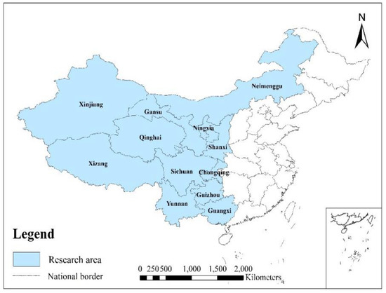
Figure 1.
Study Area.
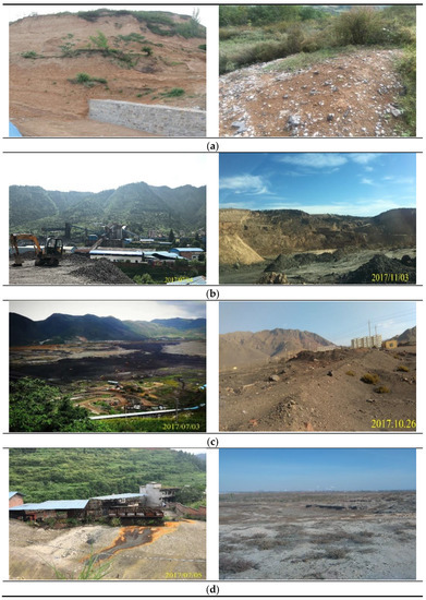
Figure 2.
The field survey typical pictures of the western region. Shaanxi xunyao mining area (a), Guizhou pan county mining area, and Inner Mongolia Pingzhuang mining area (b), Yunnan xiaolongtan mining area, and Xinjiang tuha mining area (c), Sichuan gushi mining area, and Ningxia lingwu mining area (d).
2.2. Data Sources and Processing
Since Normalized Difference Vegetation Index (NDVI) and EVI data developed by MODIS have different descriptions of high-density vegetation in humid environment, this feature of EVI data provides a new way to study the seasonal changes of high-coverage vegetation. EVI data is more closely related to the monthly average temperature, so EVI data can be used to study the relationship between vegetation and temperature in the later period. In this study, NDVI was selected as the data source for the western region of China, which have a similar ability to describe low-cover vegetation in the arid and sub-humid environment.
The remote sensing data are from the MOD13Q1 data of the vegetation growing season from May to September (from 129 days to 273 days), the 800 scenes, the 19th Issue, 2000-2018, United States Geological Survey (USGS) (https://search.earthdata.nasa.gov/search) with a spatial resolution of 250m and a temporal resolution of 16 days. Firstly, MODIS Reprojection Tool (MRT) software was used to convert the data format and projection, then MODIS NDVI image data for 2000/2005/2010/2015/2018 were obtained by cutting out the boundaries of 12 provinces in the west, and then The Environment for Visualizing Images (ENVI5.3) software was used to synthesize annual NDVI1 data and monthly NDVI1 data by Maximum Value Composite (MVC) to remove the influence of cloud, fog and solar altitude angle as much as possible. Since the annual maximum NDVI can effectively reflect the regional vegetation coverage, and the time point when the vegetation flourish is not easy to determine, the annual maximum NDVI1 of each pixel was selected as the research data. Finally, the Band Math operation expression (b1 It 0) * 0 + (b1 ge 0) * (b1 * 0.0001) was used to make NDVI1 value between 0 and 1. The Band Math operation expression of vegetation coverage((b1 lt 0.031766) * 0 + (b1 gt 0.522991) * 1 + (b1ge 0.031766 and b1 le 0.522991) * ((b1 − 0.031766)/(0.522991 − 0.031766) and the calculation method of annual maximum mean are as follows:
In the formula, Pi is the average of the monthly maximum NDVI of the pixels from May to September, n is the number of regional pixels, verage is the normalized coefficient of vegetation coverage, and the reference value is 0.0121165124 [24,25].
2.3. Sen Trend Analysis and Mann-Kendall Test
The non-parametric Sen trend method was used to calculate the change trend of vegetation coverage in west China. The advantage of Sen trend that it has no requirement on data distribution makes it suitable for analysis of missing data, which could reduce the interference of abnormal values, and get SEN by calculating the median value of the sequence [26].
In the formula, i and j represent year i and year j, respectively, Xi and Xj represent year i NDVI1 and year j NDVI1, respectively, β represents trend degree, and the value of β indicates the rise and fall of the vegetation trend. When β > 0, the time sequence shows an upward trend, while when β < 0, the time sequence shows a downward trend.
However, Sen cannot judge the significance of sequence trend by itself. Mann-Kendall statistical test was applied to test the significance of Sen trend. Mann-Kendall is a nonparametric statistical method [27,28]. The process of the trend checking method is as follows: for the sequence , the magnitude relation between Xi and Xj (set as s) in all dual values (between Xi and Xj, j > i) is first determined. The following assumptions are made: sgn0: the data in the sequence are randomly arranged, i.e., there is no significant trend; sgn1: the sequence has a monotone trend of increasing or decreasing. The inspection statistic S is calculated by Formula (3):
Statistic S is defined as follows:
In selecting inspection statistics, when n < 10, the statistic s is directly used for bilateral trend inspection; when n ≥ 10, the statistic s approximately follows the standard normal distribution, then z is used for trend inspection, and the z value is calculated by Formula (5):
In the formula, z is the standardized test statistic, the value range of statistic z is (−∞, +∞), S is the test statistic, n is the number of sequence samples, m is the number of knots (repeated data sets) in the sequence, ti is the width of the knots (the number of repeated data in group I of repeated data sets). Xi and Xj respectively represent the NDVI value in year i and year j. Given the significance level α, the critical value Z1-α/2 was found in the normal distribution table; when |Z| ≤ Z1α/2, the original assumption is accepted, that is, the trend is not significant; when |Z| > Z1α/2, the original assumption is rejected, i.e., the trend is significant. Then Z1α/2 = 1.96. When β > 0 and Z1α/2 > 1.96, the sequence shows a significant upward trend; when β > 0 and |Z| ≤ Z1α/2, the sequence shows an upward but insignificant trend; similarly, when β < 0 and Z1α/2 > 1.96, the sequence shows a significant downward trend; when β < 0 and |Z| ≤ Z1α/2, the sequence shows a downward but insignificant trend.
In this paper, the trend inspection was carried out by using the inspection statistic S. Given the significance level α, if |S| ≥ S α/2, W0 is not permitted to determine that the original sequence has a significant trend, otherwise W0 is permitted to determine that the sequence trend is not significant. If S > 0, the sequence is considered to have an upward trend; if S = 0, there is no trend; if S < 0, the sequence is considered to have a downward trend.
2.4. Spatial Autocorrelation
Spatial autocorrelation analysis can reveal the correlation between a certain regional unit and neighboring regional units in terms of common geographic features or attribute values [29,30] and can be analyzed from global and local perspectives. The commonly used spatial autocorrelation measure indexes are Moran’s I value and Local indication of spatial association (LISA) value. Global Moran’s I can reveal the global spatial correlation of vegetation coverage. Local Moran’s I index can reveal the local spatial aggregation characteristics of vegetation coverage in west China. Its essence is that the index is high, indicating similar spatial unit aggregation; otherwise, it indicates different spatial unit aggregation [31,32]. The calculation formula is as follows:
In the formula, n is the number of spatial units in the research area; Xi and Xj are the vegetation coverage (attribute values) of spatial units i and j respectively, is the average value of all the attribute values mentioned above; Wij is the spatial weight: S2 is the variance of vegetation coverage of each spatial unit (8); I is global Moran’s I and Ii is local LISA index. If I > 0, it is positive correlation; If I < 0, it is negative correlation; if the absolute value of I tends to be 1, there is strong spatial autocorrelation.
2.5. Standard Deviation Ellipse
Standard deviation ellipse (SDE) can reveal geographical spatial characteristics and spatio-temporal evolution from the perspectives of center of gravity, distribution range, direction and shape, etc. [33]. It is a method to accurately reveal various economic distribution characteristics by using spatial statistical methods. Its shape index (the ratio of the length of the minor axis to the major axis of the ellipse) reflects the shape of the distribution of elements. When the value is between 0 and 1, the closer it is to 1, the closer the shape of the main area where the spatial distribution of elements is to the standard circle, otherwise the closer it is to 0, the closer the shape is to linearity.
X and Y respectively represent the longitude and latitude coordinates of the vegetation coverage center; Xi and Yi respectively correspond to the longitude and latitude coordinates of vegetation coverage on grid i, and Mi represents the value of vegetation coverage grid i.
X-axis length and y-axis length of elliptic distribution:
Aazimuthal angle:
3. Results and Discussion
3.1. Temporal Variation Characteristics of Normalized Difference Vegetation Index (NDVI) in Growing Season of West China
In order to study the characteristics of NDVI changes with time in the growing season in the western region [34], the average NDVI values of the vegetation coverage areas in the annual NDVI images from 2000 to 2018 were taken to represent the vegetation coverage status in that year, and an inter annual NDVI change figure was made (Figure 3). As can be seen in Figure 3, the average annual NDVI value of the vegetation coverage area in the western region fluctuated between 0.12 and 0.15 during the growing season, among which the NDVI value of the vegetation coverage area fluctuated greatly from 2000 to 2010, and there was no obvious trend characteristic. However, since 2010, NDVI in the vegetation coverage area has shown a rapid growth trend, indicating that the overall growth of vegetation has begun to improve.
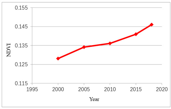
Figure 3.
Normalized Difference Vegetation Index (NDVI) changes of vegetation in growing season in west China in 2000/2005/2010/2015/2018.
3.2. An Analysis of the Spatial Variation Trend of NDVI in Growing Season in West China
The combination of Theil-Sen Median trend analysis and Mann-Kendall test [35] can effectively reflect the spatial distribution characteristics of vegetation NDVI change trend during the growing season in west China from 2000 to 2018. From Table 1, it can be seen that the vegetation activities in the western region were obviously degraded on the whole, and some areas were also improved. The vegetation degradation was obvious in 4.63% of the regions, the vegetation of 65.91% of the regions was degraded and relatively stable, the vegetation of 29.30% of the regions was improved, and the vegetation in 0.16% of the area has a significant improvement trend. From the above data, it can be seen that the change trend of vegetation NDVI in the growing season in the west showed a significant degradation trend, and some areas also began to develop towards an upward trend.

Table 1.
The NDVI (Normalized Difference Vegetation Index) of trend statistics.
Based on Sen’s trend analysis and Mann-Kendall test (M-Ktest), the change trend of NDVI on pixel scale was analyzed (Figure 4). According to the number of pixels, the degraded and stable regions account for the largest proportion, the significantly improved regions account for a smaller proportion, and the significantly degraded regions account for a smaller proportion than the slightly improved regions, indicating that vegetation degradation has ameliorated.
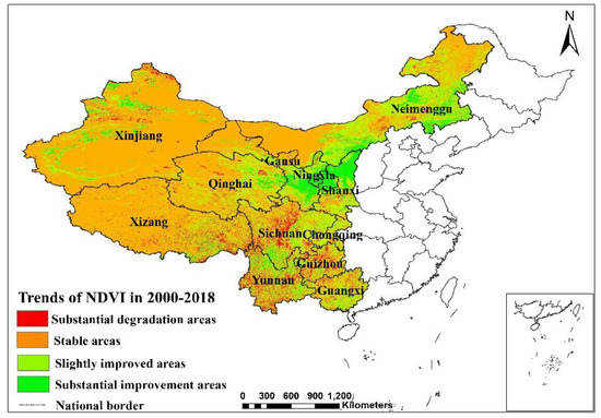
Figure 4.
Annual NDVI change trend of vegetation in the growing season of west China from 2000 to 2018.
As for the distribution area of vegetation degradation, there are many degraded pixels in northwest Qinghai, northwest Xinjiang, most of Tibet, and northern Sichuan; the regions with improved NDVI in the growing season in west China are mainly distributed in the southwest of Gansu, the central and southern regions of northern Shaanxi, the eastern region of Inner Mongolia, the northeast of Qinghai, the western part of Xinjiang, the southern part of Sichuan, the northern and eastern parts of Yunnan, the southern parts of Guizhou and Guangxi, and Chongqing; the eastern part of Xinjiang, the western part of Tibet, the northwestern part of Gansu, the western part of Qinghai, and the western part of eastern Mongolia showed a trend of degeneration, though were with little change and were relatively stable. According to the analysis of the above phenomena, the vegetation in the southwest and the south was in good condition and showed degraded pixels, which indicates that vegetation was affected by natural factors, such as temperature, precipitation and landform. The frequent occurrence of landslides and debris flows in the rainy season in the southwest made vegetation show degraded trend. Due to the implementation of the National Natural Forest Protection Project in recent years, the ecological environment has been improved to a great extent and the vegetation degradation has been improved. However, with the acceleration of urbanization, the rapid increase of population, and the need to improve infrastructure and management in the west, the restoration of vegetation cover has also been affected.
3.3. Spatial Correlation Analysis of Vegetation Coverage in Growing Season in West China
(1) Global aggregation feature analysis
With the help of the spatial autocorrelation Moran I tool in the analysis mode part of ArcGIS spatial statistics tool, the spatial autocorrelation coefficient Moran’s I value and related indexes of vegetation coverage in the western region in 2000, 2005, 2010, 2015, and 2018 are calculated as shown in Table 2:
Table 2.
Moran’s I mean and coefficient of variation of vegetation coverage.
Moran’ s I > 0 indicates a positive spatial correlation. The greater the value, the more obvious the spatial correlation is. Moran’s I < 0 indicates a negative correlation in the spatial region. The smaller the value, the greater the spatial difference is. Otherwise, if Moran’s I = 0, the space is at random. The aggregation characteristics of different administrative regions in the whole western vegetation coverage are available from the table. As far as the spatial autocorrelation coefficient of vegetation coverage is concerned, from 2000 to 2018, Moran’s I values were all positive numbers, the significance level of which can be determined by the p-value test of standardized Z values. Then comparing it with the significance level (α = 0.05) for it to pass the significance test (p < 0.01), rejecting the zero hypothesis, the research revealed that the vegetation coverage in west China showed strong positive autocorrelation in various periods [36]. That is to say, the vegetation coverage in west China is somehow characterized by the aggregation of similar characteristic values (high or low). Except 2015, Moran’s I value showed a slight downward trend from 2000 to 2018, Moran’s I decreased from 0.48828 to 0.47120 from 2000 to 2010, and from 0.47657 to 0.46430 from 2015 to 2018, indicating that the spatial autocorrelation of vegetation coverage in the western regions changed from strong to weak and the spatial aggregation of regions with similar vegetation coverage got weakened, which was mainly because the improvement in the overall growth of vegetation in west China from 2000 to 2015 and from 2015 to 2018 resulted in smaller differences in vegetation coverage among different regions.
According to the average value and coefficient of variation of vegetation coverage, from 2000 to 2005, the average value of vegetation coverage increased from 0.38973 to 0.40769, the coefficient of variation increased from 0.02674 to 0.02675, and the overall growth of vegetation coverage in the western region improved and the internal difference was not significant; from 2005 to 2010, the average value of vegetation coverage in the western region decreased from 0.40769 to 0.39809, and the coefficient of variation decreased from 0.02675 to 0.02661, indicating that the overall growth of vegetation coverage in the western region slowed down and the internal difference did not change much under the influence of natural or human factors at this stage; from 2010 to 2015, the average value of vegetation coverage in the west remained basically unchanged, with a slight increase in coefficient of variation, indicating that the overall growth of vegetation coverage in the west was relatively stable at this stage; from 2015 to 2018, the average value of vegetation coverage in the western region increased from 0.39807 to 0.40331, and the coefficient of variation decreased from 0.02665 to 0.02618, indicating that the overall growth of vegetation coverage in the western region became better and the internal difference was smaller at this stage. The average vegetation coverage in the growing season of the west in 2005 was 0.40769 and the coefficient of variation was 0.02675, both of which reached the maximum value in the testing year. By 2018, the average vegetation coverage was 0.40331 and in 2000, the average vegetation coverage was 0.38974, which was the minimum value in the testing years. Thus, we can see that the vegetation coverage was lower in 2000, but it increased with the passage of time, the vegetation growth status improved, and its internal variation became smaller [37,38,39].
(2) Local aggregation feature analysis
The changes of vegetation coverage from the previous checking point in the western region in 2000, 2005, 2010, 2015, and 2018 were calculated respectively, and the correlation analysis of spatial local aggregation pattern was carried out. The spatial local indication of spatial association (LISA) cluster diagram of vegetation coverage changes in the western region was drawn using ArcGIS [40,41]: (Figure 5).
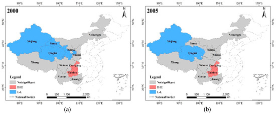
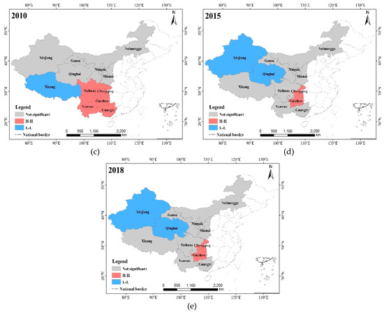
Figure 5.
LISA cluster diagram of vegetation coverage for western China in 2000 (a), 2005 (b), 2010 (c), 2015 (d), 2018 (e). Low-Low (L-L); High-High (H-H).
Analysis revealed that only Xinjiang, Gansu, Qinghai, Tibet, Sichuan, Chongqing, Guizhou, Yunnan, and Guangxi are the regional units showing significant aggregation types during the research period. In 2000, Xinjiang, Gansu and Qinghai showed L-L aggregation, while Chongqing and Guizhou showed H-H aggregation. By 2005, Gansu had become insignificant while other places remained unchanged. In 2010, Gansu Province also evolved into insignificant state, Tibet evolved into L-L aggregation type, and the H-H aggregation area added Sichuan, Yunnan, and Guangxi provinces on the basis of the previous two years, while the other places were insignificant. By 2015, Qinghai and Xinjiang were transformed from insignificant type to L-L aggregation areas, Chongqing and Guizhou were H-H aggregation areas, Sichuan, Yunnan, and Guangxi provinces were transformed into insignificant type. The vegetation aggregation areas in 2018 were exactly the same as those in 2015.
The discussion of the evolution characteristics of local aggregations came to the conclusion that the vegetation coverage levels in the western, southwestern and northwestern provinces were quite different. Among them, the western regions such as Xinjiang, Gansu, Qinghai, and Tibet were characterized by L-L aggregation; the southwest regions such as Sichuan, Chongqing, Guizhou, Yunnan, and Guangxi showed H-H aggregation characteristics; the northern Inner Mongolia region remained in an insignificant type for 5 years. Based on Sen’s trend analysis and Mann-Kendall test (M-K test), the change trend of NDVI on pixel scale was analyzed (Figure 4). According to the number of pixels, the degraded and stable regions account for the largest proportion, the significantly improved regions account for a smaller proportion, and the significantly degraded regions account for a smaller proportion than the slightly improved regions, indicating that vegetation degradation has ameliorated [42,43]; from 2000 to 2018, the vegetation coverage characteristics in Gansu Province changed from L-L aggregation to being insignificant, indicating that the vegetation degradation in this region was relatively significant; from 2000 to 2010, Xinjiang, Gansu, and Qinghai were transformed into insignificant types, indicating that their local spatial autocorrelation was weakened and vegetation degradation was manifested [44]; from 2000 to 2018, Xinjiang and Qinghai kept characterized by L-L aggregation, which indicates that their vegetation coverage was relatively stable; from 2000 to 2018, Chongqing and Guizhou had been characterized by H-H aggregation, which indicates that their vegetation growth was relatively good.
3.4. Spatiotemporal Evolution Characteristics of Annual Vegetation Coverage Based on Standard Deviation Ellipse (SDE)
Based on the calculation of vegetation coverage (FVC), the spatial distribution pattern of vegetation in the growing period of west China was analyzed by standard deviation ellipse (SDE) [45]. In this study, SDE was used to analyze the monthly mean value of NDVI of vegetation in the growth period of west China, and ArcGIS SDE tool was used to calculate the central value of the mean value of vegetation in the growth period of west China (Figure 6).
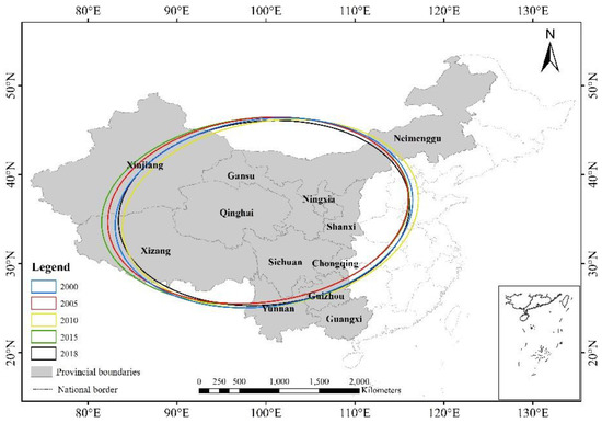
Figure 6.
Spatial distribution pattern and center of gravity transfer of annual average vegetation cover in West China.
From the coordinates of the center point in Table 3, it can be seen that the average annual centers of gravity of the western vegetation were all located in Qinghai Province. Figure 6 shows the transfer of the total spatial distribution pattern of standard deviation ellipse (SDE) center point [46,47]. The sampling points were evenly distributed in the western provinces, and the areas covered by ellipses included western Inner Mongolia, eastern Xinjiang, northeastern Tibet, northern Yunnan, northern Guizhou, Sichuan, Gansu, Chongqing, Qinghai, Ningxia, and Shaanxi. With the change of time, due to the difference of vegetation growth status, the center of gravity of vegetation in the growth period of west China has shifted and the angle of change has varied (Table 3), making the spatial distribution of standard deviation ellipse present a “northeast-southwest” pattern. The shape index in 2010 was 0.642, which shows that the shape of the main area where the spatial distribution of vegetation coverage was located in the vegetation growth season in west China in 2010 was relatively close to the standard circle.
Table 3.
Standard deviation ellipse parameters of annual average vegetation coverage in west China.
Let analysis and discussion refer to the transfer direction of the above ellipse: from 2000 to 2005, the standard deviation ellipse shifted westward, which was consistent with the aggregation type of LISA cluster diagram, indicating that under the natural and artificial influence, vegetation degradation appeared [48]; from 2005 to 2010, the standard deviation ellipse shifted eastward, which was consistent with the spatial autocorrelation distribution of vegetation coverage, indicating that vegetation growth was improved by human and self-repairing measures by 2010; from 2010 to 2015, the standard deviation ellipse shifted to the west, and from 2015 to 2018, the standard deviation ellipse shifted to the east. The directions of the ellipses in 2015 and 2018 were the same, and the center of gravity of the ellipse shifted eastward in 2018, which indicates that the vegetation growth had improved on the basis of the spatial aggregation region in 2015. The standard deviation ellipses in 2000 and 2018 partially overlapped and shifted to the east, which indicates that the vegetation coverage in these two years was relatively good and the vegetation growth was relatively consistent, It is proved that compared with the standard deviation ellipse method, which is used to research in meteorological station and economics, etc. [49,50]. In this study, it is of great significance to study the spatial change of vegetation cover, as it makes the results more intuitive and concrete.
4. Conclusions
(1) From the perspective of the spatial pattern of vegetation coverage in the growing season in west China, the proportion of NDVI and the distribution area of vegetation were analyzed and discussed. The areas with significant degradation distribution included the west adjacent to the east of Inner Mongolia, the northwest of Tibet, the northwest of Qinghai Province, a small number of areas in the east and north of Xinjiang, central Ningxia, the northwest of Gansu Province, while the areas with good vegetation coverage and significant improvement were Yunnan, Guizhou, Sichuan, Chongqing, Guangxi, the southeast of Gansu, the north of Ningxia, and the east of Inner Mongolia.
(2) According to the analysis of vegetation change trend in growing season in west China and NDVI change trend, from 2000 to 2018, the area with improved surface vegetation coverage was larger than the area with obvious vegetation degradation. The improved area accounted for 29.46% of the vegetation coverage area, the significantly degraded area accounted for 4.63%, and 65.91% of the areas were degraded and relatively stable.
(3) From the analysis of spatial autocorrelation changes of vegetation in the growing season in west China, the global spatial autocorrelation analysis shows that the vegetation coverage was lower in 2000, but the vegetation coverage increased with the passage of time, the vegetation growth status ameliorated, and its internal variation was relatively small. The autocorrelation analysis of local aggregation space shows that the vegetation coverage levels in the western, southwestern and northwestern provinces were quite different. Among them, the western regions such as Xinjiang, Gansu, Qinghai and Tibet were characterized by L-L aggregation; the southwest regions such as Sichuan, Chongqing, Guizhou, Yunnan, and Guangxi showed H-H aggregation characteristics; the northern Inner Mongolia region remained an insignificant type for 5 years.
(4) Based on the analysis of the spatial pattern change of the standard deviation ellipse of vegetation in the growing season in west China, the shift of center of gravity, direction, and angle of the standard deviation ellipse showed that the vegetation growth has improved on the basis of the spatial aggregation region in 2015. The standard deviation ellipses in 2000 and 2018 partially overlapped and shifted to the east, which indicates that the vegetation coverage in these two years was relatively good and the vegetation growth was relatively consistent.
(5) In future studies, the spatio-temporal differentiation of the driving mechanism and factors will be analyzed [51,52]. It is of significance for vegetation restoration and protection and vegetation restoration in West China.
Author Contributions
Z.B. proposed the Project Support for this study; J.Y. designed the model processing the data and wrote the paper; Q.Y., Z.G. and H.Y. polished the article. All authors have read and agreed to the published version of the manuscript.
Funding
The Key Project funded this research with the joint Fund of the National Natural Science Foundation of China, “The coal resources of Protective exploitation and environmental effects in Xinjiang” (Grant No. U1903209).
Acknowledgments
The authors gratefully acknowledge the editors and anonymous referees for their comments regarding this study. We are grateful for support from The Key Project funded this research with the joint Fund of the National Natural Science Foundation of China.
Conflicts of Interest
The authors declare no conflict of interest.
References
- Mustafa, K.; Hirable, S. Impact of Land Use Patterns on Land Degradation in the Northern Part of Sharg Al-Nile; UOFK: Khartoum, State Sudan, 2009. [Google Scholar]
- Chitade, A.Z.; Katyar, S.K. Impact analysis of open cast coal mines on land use /Land cover using remote sensing and GIS technique: A case study. Int. J. Eng. Sci. Technol. 2010, 2, 7171–7176. [Google Scholar]
- Bao, N.; Ye, B.; Bai, Z. Monitoring land degradation and reclamation change from ATB open-pit coal mine during 1976–2009. In Proceedings of the International Conference on Mechanic Automation and Control Engineering, Wuhan, China, 26–28 June 2010; pp. 1480–1485. [Google Scholar]
- Ding, W.R. Temporal and spatial Evolution characteristics of vegetation NDVI and its Driving Factors in Karst Area of Southeast Yunnan, China. Res. Soil Water Conserv. 2016, 23, 227–231. [Google Scholar]
- Liu, Y.; Fu, B.J. Topographical variation of vegetation cover evolution and the impact of land use/cover change in the Loess Plateau. Arid Land Geogr. 2013, 36, 1097–1102. [Google Scholar]
- Ma, M.G.; Wang, J.; Wang, X.M. Advance in the Inter-annual Variability of vegetation and Its Relation to Climate Base d on Remote Sensing. J. Remote Sens. 2006, 10, 421–431. [Google Scholar]
- Li, H.Y. A Dynamic study on Land degradation in Jilin province supported by RS–GIS–GPS Technique. Ji Lin Univ. 2007. (In Chinese) [Google Scholar]
- Laskin, D.; Montaghi, A.; Nielsen, S. Estimating Understory Temperatures Using MODIS LST in Mixed Cordilleran Forests. Remote Sens. 2016, 8, 658. [Google Scholar] [CrossRef]
- Kabir, A.; Kumar, G.S. Spatio-temporal Change of Vegetation NDVI and Its Relations with Regional Climate in Northern Shaanxi Province in 2000–2010. Sci. Geogr. Sin. 2014, 34, 882–888. [Google Scholar]
- Badreldin, N.; Frankl, A.; Goossens, R. Assessing the spatiotemporal dynamics of vegetation cover as an indicator of desertification in Egypt using multi-temporal MODIS satellite images. Arab. J. Geosci. 2014, 7, 4461–4475. [Google Scholar] [CrossRef]
- Liu, D.W.; Qiao, Z.Y.; Wei, T.T. The Coupling Relationship between Forest Vegetation and Terrain of Daliuta Mine. Appl. Mech. Mater. 2014, 641, 1191–1194. [Google Scholar] [CrossRef]
- Bivand, R. Spatial Data Analysis: Theory and Practice. By Robert Haining (Cambridge: Cambridge University Press, 2003). [Pp. xx + 432]. ISBN 0-521-77437-3. Price £29.95 Paperback. ISBN 0-521-77319-9. Price £80. Hardback. Int. J. Geogr. Inf. Sci. 2004, 18, 300–301. [Google Scholar] [CrossRef]
- Siderov, K. Spatial Data Analysis: Theory and Practice. Austral. Ecol. 2010, 30, 240–241. [Google Scholar] [CrossRef]
- Bian, Z.F.; Lei, S.G.; Liu, H.; Deng, K.Z. The process and countermeasures for ecological damage and restoration in coal mining area with super-size mining face at aeolian sandy site. J. Min. Saf. Eng. 2016, 33, 305–310. (In Chinese) [Google Scholar]
- Yu, F.; Price, K.P.; Ellis, J. Response of seasonal vegetation development to climatic variations in eastern central Asia. Remote Sens. Environ. 2003, 87, 42–54. [Google Scholar] [CrossRef]
- Weiss, J.L.; Gutzler, D.S.; Conrad, J.E. Long-term vegetation monitoring with NDVI in a diverse semi-arid setting, central New Mexico, USA. J. Arid Environ. 2004, 58, 249–272. [Google Scholar] [CrossRef]
- Zhang, J.; Yan, P.J. Analysis on NDVI variation characteristics of different vegetation types in shaanxi from 1982 to 2013. J. Arid Land Resour. Environ. 2017, 31, 86–92. [Google Scholar]
- Gitelson, A.A.; Kaufman, Y.J.; Stark, R. Novel algorithms for remote estimation of vegetation fraction. Remote Sens. Environ. 2002, 8, 76–87. [Google Scholar] [CrossRef]
- Gutman, G.; Ignatov, A. The derivation of the green vegetation fraction from NOAA/AVHRR data for use in numerical weather prediction models. Remote Sens. 1998, 8, 1533–1543. [Google Scholar] [CrossRef]
- Song, K.; Wang, Z.; Du, J. Wetland degradation: Its driving forces and environmental impacts in the Sanjiang Plain, China. Environ. Manag. 2014, 54, 255–271. [Google Scholar] [CrossRef]
- Nahuelhual, L.; Carmona, A.; Aguayo, M. Land use change and ecosystem services provision: A case study of recreation and ecotourism opportunities in southern Chile. Landscape Ecol. 2014, 29, 329–344. [Google Scholar] [CrossRef]
- The Statistical Bulletins of National Economic and Social Development in China 2011, National Bureau of Statistics. Available online: http://www.stats.gov.cn/statsinfo/auto2074/201310/t20131031_450700.html (accessed on 7 March 2020).
- The Statistical Bulletins of National Economic and Social Development in China 2006, National Bureau of Statistics. Available online: http://www.stats.gov.cn/tjsj/tjgb/ndtjgb/qgndtjgb/200702/t20070228_30021.html (accessed on 7 March 2020).
- Holben, B. Characteristics of maximum-value composite images from temporal AVHRR data. Int. J. Remote Sens. 1986, 7, 1417–1434. [Google Scholar] [CrossRef]
- Yu, L.; Liu, T.; Bisi, O. Trend Analysis of Maximum Hydrologic Drought Variables Using Mann–Kendall and Şen’s Innovative Trend Method. River Res. Appl. 2016, 33, 597–610. [Google Scholar]
- Shadmani, M.; Marofi, S.; Roknian, M. Trend Analysis in Reference Evapotranspiration Using Mann-Kendall and Spearman’s Rho Tests in Arid Regions of Iran. Water Resour. Manag. 2012, 26, 211–224. [Google Scholar] [CrossRef]
- Hou, J.; Du, L.T.; Ma, J.; Zhang, X.J. A study on vegetation coverage in Ning xia Autonomous region During past 20 Years based on Remote sensing and dimidiate pixel model. Bull. Soil Water Conserv. 2015, 35, 127–132. [Google Scholar]
- Noszczyk, T.; Rutkowska, A.; Hernik, J. Exploring the land use changes in Eastern Poland: Statistics-based modeling. Hum. Ecol. Risk Assess. Int. J. 2019, 1–28. [Google Scholar] [CrossRef]
- Syed, S.S.; Imran, A.S. Spatial pattern analysis of seeds of an arable soil seed bank and its relationship with above-ground vegetation in an arid region. J. Arid Environ. 2004, 3, 311–327. [Google Scholar]
- Diouf, A.; Lambin, E.F. Monitoring land-cover changes in semi-arid regions: Remote sensing data and field observations in the Ferlo, Senegal. J. Arid Environ. 2001, 48, 129–148. [Google Scholar] [CrossRef]
- Jian, P.; You, L.; Lu, T. Vegetation Dynamics and Associated Driving Forces in Eastern China during 1999–2008. Remote Sens. 2015, 7, 13641–13663. [Google Scholar]
- Jiang, W.G.; Yuan, L.H.; Wang, W.J. Spatio-temporal analysis of vegetation variation in the Yellow River Basin. Ecol. Indic. 2014, 51, 117–126. [Google Scholar] [CrossRef]
- Eryando, T.; Susanna, D.; Pratiwi, D. Standard Deviational Ellipse (SDE) models for malaria surveillance, case study: Sukabumi district-Indonesia, in 2012. Malar. J. 2012, 11, P130. [Google Scholar] [CrossRef]
- Karlsen, S.; Elvebakk, A.; Hgda, K. Spatial and Temporal Variability in the Onset of the Growing Season onSvalbard, Arctic Norway—Measured by, MODIS-NDVI Satellite Data. Remote Sens. 2014, 6, 8088–8106. [Google Scholar] [CrossRef]
- Machida, F.; Andrzejak, A.; Matias, R. On the effectiveness of Mann-Kendall test for detection of software aging. In Proceedings of the 2013 IEEE International Symposium on Software Reliability Engineering Workshops (ISSREW), Pasadena, CA, USA, 4–7 November 2013. [Google Scholar]
- Walter, D.K. Spatial autocorrelation of ecological phenomena. Trends Ecol. Evol. 1999, 14, 22–26. [Google Scholar]
- Nobuhiko, T.; Masayoshi, K. The Size-adjusted Critical Region of Moran’s I Test Statistics for Spatial Autocorrelation and Its Application to Geographical Areas. Geogr. Anal. 1994, 3, 213–227. [Google Scholar]
- Karan, S.K.; Samadder, S.R.; Maiti, S.K. Assessment of the capability of remote sensing and GIS techniques for monitoring reclamation success in coal mine degraded lands. J. Environ. Manag. 2016, 182, 272–283. [Google Scholar] [CrossRef] [PubMed]
- Tripathy, G.K.; Ghosh, T.K.; Shah, S.D. Monitoring of desertification process in Karnataka state of India using multi-temporal remote sensing and ancillary information using GIS. Int. J. Remote Sens. 1996, 17, 2243–2257. [Google Scholar] [CrossRef]
- Deng, K.L.; Fan, J.Z.; Quan, W.T. Analysis of vegetation degradation and its driving factors in Shaanxi Province. Chin. J. Ecol. 2015, 20, 680–683. (In Chinese) [Google Scholar]
- Liu, Y.; Wang, Y.; Jian, P. Correlations between Urbanization and Vegetation Degradation across the World’s Metropolises Using DMSP/OLS Nighttime Light Data. Remote Sens. 2015, 7, 2067–2088. [Google Scholar] [CrossRef]
- Diallo, H.A. United Nations Convention to Combat Desertification (UNCCD). In The Future of Drylands; Springer: Dordrecht, The Netherlands, 2008; pp. 13–16. [Google Scholar]
- Sheng, Y.; Wang, C.Y. Applicability of Prewhitening to Eliminate the Influence of Serial Correlation on the Mann-Kendall Test. Water Resour. Res. 2002, 6, 1–4. [Google Scholar]
- Bian, Z.F.; Shen, W.S. Driving Factors of Land Degradation in Major Mining Areas in West China. J. Ecol. Rural Environ. 2016, 32, 173–177. (In Chinese) [Google Scholar]
- Gong, J. Clarifying the standard deviational ellipse. Geogr. Anal. 2002, 34, 155–167. [Google Scholar] [CrossRef]
- Yuill, R.S. The Standard Deviational Ellipse; An Updated Tool for Spatial Description. Geogr. Ann. Ser. B Hum. Geogr. 1971, 53, 28–39. [Google Scholar] [CrossRef]
- Kousari, M.R.; Ahani, H.; Hendi, R. Temporal and spatial trend detection of maximum air temperature in Iran during 1960–2005. Glob. Planet. Chang. 2013, 111, 97–110. [Google Scholar] [CrossRef]
- Li, S.T.; Yang, M.L.; Li, L. Evaluation on Data Quality of X-band Dual Polarization Weather Radar Based on Standard Deviation Analysis. J. Arid Meteorol. 2019, 37, 467. [Google Scholar]
- Wu, S.H.; Gao, J.B.; Deng, H.Y. Climate change risk and its quantitative assessment methods. Prog. Geogr. 2018, 37, 28–35. (In Chinese) [Google Scholar]
- Biancalani, R.; Nachtergaele, F.O.; Petri, M. Land Degradation Assessment in Drylands—Methodology and results. 2011 and human factors to desertification in northwest China using net primary productivity as an indicator. Ecol. Indic. 2015, 48, 560–569. [Google Scholar]
- Shen, Y.; Liao, X.; Yin, R. Measuring the Aggregate Socioeconomic Impacts of China’s Natural Forest Protection Program. In An Integrated Assessment of China’s Ecological Restoration Programs; Springer: Dordrecht, The Netherlands, 2009; Volume 07, pp. 235–254. [Google Scholar]
- Li, Z.J.; Tang, Y.N. Research on the Torpedo Sinker of Ellipse-like Body of Streamline and its Standardization and Systematization. J. Chang. Vocat. Univ. 2000, 04, 29–32. [Google Scholar]
© 2020 by the authors. Licensee MDPI, Basel, Switzerland. This article is an open access article distributed under the terms and conditions of the Creative Commons Attribution (CC BY) license (http://creativecommons.org/licenses/by/4.0/).