Abstract
Over the last 15 years, the Gravity Recovery and Climate Experiment (GRACE) mission has provided measurements of temporal changes in mass redistribution at and within the Earth that affect polar motion. The newest generation of GRACE temporal models, are evaluated by conversion into the equatorial components of hydrological polar motion excitation and compared with the residuals of observed polar motion excitation derived from geodetic measurements of the pole coordinates. We analyze temporal variations of hydrological excitation series and decompose them into linear trends and seasonal and non-seasonal changes, with a particular focus on the spectral bands with periods of 1000–3000, 450–1000, 100–450, and 60–100 days. Hydrological and reduced geodetic excitation series are also analyzed in four separated time periods which are characterized by different accuracy of GRACE measurements. The level of agreement between hydrological and reduced geodetic excitation depends on the frequency band considered and is highest for interannual changes with periods of 1000–3000 days. We find that the CSR RL06, ITSG 2018 and CNES RL04 GRACE solutions provide the best agreement with reduced geodetic excitation for most of the oscillations investigated.
1. Introduction
Polar motion (PM) is affected by a wide range of processes with different temporal variability ranging from several days to many decades [1]. Such disturbances include the gravitational influence of other celestial bodies, continuously changing mass distribution in the Earth’s surficial fluids (atmosphere, oceans and land hydrosphere), the effects of core–mantle coupling, and also groundwater depletion and ice mass loss resulting from recent climate changes [2,3,4].
It is commonly known that for time scales of a few years or less, the main contributors to variation in Earth’s rotation are angular momentum changes of the solid Earth caused by mass redistribution in the Earth’s surficial fluids. The excitation of polar motion due to changes in mass redistribution of atmosphere, ocean and land hydrosphere can be represented with effective angular momentum (EAM) functions: atmospheric, oceanic and hydrological. Information about mass transport in the Earth’s fluid layers can be obtained from observations of temporal changes of the gravity field. Such measurements were provided from 2002 to 2017 by the Gravity Recovery and Climate Experiment (GRACE) mission [5]. The variations of degree-2, order-1 Stokes coefficients (ΔC21, ΔS21) of geopotential are commonly used in determination of mass-related PM excitation since they are proportional to the χ1 and χ2 components of the PM excitation [6]. The leading GRACE data centres at GeoForschungsZentrum (GFZ) in Potsdam, Germany; Center for Space Research (CSR) in Austin, USA; and the Jet Propulsion Laboratory (JPL) in Pasadena, USA, provide monthly GRACE gravity solutions in the form of Stokes coefficients (also named GRACE Level-2 data or GRACE satellite-only model (GSM) coefficients). Recently, new GRACE solutions (Release 6 or RL06) have been developed and made available to the scientific community by GFZ, CSR, and JPL. However, during the 15 years of the mission, new centers also joined the network. Thus, the Institute of Theoretical Geodesy and Satellite Geodesy (ITSG) of the Graz University of Technology, Austria, and the Groupe de Recherche en Géodésie Spatiale (GRGS)/Centre National d’Etudes Spatiales (CNES) in Toulouse, France, have also developed their own new solutions, known as ITSG-Grace2018 (abbreviated here as ITSG 2018) and CNES/GRGS RL04 (abbreviated here as CNES RL04), respectively.
The role of atmospheric and oceanic mass distribution on the global balance of Earth’s angular momentum, described as atmospheric and oceanic angular momentum (AAM and OAM, respectively), is well established [7,8,9,10,11,12,13]. However, the role of the continental hydrosphere, referred to as hydrological angular momentum (HAM) or the hydrological excitation, is less clear as indications from different hydrological models do not agree well with each other [14,15,16,17,18]. Moreover, other geophysical effects, such as the consequences of co- and post-seismic deformations associated with large earthquakes [19], and the coupling between the Earth’s core and the lower mantle [20,21], are often not considered in a rigorous way.
The GRACE observations of changing Earth’s mass redistribution improve the understanding of the signals in polar motion (PM) excitation caused by time-variations in the Earth’s mass distribution. After removing tidal effects (atmospheric, ocean, solid Earth, and pole tides), as well as non-tidal atmospheric and oceanic contributions from the GRACE-based geopotential coefficients, the remaining signal is mostly an indication of the land hydrosphere [22], glacial isostatic adjustment (GIA) [23], barystatic sea-level contributions [24], and earthquake signatures [25]. GRACE-based PM excitation has been assessed before [8,12,15,16,26,27,28,29,30], but considerable differences were found among the processing centers.
The newly processed GRACE RL06 solutions benefit from a thorough reprocessing of the Level-1 sensor data, in particular the star tracker data and the K-band range-rate observations. Improvements were also the results of using a re-processed Global Positioning System (GPS) constellation, from refined data screening procedures that lead to a reduced number of apparently detected outliers, and from the revision of various parametrization schemes of both the accelerometers and the K-band ranging [31,32,33]. Moreover, various background models have been updated for RL06, including a new mean pole model (linear instead of cubic; [34]), the new GRACE Atmosphere and Ocean De-Aliasing Level-1B RL06 (AOD1B RL06; [35,36]) product, improved ocean tides models and static gravity field models, and updated planetary ephemerides for perturbations induced by the large planets of the solar system [31,32,33].
The objective of this study is to evaluate what the new GRACE RL06 solutions might contribute to the understanding of residual PM excitations as observed by space geodetic techniques. An early comparison of PM excitations from the new GRACE RL06 solutions with the estimates from a previous release (RL05) have already been published [37]. Those authors underlined unprecedented improvement of mass-related PM excitation obtained from newly-processed GRACE data, and an increase of consistency between solutions from different processing centers. They also showed that the update mostly influenced oceanic and hydrological excitation. We provide here a complementary analysis of linear trends and seasonal and non-seasonal oscillations, and a number of specifically selected spectral bands. In addition, we conducted our analyses for four different time periods which were characterized by different accuracy of GRACE measurements. For quantitative analyses we compared correlation coefficients with observed PM excitation, relative explained variance, and standard deviation of the series. We also analyzed phasor diagrams of seasonal changes, namely annual, semi-annual, and ter-annual. The study aimed to identify the solutions that best match geodetic observations of PM in specific spectral bands, which can be recommended for use in further analyses focusing on certain oscillations.
2. Data and Methodology
2.1. Hydrological Signals in Observed Polar Motion—Geodetic Residuals
Observed or geodetic polar motion excitation (geodetic angular momentum, GAM) can be obtained from observed coordinates (x, y) of the pole by solving Liouville’s equation [38,39]. In this research, the equatorial components (χ1 and χ2) of GAM are computed from x, y, which are taken from the daily combined 14 C04 series of Earth Orientation Parameters (EOP) derived from GNSS (Global Navigation Satellite Systems), SLR (Satellite Laser Ranging), and VLBI (Very Long Baseline Interferometry). EOP 14 C04 series are fully consistent with the International Terrestrial Reference Frame 2014 (ITRF 2014) [40,41]. The EOP data are provided by the International Earth Rotation and Reference System Service (IERS) (https://www.iers.org/IERS/EN/DataProducts/EarthOrientationData/eop.html) and updated on a regular basis with typically 30 days latency. In this study, for computation of GAM, we used an algorithm given at http://hpiers.obspm.fr/eop-pc/index.php?index=excitactive&lang=en.
Observed GAM are commonly reduced for the effects of atmosphere and ocean to study only the residual signals, denoted as geodetic residuals (GAM − AAM − OAM or GAO), using the following method:
where GAM, AAM and OAM are geodetic angular momentum, atmospheric angular momentum and oceanic angular momentum, respectively. Note that here, AAM and OAM are effective angular momentum functions of atmosphere and ocean, which are sometimes abbreviated as EAM or EAMF of atmosphere and ocean.
GAO = GAM − AAM − OAM,
The resulting series are expected to represent the impact of land hydrosphere and barystatic sea-level changes on PM excitation. Nevertheless, it should be kept in mind that GAO will also contain signals from changes in the mass of ice sheets, the effects of large earthquakes [42,43], and the signatures of geomagnetic jerks [44].
The following data sets were used for this study to calculate GAO:
- χ1 and χ2 equatorial components of GAM: obtained from the IERS website (https://www.iers.org/IERS/EN/Home/home_node.html), with temporal resolution of 24 h;
- χ1 and χ2 equatorial components of the AAM: provided by the GFZ, and based on ECMWF (European Center for Medium-Range Weather Forecasts) model [45]. The series are available at temporal resolution of 3 h and can be accessed from http://rz-vm115.gfz-potsdam.de:8080/repository (Earth System Model GFZ (ESMGFZ) data). Note that the current AAM version provided by GFZ is consistent with GRACE AOD1B RL06 Atmosphere and Ocean De-Aliasing Level-1B Release-6 (AOD1B RL06) [35,36];
- χ1 and χ2 equatorial components of the OAM: provided by the GFZ, and based on MPIOM (Max Planck Institute Ocean Model) [46]. The series are available at temporal resolution of 3 h and can be accessed from http://rz-vm115.gfz-potsdam.de:8080/repository (ESMGFZ data). Note that the current OAM version provided by GFZ is consistent with GRACE AOD1B RL06.
The use of ESMGFZ data for computing GAO provides consistent results with GRACE estimations, because AOD1B RL06 and ESMGFZ were based on the same input models. Any other AAM and OAM data set would complicate the analysis by introducing unknown effects into the comparison.
It should be kept in mind that C04 EOP daily series suffer some weaknesses connected with aliasing of sub-daily signals caused by mis-modelled ocean tides. It is known that pole coordinates contain diurnal and sub-diurnal signals reaching 1 mas (miliarcsecond, 1 mas ≅ 3,09 cm on the Earth’s surface) [41]. However, these high-frequency tidal signals cannot be included in 24-h C04 EOP series dedicated to providing reference Earth orientation data on a daily time rate. Nevertheless, in our study we focus on monthly PM excitation changes, so this should not affect our results.
The C04 EOP data have recently been reprocessed to ensure consistency with the new ITRF 2014 [47] and we used these updated series. The new daily EOP combined 14 C04 series were recomputed from 1984 according to improved algorithms and replaced the previous 08 C04 series in February 2017. The main reason for this reprocessing was that the differences between the former 08 C04 series and the EOP produced jointly with the ITRF 2014, starting from 2010, produced a bias in the y pole coordinate that reached 50 μas (microarcsecond) above the mean formal uncertainty estimated by the IGS (International GNSS Service) [41]. The 14 C04 EOP has been tied to the ITRF 2014 EOP solution and IVS (International VLBI Service for Geodesy and Astrometry) combination to provide consistency with the conventional ITRF 2014 [47] and ICRF2 (Second International Celestial Reference Frame) [48] reference frames.
2.2. Polar Motion Excitation Derived from GRACE
The relationship between ΔC21, ΔS21 coefficients of the geopotential and the equatorial components of the PM excitation (χ1 and χ2) can be expressed as follows (based on [39] and Chapter 3.09.5 in [6]):
where, ΔC21 and ΔS21 are the fully normalized Stokes coefficients of the Earth’s gravity field; Re and M are the Earth’s mean Earth’s radius (6378136.6 m) and mass (5.9737 × 1024 kg), respectively; A = 8.0101 × 1037 kg∙m2, B = 8.0103 × 1037 kg∙m2, and C = 8.0365 × 1037 kg∙m2 are the Earth’s principal moments of inertia, and A′ = (A+B)/2 is the average of the equatorial Earth’s principal moments of inertia (Table 1 in [6]).
The PM excitation series obtained from the GRACE observations as represented by the monthly GRACE satellite-only models (GSM) are sometimes denoted as gravimetric–hydrological excitation, or simply as GRACE-based HAM. As indicated above, we note that the Level-2 monthly-mean gravity fields from GRACE contain not only the mass effects from terrestrial water storage, but also other signals such as the barystatic sea-level changes due to inflow of continental water into the oceans, GIA effects, or tectonic signals related to large earthquakes. We thus denoted the GRACE-based angular momentum series as GSMAM to emphasize that they were derived from the Level-2 GSM fields of GRACE. During the processing of GRACE data, the signals from short-term non-tidal atmospheric and oceanic variations were reduced by applying AOD1B [35,36]. Therefore, GSMAM series do not contain these effects.
In this study, we compared the following monthly times series of time-variable Level-2 GRACE GSM fields provided by five different processing groups:
- CSR, Austin, USA—CSR RL06 [31] solution,
- JPL, Pasadena, USA—JPL RL06 [33] solution,
- GFZ, Potsdam, Germany—GFZ RL06 [32,49] solution,
- ITSG, Graz University of Technology, Austria—ITSG-Grace2018 (called further ITSG 2018) [50] solution,
- CNES/GRGS, Toulouse, France—CNES/GRGS RL04 (called further CNES RL04) [51] solution.
The time series were accessed from the International Center for Global Earth Models (ICGEM) website (http://icgem.gfz-potsdam.de/home), JPL PO.DAAC Drive (https://podaac-tools.jpl.nasa.gov/drive/files/GeodeticsGravity/grace/L2), and CNES/GRGS website (http://grgs.obs-mip.fr/grace). Available GRACE series have quasi-monthly time resolution and cover the time period between April 2002 and May 2017 (for CSR RL06, JPL RL06, GFZ RL06 and ITSG 2018), and between September 2002 and June 2016 (for CNES RL04). Detailed information about considered solutions, with background models and data sources are given in Table A1 in Appendix A. Table A1 also contains corresponding information for previous GRACE RL05 solutions.
It should be noted that the CNES RL04 and ITSG 2018 solutions were designed to be compatible with official CSR RL06, JPL RL06 and GFZ RL06 data and were published around the same time, so, we used the RL06 indication for all five solutions throughout the remainder of this paper.
Regarding to the series from GFZ, it is now officially recommended to replace C21/S21 coefficients for GFZ RL06 with SLR estimates [49]. These coefficients are estimated from a GRACE and SLR combination on the level of normal equations. Each monthly estimate is fully independent from the rest of the time series. Additionally, C20 and C30 coefficients need to be replaced according to this recommendation, but in this work we focus only on GSMAM computed from C21, S21. In the current study, for GFZ estimates, we consider GSMAM obtained from both the non-combined GFZ RL06 solution and the combined GFZ RL06 + SLR series. The latter are denoted in this paper as the GRACE + SLR series.
2.3. HAM and SLAM Processed by GFZ
We also considered HAM based on the Land Surface Discharge Model (LSDM) and accessed from GFZ (ftp://esmdata.gfz-potsdam.de/EAM). The LSDM simulates both vertical and lateral water transport and storage on land surfaces [52,53]. It is given in a regular 0.5° × 0.5° global latitude–longitude grid and with a 24 h time step. LSDM is forced with precipitation, evaporation, and surface temperature from the ECMWF model. The χ1, χ2 LSDM-based HAM excitation series were taken directly from the GFZ website.
It should be remembered that while comparing HAM obtained from hydrological models with GSMAM derived from GRACE data, it is crucial to add the contribution of barystatic sea level changes due to inflow of water from lands into the oceans (sea-level angular momentum, SLAM) to model-based HAM. It is important, because both GRACE GSM fields and GAM (and also GAO which was computed after removing AAM and OAM from GAM) include SLAM, but it is not modeled in hydrological models. Therefore, in this study, we added SLAM to LSDM-based HAM. The SLAM series were based on ECMWF and LSDM data, provided by the GFZ (ftp://esmdata.gfz-potsdam.de/EAM) and available in the form of χ1, χ2 [54].
Our motivation for choosing HAM from GFZ was that the consistent SLAM part of the excitation is publicly available only for the GFZ data set. This SLAM series are also compatible with GRACE AOD1B dealiasing data. To show how large the error would be if mass balance was not considered, we can give the relation of SLAM/(HAM + SLAM). The most preferred value of this dimensionless ratio is 1 (which means that SLAM and HAM + SLAM are the same). For the time period considered here, this value ranges from −9.0 to +3.7 for χ1 and from −10.3 to +3.0 for χ2, with standard deviations of 1.4 and 1.3 for χ1 and χ2, respectively. The variability of SLAM is smaller than variability of HAM + SLAM as standard deviation of SLAM series represents 28% of standard deviation of HAM + SLAM for χ1 and 19% for χ2. Another motivation to choose HAM based on LSDM were our previous results [15], which showed that compared to other hydrological and climate models, LSDM provided higher consistency with GAO and GRACE-based excitation series. In this study, we consider only the sum of HAM and SLAM, using the term HAM + SLAM throughout the remainder of this paper.
3. Results
In this paper, we focus on the overall analysis of month-to-month variations in time series (Section 3.1), month-to-month variations and trends in time series for four time periods characterized by different accuracy of GRACE observations (Section 3.2), secular trends, seasonal and non-seasonal oscillations (Section 3.3), and variations in four different frequency bands with periods of 60–100, 100–450, 450–1000, and 1000–3000 days (Section 3.4).
3.1. Overall Comparison of GSMAM Series
Initially, we display time series of GSMAM computed using different GRACE solutions and GRACE + SLR, without applying any filtering (Figure 1a,b). The series have quite similar character with strong positive trends in χ1, weaker negative trends in χ2, visible annual variation, and some other oscillations of periods both shorter and longer than annual. It is obvious that GRACE + SLR series are less noisy than GSMAM from GFZ RL06 solution. Notably, after 2016, the series became more noisy, as the accuracy of GRACE decreased due to a change in thermal control of the spacecraft due to the increasingly limited battery capacity. In 2017, one accelerometer was turned off and that caused a further degradation of the results, especially visible for GFZ and ITSG solutions. Figure 1 gives also formal errors of estimated χ1, χ2, which were computed from the errors of ΔC21, ΔS21 coefficients (Figure 1c–f) (errors for CNES RL04 were not available). It is visible that the best GRACE performance occurs in the years 2006–2013, and before and after this period the error values are higher and noisier. During the entire 15-year GRACE operational period, some peaks of visibly higher errors occurs typically related to occasional periods of short repeat orbits. Compared to other GRACE solutions, the CSR RL06 series has the lowest and the most stable errors of χ1 and χ2. However, the errors of GRACE + SLR series are even lower. Notably, after 2005, the errors of GFZ-based excitation series start to increase almost linearly.
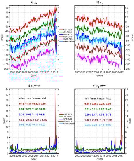
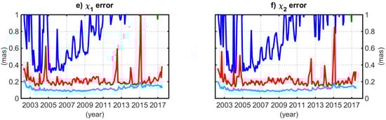
Figure 1.
χ1 (a) and χ2 (b) components of GSMAM computed using ΔC21, ΔS21 from different Gravity Recovery and Climate Experiment (GRACE) solutions and from GRACE + SLR and their standard errors (c,d). Plots of errors (c,d) were supplemented with the values of minimum, maximum, mean and standard deviation (STD) of errors. No filtering and no interpolation have been applied to the series. For better visibility, χ1 (a) and χ2 (b) time series have been shifted relative to each other by adding a bias; (e) and (f) show the same as (c) and (d) but with changed scale for y axis to show variability of GRACE + SLR errors.
Due to some gaps in the GRACE observations, different temporal sampling intervals (3 h for ECMWF and MPIOM models, 24 h for GAM, HAM from LSDM and SLAM, and only monthly for GRACE), and different periods in which these data are available, all time series were downsampled to monthly time-steps, using a Gaussian filter with full width at half maximum (FWHM) parameter of 60 days. In the reminder of this paper, we considered the same period for all data sets, namely between September 2002 and June 2016, except for the tests reported in Section 3.2.
Figure 2 presents time series of χ1, χ2 components of hydrological PM excitation obtained from all considered GSMAM solutions as well as GRACE + SLR and GFZ HAM + SLAM, together with the GAO. To assess the variability of time series, we also computed their standard deviation (Table 1). In general, the new RL06 GRACE solutions underestimate the standard deviation of GAO particularly for χ2. In order to quantify the agreement between GAO and different GSMAM, we computed correlation coefficients and relative explained variance between evaluated and reference series (Table 1). The relative explained variance (Varexp) describes the variability agreement between two time series, reference series (r) and evaluated series (e):
where Var(r), Var(e) and Var(r−e) are variance of reference series, variance of evaluated series and variance of a difference between the reference and evaluated series, respectively. In this study, the reference series are GAO and the evaluated series are GSMAM, GRACE + SLR and HAM + SLAM. There is a better consistency of GSMAM series with GAO for the case of χ2 component, which has been already reported in previous research (e.g., [7,12,15,16,17,30,55]), and is tightly related to the continent-ocean distribution. The values given in Table 1 reveal that CSR RL06, ITSG 2018 and CNES RL04 solutions provide the highest correlation coefficients with GAO and the most satisfactory relative explained variance values for both χ1 and χ2. Notably, HAM + SLAM obtained from models processed by GFZ, exhibits results comparable with those from CSR RL06, ITSG 2018 and CNES RL04, but only in χ2. GRACE + SLR series are highly more consistent with GAO than GFZ-based GSMAM, however, the results are not as satisfactory as for GSMAM from CSR RL06 data.
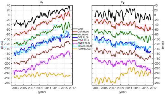
Figure 2.
χ1 and χ2 components of GAO, GSMAM, GRACE + SLR and HAM + SLAM obtained from geophysical models processed at GFZ. Each time series was filtered using Gaussian filter with FWHM (full width at half maximum) equal to 60 days. The same time period was considered for all data sets, namely between September 2002 and June 2016.

Table 1.
Standard deviation of time series, correlation coefficients with GAO, and percentage of variance in GAO explained by GSMAM, GRACE + SLR and HAM + SLAM. Before computing the values, linear trends were removed from the series. Note that the critical value of the correlation coefficient for 54 independent points and the confidence level of 0.95 was 0.23. The standard error of the difference between two correlation coefficients for 54 independent points was 0.20. The highest values of correlations and relative explained variances are italicized.
In general, polar motion excitation shows two circular motions with opposite directions: clockwise, usually called retrograde, with frequency marked as negative, and counter-clockwise, named prograde, with frequency marked as positive [7,56,57]. It is common in the study of polar motion that the seasonal elliptical wave is represented as a combination of prograde and retrograde circular motions, rather than the equatorial χ1 and χ2 components related to the Earth-fixed system. This method of presentation facilitates the physical interpretation of seasonal PM excitation because the transfer function between the polar motion and polar excitation function is asymmetrical with respect to zero frequency. Such prograde and retrograde seasonal variations in PM excitation are usually represented by amplitudes and phases of annual, semi-annual and ter-annual oscillations [7,8,16,17,18,30,45]. However, it is also possible to determine prograde and retrograde terms of PM excitation without focusing on specific frequency [56,57].
It is known that seasonal oscillation is the strongest signal in hydrological excitation of PM but it is possible to check the magnitude of other spectral bands by plotting amplitude spectra of the complex-valued components of χ1 + iχ2. To check the oscillation amplitude distribution in GSMAM, GAO, GRACE + SLR and HAM + SLAM, we present such kind of spectra for all considered excitation series in Figure 3. The spectra are computed using a Fourier Transform Band Pass Filter (FTBPF) [58] in the broadband with a 60- and 3000-day cut-off (Figure 3a) and in the broadband with 60- and 450-day cut-off (Figure 3b). It should be kept in mind that the oscillations with periods shorter than 60 days cannot be considered, because all series were monthly sampled and their Nyquist frequency is about 6 cycles per year (cpy) that corresponds to the periods of about 60 days. The spectra show that there are several amplitude peaks in a band of 60–450 days with annual signal being the strongest (Figure 3a,b). For GAO and most of GSMAM series, some longer oscillations are also visible, namely 450–1000 days in prograde band, 450–700 days in retrograde band and 1000–3000 days in both prograde and retrograde bands (Figure 3a). Figure 3b shows that the spectra of all considered series exhibit annual and semi-annual oscillations, both in the prograde and retrograde bands. The retrograde oscillations of the GAO have greater amplitudes than any of the considered GSMAM series (Figure 3a). In the prograde band, for the periods between 60 and 1000 days, GAO series is the most powerful, but for longer oscillations, GSMAM from GFZ RL06 reveals to have the highest amplitudes. The spectra obtained from HAM + SLAM has almost the weakest amplitudes for the whole prograde spectral band and also the retrograde semi-annual oscillations are the least energetic. However, HAM + SLAM captures the strong annual retrograde peak of GAO the best.
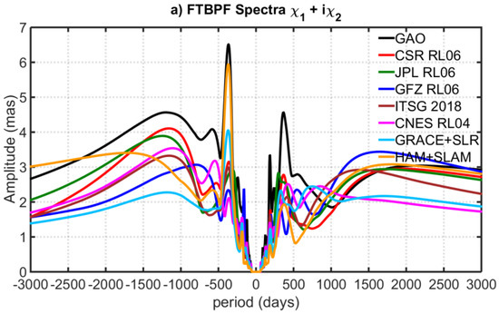
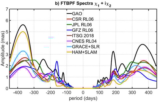
Figure 3.
Fourier Transform Band Pass Filter (FTBPF) amplitude spectra of the GAO, GSMAM, GRACE + SLR, and HAM + SLAM computed in a broadband with (a) a 60–3000 day cut-off and (b) 60–450 day cut-off. The parameter λ describing the filter bandwidth when computing the FFBPF spectra was equal to 0.018. The minus time period on the plot indicates retrograde terms while plus time period indicates prograde terms.
3.2. Analysis of GSMAM Series for Different Time Periods
As it was noticed in Section 3.1, throughout the duration of the GRACE mission, the accuracy of its observations has not been stable, and this could affect the GSMAM quality assessment (see Figure 1). Moreover, in our previous work [59] we demonstrated that the trends in GAO depended strongly on considered time period. Therefore, this section evaluates GSMAM, GRACE + SLR and HAM + SLAM in several different time periods. Based on the information about the errors of GSMAM (Figure 1), we select the following time intervals: (1) April 2002–January 2006, (2) January 2006–January 2014, (3) January 2014–January 2017, and (4) January 2017–June 2017. The tests include: trend analysis (Figure 4 and Figure 5); comparison of time series variability expressed by standard deviation (STD) (Table 2); the test of GSMAM, GRACE + SLR and HAM + SLAM compatibility with GAO, conducted using correlation coefficients (Table 3) and relative explained variances (Table 4).
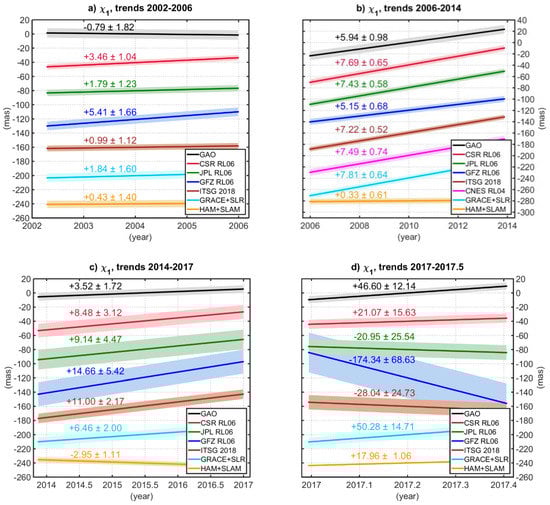
Figure 4.
Trends in χ1 component of GAO, GSMAM, GRACE + SLR, and HAM + SLAM together with their errors for four time periods: (a) 2002–2006, (b) 2006–2014, (c) 2014–2017, (d) 2017–2017.5. The values are given in mas/year. The shades show the errors of trends determined. Note that CNES RL04 data covered only the period 2006–2014 in full and was not included in (a), (c) and (d).
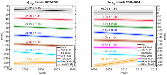
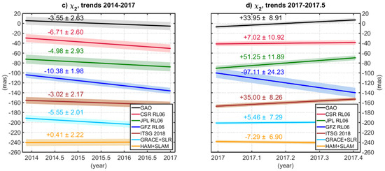
Figure 5.
Trends in χ2 component of GAO, GSMAM, GRACE + SLR, and HAM + SLAM together with their errors for four time periods: (a) 2002–2006, (b) 2006–2014, (c) 2014–2017, (d) 2017–2017.5. The values are given in mas/year. The shades show the errors of trends determined. Note that CNES RL04 data covered only the period 2006–2014 in full.
Table 2.
Standard deviation of GAO, GSMAM, GRACE + SLR, and HAM + SLAM time series for four considered time periods. Note that CNES RL04 was included only for the period 2006–2014.
Table 3.
Correlation coefficients between GAO and GSMAM, between GAO and GRACE + SLR, and between GAO and HAM + SLAM for four considered time periods. Before computing the values, linear trends were removed from the series. Note that CNES RL04 was included only for the period 2006–2014. The highest values of correlations are italicized.
Table 4.
Percentage of variance in GAO explained by variance of GSMAM, GRACE + SLR, and HAM + SLAM for four considered time periods. Before computing the values, linear trends were removed from the series. Note that CNES RL04 was included only for the period 2006–2014. The highest values of relative explained variances are italicized.
In terms of χ1, apart from 2002–2006 period, GAO is characterized by positive trend (Figure 4). As it was expected, for the period of the highest GRACE accuracy, the GSMAM trends in χ1 are very compatible with each other and with GAO trend (Figure 1b). For this period, the maximum difference between GAO trend and GSMAM trend reaches 1.75 mas/year (for CSR RL06), while the minimum difference is equal to 0.79 mas/year (for GFZ RL06). For each considered time interval, GSMAM overestimates χ1 GAO trend while HAM + SLAM underestimates it. For χ2, the GAO trend signs are less steady (Figure 5). As it can be seen from Figure 5, χ2 GSMAM trends are the most consistent with GAO trends and with each other for the initial period of the GRACE mission (2002–2006). For this time interval, the maximum difference between GAO trend and GSMAM trend reaches 1.48 mas/year (for GFZ RL06), while the minimum difference is equal to 0.46 mas/year (for CSR RL06). Notably, in the period of the lowest GRACE observations errors (2006–2014, see Figure 1c,d) GSMAM trend signs in χ2 are inconsistent with GAO trend sign (Figure 5b). We can generally conclude that the trend of HAM + SLAM series processed by GFZ is rather incompatible with trend of GAO for both χ1 and χ2. Note that trends for the period 2017 until 2017.5 are reported for completeness, but not discussed due to the limited data coverage in that period.
The values of STD of time series given in Table 2 prove that the variability of GAO, GSMAM, GRACE + SLR and HAM + SLAM depend on time period considered. For the periods of 2002–2006 and 2006–2014, GSMAM series underestimates STD of GAO, while for the last years of the GRACE mission, the variability of GSMAM is higher than variability of GAO. This can be associated with decreased accuracy and increased noise of GRACE observations after 2014 (see Figure 1c,d).
In general, the consistency between GSMAM and GAO, described by correlation coefficients (Table 3), is the highest for 2006–2014 and the lowest for 2017–2017.5. The exception are GSMAM series obtained from CSR RL06 and JPL RL06 solutions, for which we observe very high correlations with GAO during the last operational period of GRACE satellites, but only for χ2. However, only a six-month period of data cannot allow objective conclusions to be drawn. In the initial period of GRACE observations (2002–2006), the biggest consistency with GAO for both χ1 and χ2 is provided by GSMAM from CSR RL06, while JPL RL06 gives satisfactory results for χ1 only and ITSG 2018 provides high correlation for χ2 only. The period of 2006–2014 is characterized by the highest correlation agreement between GSMAM and GAO, with the best results for CSR RL06 (for both χ1 and χ2), ITSG 2018 (for both χ1 and χ2) and CNES RL04 (for χ2 only). After 2014, the correlation values start dropping and they reach their maximum for CSR RL06 (for both χ1 and χ2) and ITSG 2018 (for χ1 only) in the period of 2014–2017. After turning off the accelerometer on one of the GRACE satellites in 2017, the correlations with GAO remain positive for both χ1 and χ2 only for GSMAM from CSR RL06. This is confirmed by the lowest errors for CSR data compared to other GRACE solutions (see Figure 1c,d). It is worth mentioning that HAM + SLAM series computed from numerical models processed by GFZ provides high correlation with GAO for all considered time periods particularly for χ2. This indicates that residual error of the ocean circulation remains both in GSM and GAO that are not explained by SLAM. This means that it requires further efforts to improve in particular the oceanic non-tidal background model for both GRACE and the EOP.
The analysis of relative explained variances (Table 4) generally confirms the conclusions presented above. In particular, CSR RL06 reveals to provide the highest variance agreement with GAO for both χ1 and χ2 in 2002–2006 and 2006–2014. GSMAM from ITSG 2018 gives high variances in 2002–2006 (for χ1 only) and 2006–2014 (for both χ1 and χ2), while CNES RL04 provides satisfactory results for χ2 in 2006–2014. Notably, after 2014, the variance agreement between GSMAM and GAO visibly decreases as most values are negative. This may be due to the fact that around 2014, GRACE observations are increasingly affected by aging instruments. χ2 component appears to be less affected than χ1. Only CSR RL06 data provide positive relative explained variances for both 2014–2017 and 2017–2017.5 periods, but only in χ2. It should be mentioned that for χ2 component, HAM + SLAM series provides the highest variance agreement with GAO for all considered time periods.
3.3. Analysis of Trends and Seasonal and Non-Seasonal Oscillation
We now focus on several analyses of GAO, GSMAM, GRACE + SLR and HAM + SLAM conducted for the same period, namely between September 2002 and June 2016. The most common methods to compare PM excitation series from different data sources involve either comparing full time series [12,14,30,37,60,61,62] or decomposing them into seasonal and non-seasonal oscillations [8,15,17,18,45]. We now decompose all series into linear trends, and seasonal and non-seasonal changes. To calculate linear trends and seasonal oscillations, we use a least-squares method to fit a seasonal model to the series. The model comprises the first-degree polynomial and the sum of sinusoids with the periods of 365.25, 182.625, and 121.75 days [8]. In order to analyze seasonal variations, we remove the trends. Non-seasonal changes are obtained after removing trends and annual, semi-annual, and ter-annual signals.
Figure 6 presents a comparison of linear trends in all series given in mas/year. We can observe that GSMAM trends for both χ1 and χ2 agree well with each other. They are also consistent with GAO trends in terms of their signs. The maximum difference in relation to GAO χ1 trend is obtained for CSR RL06 (1.41 mas/year) and GRACE + SLR (1.46 mas/year), while the smallest one is found for GFZ RL06 (0.13 mas/year). The maximum difference in relation to GAO χ2 trend is provided by GFZ RL06 (3.08 mas/year), and the smallest one is observed for JPL RL06 (1.60 mas/year). In general, GSMAM series overestimate negative trends of GAO in χ2, but for χ1 they provide trends more consistent with GAO in terms of trend magnitude. The χ1 trend detected in the HAM + SLAM is very low compared to GSMAM and GAO trends, certainly because the LSDM contains signals from nonglaciated regions only. We can therefore assume that the trend in GAO χ1 is mainly due to Greenland ice mass loss, which is not included in the LSDM. Conversely, the trend in GAO χ2 might be more closely related to the mass redistributions on land of the Northern Hemisphere. Nevertheless, χ2 trends in HAM + SLAM are highly inconsistent with both GAO and GSMAM. These differences might result from the different treatment of groundwater changes by GAO, GRACE observations and LSDM. The whole contribution of groundwater variations is retained in GAO and GRACE data but LSDM models only a single shallow groundwater aquifer of rather limited storage capacity [54].
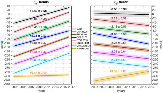
Figure 6.
Trends in χ1 and χ2 components of GAO, GSMAM, GRACE + SLR, and HAM + SLAM together with their errors. The shades show the errors of trends determined. The values are given in mas/year.
The overall seasonal time series of HAM and GAO are shown in Figure 7. For χ1 seasonal oscillations, GSMAM has quite smaller amplitudes than GAO and HAM + SLAM. In the case of χ2, amplitude differences between all GSMAM and GAO are even more visible. Interestingly, the χ2 HAM + SLAM series from the numerical models has almost the same magnitude as GAO.
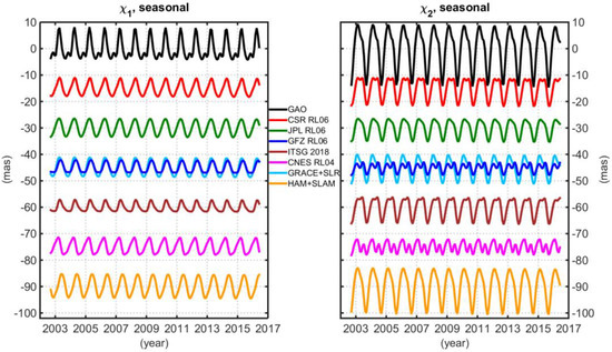
Figure 7.
Seasonal changes (sum of annual, semi-annual, and ter-annual oscillations, after removing linear trends) in χ1 and χ2 components of GAO, GSMAM, GRACE + SLR, and HAM + SLAM.
A common way to analyze seasonal oscillations is to present their phasor diagrams showing amplitudes and phases of prograde and retrograde terms of annual, semi-annual, and ter-annual oscillations related to reference epoch (in our study the reference epoch is January 2004). These phasor diagrams for annual and semi-annual variations are shown in Figure 8 and Figure 9, respectively, while the values of amplitudes and phases of seasonal (annual, semi-annual and ter-annual) oscillations and their errors are given in Table A2, Table A3 and Table A4 (Appendix A). In general, the length of each vector represents the magnitude of amplitude, while the vector direction shows a phase. The greater a difference between two vector directions, the more the time series are shifted relative to each other. The phase shift between two time series can affect the size of the correlation. The congruous length of two vectors indicates that these two time series are characterized by consistent magnitude of amplitudes.
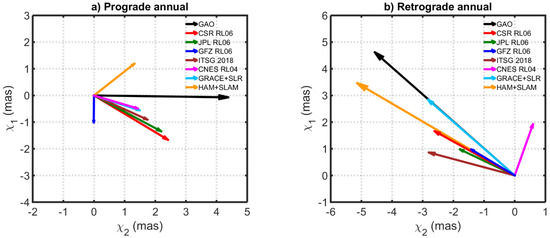
Figure 8.
Phasor diagrams of prograde and retrograde annual variation in χ1 + iχ2 for GAO, GSMAM, GRACE + SLR, and HAM + SLAM. Phase φ of the oscillation is defined by the annual term as sin(2π(t − t0) + φ), where t0 is the reference epoch (1 January 2004).
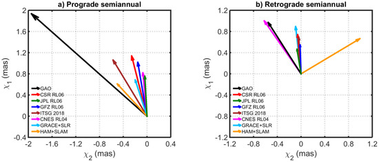
Figure 9.
Phasor diagrams of prograde and retrograde semi-annual variation in χ1 + iχ2 for GAO, GSMAM, GRACE + SLR, and HAM + SLAM. Phase φ of the oscillation is defined by the semi-annual term as sin(4π(t − t0) + φ), where t0 is the reference epoch (1 January 2004).
Naturally the annual oscillations (Figure 8) are stronger than semi-annual ones (Figure 9). The amplitude differences between GSMAM and GAO series shown in Figure 7 are reflected in inconsistencies in prograde and retrograde amplitudes (Figure 8 and Figure 9). Notably, HAM + SLAM and each GSMAM series underestimate annual and semi-annual amplitudes of GAO. For annual prograde term, the highest amplitude agreement with GAO is provided by GSMAM from CSR RL06 and JPL RL06, while for annual retrograde part the highest amplitude consistency with GAO is obtained for HAM + SLAM. Apart from GFZ RL06 in prograde and CNES RL04 in retrograde band, GSMAM annual phases are rather consistent with each other. Notably, GSMAM from CNES RL04 solution provides high amplitude and phase consistency in semi-annual retrograde part, but for semi-annual prograde term this agreement is one of the lowest. GSMAM from ITSG 2018 data reveals to provide the highest compatibility with GAO for semi-annual prograde part. For ter-annual oscillations, in general, the amplitude and phase values are highly questionable as in many cases the errors exceed the amplitude values (see Table A4 in Appendix A). Therefore, we do not consider ter-annual variations. The above findings highlight that it is difficult to conclude which GRACE solution provides the highest seasonal consistency with GAO as the results depend on what oscillations are considered (annual, semi-annual, or ter-annual; prograde or retrograde; amplitude or phase).
To analyze the agreement between non-seasonal GSMAM, GRACE + SLR, HAM + SLAM and GAO changes, we show time series of these oscillations (Figure 10), STD of the series, correlation coefficients and relative explained variance (Table 5). Figure 10 shows that there are some discrepancies between GSMAM from individual GRACE solutions, but the same amplitude peaks can be observed for all of them. Figure 10 also highlights a visible quasi-5-year oscillation in the χ2 component. Noticeably, the non-seasonal HAM + SLAM variations obtained from the geophysical models are rather smooth when compared to GRACE and GAO. However, the HAM + SLAM series represent the inter-annual variability in χ2 quite well. The values of STD given in Table 5 show that GSMAM series underestimate a variability of GAO in χ2, while STD of HAM + SLAM for this component is quite consistent with STD of GAO. The highest correlations with GAO for both χ1 and χ2 components are obtained for CNES RL04, but ITSG 2018 and CSR RL06 data also provide significant correlations which exceed 0.56 for χ1 and 0.64 for χ2. Accordingly, only these three solutions provide positive relative explained variances for both χ1 and χ2 and the best result is obtained for CNES RL04. Noticeably, the modelled HAM + SLAM series reveals sufficient correlation with GAO and high relative explained variance for χ2.
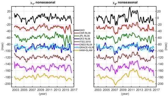
Figure 10.
Non-seasonal changes of χ1 and χ2 components of GAO, GSMAM, GRACE + SLR, and HAM + SLAM.
Table 5.
Standard deviation of non-seasonal GSMAM, GAO, GRACE + SLR, and HAM + SLAM time series, correlation coefficients with GAO, and percentage of variance in GAO explained by GSMAM, GRACE + SLR, and HAM + SLAM. The critical value of the correlation coefficient for 38 independent points and a confidence level of 0.95 is equal to 0.27. A standard error of a difference between two correlation coefficients for 38 independent points is equal to 0.24. The highest values of correlations and relative explained variances are italicized.
3.4. Analysis of GSMAM Series in Different Spectral Bands
We now extend our assessment to different spectral bands: (1) short-term changes with a period of 60–100 days, (2) a 100–450-day spectral band that includes periods of seasonal oscillations, and two longer-period spectral bands, namely (3) 450–1000 days, and (4) 1000–3000 days. This analysis aims to determine whether the level of agreement between GSMAM and GAO, between GRACE + SLAM and GAO or between HAM + SLAM and GAO depends on a specific spectral band in particular. The choice of spectral bands is determined by the length of available GRACE solutions, their monthly sampling, and the results of analysis of amplitude spectra of GAO, GSMAM and HAM + SLAM (Figure 3). These spectra show that, apart from strong seasonal oscillations, some longer-period variations occurs, namely with periods of around 450–1000 days and 1000–3000 days. Therefore, in the remainder of this paper, we consider these two spectral bands. Although we clearly indicated amplitude peaks for annual and semi-annual signals (see Figure 3), we decided to include them in one spectral band (100–450 days), since these changes were analyzed in detail already in Section 3.3. However, it should be noted that the 100–450-day range, apart from seasonal changes, also contains oscillations of both shorter and longer periods. Therefore, we cannot fully identify this spectral band with the seasonal changes analyzed in the previous chapter. To analyze short-term PM excitation, we introduce a spectral band of 60–100 days. It should be kept in mind that oscillations of higher frequencies cannot be considered due to monthly resolution of GRACE data. In this study, the oscillations in different spectral bands are calculated using a bandpass 4-pole Butterworth filter [63].
Figure 11a,b show long-term changes (with periods of 1000–3000 days) of GAO, GSMAM, GRACE + SLR and HAM + SLAM series, while the STD of time series, correlation coefficients with GAO and variance explained are presented in Table 6. Figure 11a shows that the χ1 series of HAM + SLAM is almost flat but the HAM + SLAM χ2 component shows the highest amplitude of all considered time series. Each GSMAM series underestimates STD of GAO for both χ1 and χ2 (Table 6). Nevertheless, there is good phase correspondence in χ2 between all considered data. For GAO, GSMAM and HAM + SLAM, we observe the same oscillation with the minimum amplitude peak at the end of 2007 and maximum amplitude peak at the beginning of 2011. Similar to non-seasonal variations (Figure 10), a visible quasi-5-year oscillation in the χ2 component is detected. In terms of correlation with GAO, the highest values for both χ1 and χ2 in the 1000–3000-day spectral band is obtained for ITSG 2018 and CSR RL06 data (Table 6). However, it should be noted that all GSMAM series perform very well in the case of χ2. As similar to the correlation results, the highest relative explained variances are observed for GSMAM from ITSG 2018 and CSR RL06 solutions (Table 6). Notably, the variance of the χ1 GAO component is explained by GRACE less accurately than χ2. However, all variances are positive for χ1 and only GFZ RL06 and CNES RL04 produce values that do not exceed 55%.
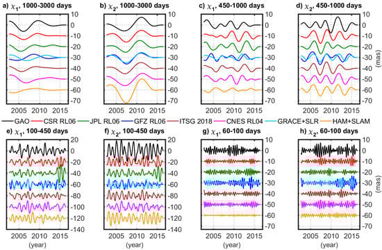
Figure 11.
Changes with the periods of 1000–4000 (a,b), 450–1000 (c,d), 100–450 (e,f), and 60–100 (g,h) days in χ1 and χ2 components of GAO, GSMAM, GRACE + SLR, and HAM + SLAM.
Table 6.
Standard deviation of GSMAM, GAO, GRACE + SLR, and HAM + SLAM time series, correlation coefficients with GAO, and percentage of variance in GAO explained by GSMAM, GRACE + SLR and HAM + SLAM. Oscillations with periods 1000–3000 days are considered. The critical value of the correlation coefficient for 9 independent points and a confidence level of 0.95 is equal to 0.58. The standard error of the difference between two correlation coefficients for the 9 independent points is equal to 0.58. The highest values of correlations and relative explained variances are italicized.
For the periods between 450 and 1000 days, we found that all series are rather consistent with each other in terms of amplitudes (apart from χ1 for HAM + SLAM), and the same amplitude peaks are visible for all of them (Figure 11c,d). Similar to the 1000–3000-day spectral band, χ1 of HAM + SLAM is distinguished by lower amplitudes than χ1 of GAO and GSMAM. Quasi-3-year changes in χ2 are visible in all series, which might be the result of groundwater variations. Compared to correlations with GAO and relative explained variances obtained for the 1000–3000-day spectral band, the values for 450–1000-day-changes are lower (Table 7). The best correlation and variance agreement with GAO is detected for GSMAM from CNES RL04 solution.
Table 7.
Standard deviation of GSMAM, GAO, GRACE + SLR, and HAM + SLAM time series, correlation coefficients with GAO, and percentage of variance in GAO explained by GSMAM, GRACE + SLR and HAM + SLAM. Oscillations with periods 450–1000 days are considered. The critical value of the correlation coefficient for 20 independent points and a confidence level of 0.95 is equal to 0.38. A standard error of a difference between two correlation coefficients for 20 independent points is equal to 0.34. The highest values of correlations and relative explained variances are italicized.
Figure 11e,f show GAO, GSMAM, GRACE + SLR and HAM + SLAM changes with periods between 100 and 450 days. Because these variations include, among others, also annual, semi-annual, and ter-annual oscillations, the series resemble sinusoids but with amplitudes of various sizes. Compared with longer oscillations, 100–450-day changes are noticeably stronger (note that the scale on the y axis is twice as large as that in Figure 11a–d). This is not surprising as seasonal oscillations have previously been shown to be the most powerful in hydrological PM excitation [15,28]. GSMAM and HAM + SLAM series reveal to underestimate the GAO variability since their STD values are lower than for the reference series, which is particularly evident in the case of χ2 (Table 8). The comparison of correlation coefficients with GAO and relative explained variances given in Table 8 shows that the highest agreement with GAO, for both χ1 and χ2 components, is observed for GSMAM from CSR RL06 solution, but satisfactory results are also noticeable for GSMAM from CNES RL04 and ITSG 2018. Notably, in χ2, HAM + SLAM series reveals to provide the highest consistency with GAO of all considered time series, with correlation of 0.76 and relative explained variance of 57%.
Table 8.
Standard deviation of GSMAM, GAO, GRACE + SLR, and HAM + SLAM time series, correlation coefficients with GAO, and percentage of variance in GAO explained by GSMAM, GRACE + SLR and HAM + SLAM. Oscillations with periods 100–450 days are considered. The critical value of the correlation coefficient for 59 independent points and a confidence level of 0.95 is equal to 0.22. A standard error of a difference between two correlation coefficients for 59 independent points is equal to 0.19. The highest values of correlations and relative explained variances are italicized.
Figure 11e,f show GAO, GSMAM, GRACE + SLR and HAM + SLAM changes with periods between 100 and 450 days. Because these variations include, among others, also annual, semi-annual, and ter-annual oscillations, the series resemble sinusoids but with amplitudes of various sizes. Compared with longer oscillations, 100–450-day changes are noticeably stronger (note that the scale on the y axis is twice as large as that in Figure 11a–d). This is not surprising as seasonal oscillations have previously been shown to be the most powerful in hydrological PM excitation [15,28]. GSMAM and HAM + SLAM series reveal to underestimate the GAO variability since their STD values are lower than for the reference series, which is particularly evident in the case of χ2 (Table 8). The comparison of correlation coefficients with GAO and relative explained variances given in Table 8 shows that the highest agreement with GAO, for both χ1 and χ2 components, is observed for GSMAM from CSR RL06 solution, but satisfactory results are also noticeable for GSMAM from CNES RL04 and ITSG 2018. Notably, in χ2, HAM + SLAM series reveals to provide the highest consistency with GAO of all considered time series, with correlation of 0.76 and relative explained variance of 57%.
The short-term GAO and GSMAM oscillations (with periods of 60–100 days) are shown in Figure 11g,h and the STD of the series, correlations with GAO, and relative explained variances are given in Table 9. The short-term variations reveal the smallest STD of all considered oscillations. Neither GSMAM nor HAM + SLAM series provide amplitudes and STD as high as for GAO. Notably, for GAO and GSMAM series there are some periods of stronger and some periods of weaker amplitudes, which is not observed for HAM + SLAM. The latter is characterized by the smallest amplitudes and STD among all the data considered. Taking into consideration correlation coefficients with GAO and relative explained variances (Table 9), we found that the best agreement with GAO for both χ1 and χ2 components is obtained when ITSG 2018, CNES RL04, or CSR RL06 are used. In general, it can be concluded that short-period oscillations can be described by GRACE with lower accuracy than other variations as correlation and relative explained variances are smaller than for longer-period changes. One of the reasons for the worse consistency between GAO and GSMAM in the short-term spectral band than in other considered bands, may be an aliasing of sub-daily signals in C04 EOP daily series.
Table 9.
Standard deviation of GSMAM, GAO, GRACE + SLR, and HAM + SLAM time series, correlation coefficients with GAO, and percentage of variance in GAO explained by GSMAM, GRACE + SLR and HAM + SLAM. Oscillations with periods 60–100 days are considered. The critical value of the correlation coefficient for 112 independent points and a confidence level of 0.95 is equal to 0.15. A standard error of a difference between two correlation coefficients for 112 independent points is equal to 0.14. The highest values of correlations and relative explained variances are italicized.
4. Discussion
The study reveals that, although the previous researches reported an improvement in consistency between particular GRACE solutions for RL06 compared to former RL05 release, and an increase of the agreement between GSMAM and GAO [37,57], the differences between particular GSMAM series are still remarkable. One of the sources of these discrepancies are different background models used to develop particular GRACE solutions. The biggest update in RL06 data concerns the change of mean pole model from cubic to linear in all solutions, which mostly affected GSMAM trends, but also might have a minor impact on long-term variability. In fact, the GSMAM trends from RL06 are more consistent with each other and with GAO trends than GSMAM trends from RL05 [15]. All the considered GRACE solutions use the same solid Earth tides model based on IERS Conventions (2010) [34] (see Table A1 in Appendix A). Each GRACE RL06 temporal model, except CNES RL04, introduced updated dealiasing product, namely AOD1B RL06 [35,36] instead of AOD1B RL05, which certainly benefited GSMAM in the short-term spectral band. However, while GSMAM from CSR RL06 and ITSG 2018 provide similar level of agreement with GAO for 60–100-day spectral band, GFZ RL06 and JPL RL06 reveal visibly lower correlations and relative explained variances for these oscillations. Moreover, CNES RL04 solution, which is not based on AOD1B RL06, provides results similar to those shown from CSR RL06 and ITSG 2018 data. The CNES RL04 dealiasing product uses the ERA-Interim (ECMWF Reanalysis from January 1989 onward) model for the atmospheric part, and the TUGO (Toulouse Unstructured Grid Ocean) barotropic model for the oceanic response to the ERA-interim pressure and wind forcing [51]. Nevertheless, the work of [37] showed that the update of dealiasing model in RL06 solutions played a minor role in GSMAM improving, while the change of mean pole model from cubic to linear had a great influence. Other background models, including mean gravity field models, ocean tides models or planetary ephemerides for perturbations induced by the large planets of the solar system, vary from one GRACE solution to another.
It should be kept in mind that apart from background models, GRACE solutions developed by various data centers differ from each other in terms of data processing algorithms and various parametrization schemes of accelerometers and K-band ranging, whose impact on PM excitation determination is hard to quantify. Moreover, not all details on the processing of GRACE observations have been made available to users by the data centers. Therefore, it is difficult to determine which processing algorithm or model used most contributed to the discrepancies between different GSMAM.
It is worth mentioning that, although the GRACE mission has come to an end, the leading GRACE data centers are still working on new RL07 solution that will cover the whole period of the mission duration. The data processing methods of new series will be consistent with those used to process observations of the successor of the GRACE mission, GRACE Follow-On, launched in May 2018. Therefore, future research on the topic and evaluation of new GRACE RL07 solutions should be conducted. Recently, in December 2019, the specialists from CNES/GRGS have developed their new release of GRACE solution, namely CNES/GRGS RL05, available at monthly and 10-day intervals. Moreover, there are other available types of GRACE data, such as terrestrial water storage (TWS) gridded data (GRACE Level-3 data) or local mass concentration (mascon) solutions [64] which are not considered here.
Moving back to the GRACE solutions provided by CNES/GRGS, it should be mentioned that, apart from the data from GRACE, they use also the data from SLR satellites, namely Starlette, Stella, Lageos, Lageos-2 and Ajisai [51]. These additional observations were exploited in order to improve the quality of the coefficients of very low degrees of the gravity field. This had an impact on improved agreement between GAO and GSMAM from CNES RL04. Indeed, compared to other GRACE solutions, CNES RL04 provides better results in non-seasonal and 450–1000-day spectral bands. However, GSMAM series from previous release of the solution, CNES RL03, was characterized by poor consistency with GAO [15].
The analyses of GSMAM trends presented in Section 3.2 and Section 3.3 reveal that, although the update of the mean pole model in GRACE RL06 data resulted in increased agreement between GSMAM and GAO trends, the full consistency is not achieved as GSMAM produced higher trends or both χ1 and χ2. Moreover, these characteristics depends on time period considered. Apart from the adopted mean pole model, applying the GIA model might also have an impact on the size of the trends in the PM excitation series obtained from GRACE. However, it should be kept in mind that the post-glacial rebound is not modelled in GRACE Level-2 data [31,33,65,66], with the exception of the CNES solutions for which GIA is taken into account by the a priori gravity field model [51,67]. The GIA model is included in GRACE Level-3 products (available via the GRACE Tellus website https://grace.jpl.nasa.gov/), which represent monthly mass changes given in grids. The former studies by our group [15] showed visible differences between trends of excitation series computed from GRACE Level-2 and Level-3 data. We found that the trends in the latter were noticeably smaller. However, in this paper we focus only on hydrological excitations computed directly from GRACE Level-2 GSM coefficients. As GIA is a long-term linear process, it does not influence the results for the period bands considered in this study.
During the analysis of non-seasonal time series conducted in the previous section, we detect a visible quasi-5-year oscillation in the χ2 (Figure 10) which is also noticeable in 1000–3000-day spectral band (Figure 11b). This oscillation might show the effects from groundwater change that was previously shown to affect mostly inter-annual PM excitation variability [68,69]. In fact, noticeable groundwater depletion is currently observed in many major aquifers [70]. As indicated in other research, the main driver of long-term and non-seasonal PM variation is also ice mass loss (e.g., 4). Since the beginning of the 21st century, ice mass loss has been observed in the Greenland and Antarctic ice sheets, mainly as a result of the warming climate [2,71]. However, the quasi-5-year oscillation is also noticeable for HAM + SLAM series, but LSDM, which is used to obtain HAM + SLAM series, includes only shallow groundwater layer and does not model the long-term ice mass changes in Greenland and Antarctica. Therefore, we expect that there are other drivers for this variation in PM excitation. The five-year change might be related to a change in continental water distribution due to different precipitation patterns. During 2007 and 2013 the trend in continental water distribution was different from the years before and after. It is not obvious, however, whether the variations in land water patterns relate to overall water mass (distribution between land and ocean) or a land-internal redistribution. Nevertheless, the signal is more pronounced in χ2 than in χ1, which more clearly indicates the direction of water exchange between land and ocean. Some authors suggested that electromagnetic core-mantle coupling also affects PM [72], but on decadal time scales, causing, for example, a Markowitz wobble with a period about 30 years [73].
It should be emphasized that for all considered oscillations, HAM + SLAM provides visibly higher consistency with GAO in χ2 than in χ1. While for χ1 HAM + SLAM reveals rather poor consistency with GAO compared to results from GRACE solutions, for χ2 this agreement is similar or even higher than for GSMAM. It should be kept in mind that χ2 might be more related to redistribution on the northern continents and between land and ocean, whereas χ1 could be more sensitive to ice or glacier mass changes. Therefore, it is unsurprising that a higher agreement between considered series is found in the case of χ2. We can therefore conclude that HAM + SLAM is able to model observed signals in PM at longer periods, which can provide an indication of liquid water and snow redistributions; however, it cannot model ice and glacier mass change. In fact, LSDM includes only the annual snow accumulation and melting on top of the glaciated regions.
5. Conclusions
In this paper, we evaluate GSMAM from the newest GRACE RL06 series of global gravity field models by comparing them with GAO derived from precise measurements of the pole coordinates. We also consider the combined GRACE + SLR solution as well as HAM + SLAM series computed from numerical models processed at GFZ. The trends, seasonal and non-seasonal changes, and oscillations in a number of different spectral bands are considered. GAO, GSMAM, GRACE + SLR and HAM + SLAM series are also analyzed at different time intervals, which are determined on the basis of different quality of GRACE data during these periods.
The study finds that the variability of both GAO and GSMAM as well as trends of the series are variable for different time intervals. Moreover, the consistency between GSMAM and GAO also varies between periods and is the highest in 2006–2014. GSMAM trends are consistent with each other but they overestimate the trends in GAO for both χ1 and χ2. The analyses show that for seasonal PM variations, it is difficult to identify the GRACE solutions that correspond best with GAO. For non-seasonal PM variations, the situation is clearer: the highest consistency with GAO are detected for the CNES RL04 solution.
We also identify the GRACE series that corresponds best with GAO in the chosen spectral bands and the results are as follows: (1) For 1000–3000-day oscillations, the highest correlation and variance agreement with GAO are observed for GSMAM from ITSG 2018 and CSR RL06 solutions. (2) For 450–1000-day changes, CNES RL04 is shown to provide the highest consistency between GSMAM and GAO. (3) In the 100–450-day spectral band, GSMAM computed from CSR RL06, ITSG 2018, and CNES RL04 solutions agree best with GAO. (4) For periods of of 60–100 days, the best correlation and variance agreement with GAO are observed for the ITSG 2018, CNES RL04, and CSR RL06 solutions. The level of agreement between GSMAM and GAO depend on the frequency band considered and is the highest for decadal changes with periods of 1000–3000 days and the lowest for short periods (60–100 days).
The results of this study demonstrate that there is no single solution that could give the highest consistency with GAO in all considered spectral bands. Nevertheless, the CSR RL06, ITSG 2018 and CNES RL04 appear to provide the best agreement with GAO for most of the oscillations investigated. However, it should be kept in mind that the latter use additional data from SLR satellites.
This study shows that the combination of GRACE and SLR, which is recommended during the use of C21, S21 coefficients from GFZ RL06 data, improves the consistency between GSMAM and GAO. The formal errors of GRACE + SLR solution are smaller than errors of any GSMAM series. The combined series are also less noisy than GFZ RL06, especially in the last period of GRACE satellites activity. However, despite the fact that GRACE + SLR provides clearly better consistency with GAO than GSMAM from GFZ RL06, it does not perform as well as CSR RL06. GRACE + SLR results represents rather the mean of results obtained from considered GRACE solutions.
We note that the HAM + SLAM series from the numerical models processed at GFZ is unable to provide such high correlations with GAO as the GSMAM data, especially in χ1. Similar findings have been shown in previous studies by our group, where different hydrological and climate models were compared with gravimetric measurements and geodetic excitations [14,15,17,30]. LSDM-based hydrological excitations are found to be affected by weaknesses especially in χ1 of 450–1000 and 60–100-day spectral bands. However, [15] showed that LSDM gives more satisfactory results than other hydrological and climate models. This study shows that the results obtained from HAM + SLAM are comparable with those provided by GRACE solutions at the 100–450-day and seasonal bands. Moreover, if only χ2 would be considered, it will be found that HAM + SLAM provides one of the best results for all oscillations and time intervals considered.
Finally, it should be emphasized that none of the considered data sets are free of errors. The GAO series, which is taken as our reference for the quality assessment of GRACE- and model-based PM excitations, is affected by uncertainties of atmospheric and ocean models, while GRACE data are influenced by the errors in background models. Another method to assess uncertainties in hydrological excitations from different GRACE solutions, might be the estimating the noise in the series, using the three-cornered hat method, for example [74,75]. However, this could provide only internal agreement between different GRACE series since no external data are used. Nevertheless, such an assessment would be free of errors in atmosphere and ocean models used for GAO computation. Hopefully, the successor of the GRACE mission, GRACE Follow-On with the innovative Laser Ranging Interferometer to be used for the satellite-to-satellite tracking, will provide determinations of temporal Earth’s gravity field changes with a higher quality than available so far, which also could improve the estimation of gravimetric excitation from satellite missions.
Author Contributions
Conceptualization, J.Ś.; data curation, J.Ś., H.D. and R.D.; formal analysis, J.Ś.; funding acquisition, J.Ś. and J.N.; investigation, J.Ś.; methodology, J.Ś. and J.N.; project administration, J.Ś. and J.N.; resources, J.Ś., H.D. and R.D.; software, J.Ś.; supervision, J.Ś. and J.N.; validation, H.D. and R.D.; visualization, J.Ś.; writing—original draft, J.Ś.; writing—review and editing, J.Ś., J.N., H.D. and R.D. All authors have read and agreed to the published version of the manuscript.
Funding
This research was funded by National Science Center, Poland (NCN), grant number 2018/31/N/ST10/00209, and by the Polish National Agency for Academic Exchange (NAWA) grant number PPI/APM/2018/1/00032/U/001.
Acknowledgments
We would like to thank three anonymous Reviewers for their valuable comments that contributed to the improvement of the article.
Conflicts of Interest
The authors declare no conflict of interest.
Appendix A
Table A1.
Background models, data sources, and references for temporal GRACE gravity field models.
Table A1.
Background models, data sources, and references for temporal GRACE gravity field models.
| Temporal Gravity Field Model | Mean Gravity Field Model | N body Perturbations | Pole Tides | Ocean Tides | Atmospheric and Oceanic Non-Tidal Mass Variations | Data Source | Reference |
|---|---|---|---|---|---|---|---|
| CSR RL05 | GIF48 | DE 405 | IERS 2010 (cubic) | GOT4.8 | AOD1B RL05 | https://podaac-tools.jpl.nasa.gov/drive/files/GeodeticsGravity/grace/L2 | [64] |
| CSR RL06 | GGM05C | DE 430 | IERS 2010 (linear) | GOT4.8 | AOD1B RL06 | https://podaac-tools.jpl.nasa.gov/drive/files/GeodeticsGravity/grace/L2 | [31] |
| JPL RL05 | GIF48 | DE 421 | IERS 2010 (cubic) | GOT4.7 | AOD1B RL05 | https://podaac-tools.jpl.nasa.gov/drive/files/GeodeticsGravity/grace/L2 | [65] |
| JPL RL06 | GGM05C | DE 430 | IERS 2010 (linear) | FES2014b | AOD1B RL06 | https://podaac-tools.jpl.nasa.gov/drive/files/GeodeticsGravity/grace/L2 | [33] |
| GFZ RL05 | EIGEN-6C | DE 421 | Constant mean pole | EOT11a | AOD1B RL05 | https://podaac-tools.jpl.nasa.gov/drive/files/GeodeticsGravity/grace/L2 | [76] |
| GFZ RL06 | EIGEN-6C4 | DE 430 | IERS 2010 (linear) | FES2014 | AOD1B RL06 | https://podaac-tools.jpl.nasa.gov/drive/files/GeodeticsGravity/grace/L2 | [32,49] |
| ITSG 2016 | GOCO04s | DE 421 | IERS 2010 (cubic) | EOT11a | AOD1B RL05 | http://icgem.gfz-potsdam.de/home | [77] |
| ITSG 2018 | ITSG-GraceGoce2017 | DE 421 | IERS 2010 (linear) | FES2014b + GRACE | AOD1B RL06 + LSDM | http://icgem.gfz-potsdam.de/home | [50] |
| CNES RL03 | EIGEN-GRGS.RL03-v2.MEAN-FIELD | DE 405 | IERS 2010 (cubic) | FES2012 | ECMWF ERA-Interim (atmosphere) + TUGO (ocean) | http://grgs.obs-mip.fr/grace | [66] |
| CNES RL04 | EIGEN-GRGS.RL03-v2.MEAN-FIELD | DE 405 | IERS 2010 (linear) | FES2014 | ECMWF ERA-Interim (atmosphere) + TUGO (ocean) | http://grgs.obs-mip.fr/grace | [51] |
Solid Earth Tides for all solutions were based on the IERS Conventions (2010) [34].
Table A2.
Amplitudes and phases of prograde and retrograde annual oscillations of GAO, GSM, and HAM + SLAM together with their errors. The phases refer to the reference epoch starting on 1 January 2004.
Table A2.
Amplitudes and phases of prograde and retrograde annual oscillations of GAO, GSM, and HAM + SLAM together with their errors. The phases refer to the reference epoch starting on 1 January 2004.
| Series | Annual Amplitudes | Annual Phases | ||
|---|---|---|---|---|
| Prograde Amplitude (mas) | Retrograde Amplitude (mas) | Prograde Phase (°) | Retrograde Phase (°) | |
| GAO | 4.38 ± 0.80 | 6.49 ± 1.01 | −1 ± 4 | +135 ± 3 |
| CSR RL06 | 2.93 ± 0.89 | 3.10 ± 0.90 | −35 ± 5 | +148 ± 6 |
| JPL RL06 | 2.57 ± 0.78 | 2.76 ± 0.83 | −32 ± 3 | +130 ± 6 |
| GFZ RL06 | 1.01 ± 0.84 | 1.72 ± 0.92 | −90 ± 5 | +145 ± 6 |
| ITSG 2018 | 1.97 ± 1.02 | 2.93 ± 1.22 | −27 ± 3 | +163 ± 2 |
| CNES RL04 | 1.51 ± 0.83 | 2.01 ± 0.89 | −19 ± 5 | +73 ± 5 |
| GRACE + SLR | 1.59 ± 0.60 | 4.01 ± 0.61 | −21 ± 3 | +134 ± 2 |
| HAM + SLAM | 1.78 ± 1.00 | 6.19 ± 1.11 | +42 ± 4 | +146 ± 3 |
Table A3.
Amplitudes and phases of prograde and retrograde semi-annual oscillations of GAO, GSM, and HAM + SLAM together with their errors. The phases refer to the reference epoch starting on 1 January 2004.
Table A3.
Amplitudes and phases of prograde and retrograde semi-annual oscillations of GAO, GSM, and HAM + SLAM together with their errors. The phases refer to the reference epoch starting on 1 January 2004.
| Series | Semi-Annual Amplitudes | Semi-Annual Phases | ||
|---|---|---|---|---|
| Prograde Amplitude (mas) | Retrograde Amplitude (mas) | Prograde Phase (°) | Retrograde Phase (°) | |
| GAO | 2.74 ± 0.81 | 1.12 ± 0.91 | +135 ± 8 | +120 ± 9 |
| CSR RL06 | 1.17 ± 0.78 | 0.74 ± 0.49 | +103 ± 7 | +94 ± 6 |
| JPL RL06 | 0.76 ± 0.72 | 0.47 ± 0.32 | +93 ± 5 | +98 ± 4 |
| GFZ RL06 | 1.03 ± 0.88 | 0.55 ± 0.32 | +99 ± 6 | +92 ± 6 |
| ITSG 2018 | 1.20 ± 0.80 | 0.69 ± 0.69 | +118 ± 10 | +93 ± 11 |
| CNES RL04 | 0.82 ± 0.70 | 1.18 ± 0.69 | +95 ± 6 | +122 ± 5 |
| GRACE + SLR | 0.71 ± 0.69 | 0.90 ± 0.65 | +106 ± 5 | +96 ± 4 |
| HAM + SLAM | 0.79 ± 0.52 | 1.19 ± 0.69 | +129 ± 12 | +34 ± 9 |
Table A4.
Amplitudes and phases of prograde and retrograde ter-annual oscillations of GAO, GSM, and HAM + SLAM together with their errors. The phases refer to the reference epoch starting on 1 January 2004.
Table A4.
Amplitudes and phases of prograde and retrograde ter-annual oscillations of GAO, GSM, and HAM + SLAM together with their errors. The phases refer to the reference epoch starting on 1 January 2004.
| Series | Ter-Annual Amplitudes | Ter-Annual Phases | ||
|---|---|---|---|---|
| Prograde Amplitude (mas) | Retrograde Amplitude (mas) | Prograde Phase (°) | Retrograde Phase (°) | |
| GAO | 0.36 ± 0.71 | 1.12 ± 0.78 | −142 ± 15 | −102 ± 11 |
| CSR RL05 | 0.29 ± 0.57 | 0.31 ± 0.48 | −34 ± 15 | −89 ± 18 |
| JPL RL06 | 0.09 ± 0.50 | 0.06 ± 0.39 | −131 ± 19 | −36 ± 22 |
| GFZ RL06 | 0.15 ± 0.40 | 0.23 ± 0.39 | −88 ± 8 | −128 ± 11 |
| ITSG 2018 | 0.14 ± 0.61 | 0.33 ± 0.40 | −45 ± 19 | −93 ± 27 |
| CNES RL04 | 0.27 ± 0.59 | 0.62 ± 0.42 | −78 ± 12 | −82 ± 15 |
| GRACE + SLR | 0.01 ± 0.49 | 0.15 ± 0.50 | +18 ± 18 | −155 ± 30 |
| HAM + SLAM | 0.40 ± 0.50 | 0.34 ± 0.46 | −57 ± 15 | −90 ± 18 |
References
- Lambeck, K. The Earth’s Variable Rotation: Geophysical Causes and Consequences; Cambridge University Press: Cambridge, UK, 1980. [Google Scholar]
- Adhikari, S.; Ivins, E.R. Climate–driven polar motion: 2003–2015. Sci. Adv. 2016, 2, e1501693. [Google Scholar] [CrossRef] [PubMed]
- Adhikari, S.; Caron, L.; Steinberger, B.; Reager, J.T.; Kjeldsen, K.K.; Marzeion, B.; Larour, E.; Ivins, E.R. What drives 20th century polar motion? Earth Planet. Sci. Lett. 2018, 502, 126–132. [Google Scholar] [CrossRef]
- Youm, K.; Seo, K.W.; Jeon, T.; Na, S.H.; Chen, J.; Wilson, C.R. Ice and groundwater effects on long term polar motion (1979–2010). J. Geodyn. 2017, 106, 66–73. [Google Scholar] [CrossRef]
- Tapley, B.; Watkins, M.M.; Flechtner, F.; Reigber, C.; Bettadpur, S.; Rodell, M.; Famiglietti, J.; Landerer, F.; Chambers, D.; Reager, J.; et al. Contributions of GRACE to understanding climate change. Nat. Clim. Chang. 2019, 9, 358–369. [Google Scholar] [CrossRef]
- Gross, R. Theory of earth rotation variations. In VIII Hotine-Marussi Symposium on Mathematical Geodesy; Sneeuw, N., Novák, P., Crespi, M., Sansò, F., Eds.; Springer: Cham, Switzerland, 2015; Volume 142. [Google Scholar]
- Brzeziński, A.; Nastula, J.; Kołaczek, B.; Ponte, R.M. Oceanic excitation of polar motion from interannual to decadal periods. In Proceedings of the International Association of Geodesy, IAG General Assembly, Sapporo, Japan, 30 June–11 July 2003. [Google Scholar]
- Brzeziński, A.; Nastula, J.; Kołaczek, B. Seasonal excitation of polar motion estimated from recent geophysical models and observations. J. Geodyn. 2009, 48, 235–240. [Google Scholar] [CrossRef]
- Gross, R.S.; Fukumori, I.; Menemenlis, D. Atmospheric and oceanic excitation of the Earth’s wobbles during 1980–2000. J. Geophys. Res. Solid Earth 2003, 108, 2370. [Google Scholar] [CrossRef]
- Nastula, J.; Ponte, R.M. Further evidence for oceanic excitation of polar motion. Geophys. J. Int. 1999, 139, 123–130. [Google Scholar] [CrossRef]
- Nastula, J.; Ponte, R.M.; Salstein, D.A. Regional signals in atmospheric and oceanic excitation of polar motion. In Polar Motion: Historical and Scientific Problems; Dick, S., McCarthy, D., Luzum, B., Eds.; Astronomical Society of the Pacific: San Francisco, CA, USA, 2000; pp. 463–472. [Google Scholar]
- Nastula, J.; Ponte, R.M.; Salstein, D.A. Comp on excitation series derived from GRACE and from analyses of geophysical fluids. Geophys. Res. Lett. 2007, 34, 2–7. [Google Scholar] [CrossRef]
- Nastula, J.; Salstein, D.A.; Kołaczek, B. Patterns of atmospheric excitation functions of polar motion from high–resolution regional sectors. J. Geophys. Res. 2009, 114, B04407. [Google Scholar] [CrossRef]
- Nastula, J.; Pasnicka, M.; Kolaczek, B. Comparison of the geophysical excitations of polar motion from the period 1980.0–2007.0. Acta Geophys. 2011, 59, 561–577. [Google Scholar] [CrossRef]
- Nastula, J.; Wińska, M.; Śliwińska, J.; Salstein, D. Hydrological signals in polar motion excitation—Evidence after fifteen years of the GRACE mission. J. Geodyn. 2019, 124, 119–132. [Google Scholar] [CrossRef]
- Seoane, L.; Nastula, J.; Bizouard, C.; Gambis, D. Hydrological excitation of polar motion derived from GRACE gravity field solutions. Int. J. Geophys. 2011. [Google Scholar] [CrossRef]
- Śliwińska, J.; Wińska, M.; Nastula, J. Terrestrial water storage variations and their effect on polar motion. Acta Geophys. 2019, 67, 17–39. [Google Scholar] [CrossRef]
- Wińska, M.; Nastula, J.; Salstein, D.A. Hydrological excitation of polar motion by different variables from the GLDAS model. J. Geod. 2017, 17, 7110. [Google Scholar] [CrossRef]
- Gross, R.S.; Chao, B.F. The rotational and gravitational signature of the December 26, 2004 Sumatran earthquake. Surv. Geophs. 2006, 27, 615–632. [Google Scholar] [CrossRef]
- Greiner-Mai, H. Decade Variations of the Earth’s Rotation and Geomagnetic Core-Mantle Coupling. J. Geomagn. Geoelectr. 1993, 45, 1333–1345. [Google Scholar] [CrossRef]
- Greiner-Mai, H.; Jochmann, H.; Barthelmes, F. Influence of possible inner–core motions on the polar motion and the gravity field. Phys. Earth Planet. Inter. 2000, 117, 81–93. [Google Scholar] [CrossRef]
- Tapley, B.D.; Bettadpur, S.; Watkins, M.; Reigber, C. The gravity recovery and climate experiment: Mission overview and early results. Geophys. Res. Lett. 2004, 31, 1–4. [Google Scholar] [CrossRef]
- Mitrovica, J.X.; Milne, G.A.; Davis, J.L. Glacial isostatic adjustment on a rotating earth. Geophys. J. Int. 2001, 147, 562–578. [Google Scholar] [CrossRef]
- Chambers, D.P.; Wahr, J.; Nerem, R.S. Preliminary observations of global ocean mass variations with GRACE. Geophys. Res. Lett. 2004, 31, 1–4. [Google Scholar] [CrossRef]
- Han, S.C.; Shum, C.K.; Bevis, M.; Ji, C.; Kuo, C.Y. Crustal dilatation observed by GRACE after the 2004 Sumatra–Andaman earthquake. Science 2006, 313, 658–662. [Google Scholar] [CrossRef] [PubMed]
- Jin, S.; Chambers, D.P.; Tapley, B.D. Hydrological and oceanic effects on polar motion from GRACE and models. J. Geophys. Res. 2010, 115, B02403. [Google Scholar] [CrossRef]
- Jin, S.; Hassan, A.A.; Feng, G.P. Assessment of terrestrial water contributions to polar motion from GRACE and hydrological models. J. Geodyn. 2012, 62, 40–48. [Google Scholar] [CrossRef]
- Chen, J.L.; Wilson, C.R.; Zhou, Y.H. Seasonal excitation of polar motion. J. Geodyn. 2012, 62, 8–15. [Google Scholar] [CrossRef]
- Nastula, J.; Salstein, D.A.; Popiński, W. Hydrological excitations of polar motion from GRACE gravity field solutions. Int. Assoc. Geod. Symp. 2016, 513–519. [Google Scholar] [CrossRef]
- Wińska, M.; Nastula, J.; Kołaczek, B. Assessment of the global and regional land hydrosphere and its impact on the balance of the geophysical excitation function of polar motion. Acta Geophys. 2016, 64, 1–23. [Google Scholar] [CrossRef]
- Bettadpur, S. UTCSR Level–2 Processing Standards Document for Level–2 Product Release 0006. Technical Report GRACE 2018. Available online: http://icgem.gfz-potsdam.de/GRACE_CSR_L2_Processing_Standards_Document_for_RL06.pdf (accessed on 24 December 2019).
- Dahle, C.; Flechtner, F.; Murböck, M.; Michalak, G.; Neumayer, H.; Abrykosov, O.; Reinhold, A.; König, R. GFZ Level-2 Processing Standards Document for Level-2 Product Release 06. Scientific Technical Report STR-Data. 2019. Available online: http://icgem.gfz-potsdam.de/GRACE_GFZ_L2_Processing_Standards_Document_for_RL06.pdf (accessed on 24 December 2019).
- Yuan, D. JPL level–2 Processing Standards Document for Level–2 Product Release 06. Technical Report GRACE, 327–744. Available online: http://icgem.gfz-potsdam.de/GRACE_JPL_L2_Processing_Standards_Document_for_RL06.pdf (accessed on 24 December 2019).
- Petit, G.; Luzum, B. IERS Conventions; Bureau International Des Poids et Mesures Sevres: Frankfurt am Main, Germany, 2010. [Google Scholar]
- Dobslaw, H.; Wolf, I.; Dill, R.; Poropat, L.; Thomas, M.; Dahle, C.; Esselborn, S.; König, R.; Flechtner, F. A new high–resolution model of non–tidal atmosphere and ocean mass variability for de–aliasing of satellite gravity observations: AOD1B RL06. Geophys. J. Int. 2017, 211, 263–269. [Google Scholar] [CrossRef]
- Dobslaw, H.; Bergmann-Wolf, I.; Dill, R.; Poropat, L.; Flechtner, F. Product Description Document for AOD1B Release 06. Technical Report GRACE, 327–750. Available online: Ftp://isdcftp.gfz-potsdam.de/grace/DOCUMENTS/Level-1/ (accessed on 24 December 2019).
- Göttl, F.; Schmidt, M.; Seitz, F. Mass–related excitation of polar motion: An assessment of the new RL06 GRACE gravity field models. Earth Planets Space 2018, 70. [Google Scholar] [CrossRef]
- Brzezinski, A. Polar motion excitation by variations of the effective angular momentum function: Considerations concerning deconvolution problem. Manuscr. Geod. 1992, 17, 3–20. [Google Scholar]
- Eubanks, T.M. Variations in the orientation of the Earth. In Contributions of Space Geodesy to Geodynamics: Earth Dynamics: Geodynamic Series; Smith, D.E., Turcotte, D.L., Eds.; American Geophysical Union: Washington, DC, USA, 1993; Volume 24, pp. 1–54. [Google Scholar]
- Bizouard, C.; Lambert, S.; Becker, O.; Richard, J.Y. Combined solution C04 for Earth Rotation Parameters consistent with International Terrestrial Reference Frame 2014. IERS Notice. Available online: http://hpiers.obspm.fr/eoppc/eop/eopc04/C04.guide.pdf (accessed on 24 December 2019).
- Bizouard, C.; Lambert, S.; Gattano, C.; Becker, O.; Richard, J.Y. The IERS EOP 14C04 solution for Earth orientation parameters consistent with ITRF 2014. J. Geod. 2018, 93, 621. [Google Scholar] [CrossRef]
- Naito, I.; Zhou, Y.-H.; Sugi, M.; Kawamura, R.; Sato, N. Three–dimensional Atmospheric Angular Momentum Simulated by the Japan Meteorological Agency model for the period of 1955–1994. J. Meteorol. Soc. Jpn. 2000, 78, 111–122. [Google Scholar] [CrossRef][Green Version]
- Zhou, Y.H.; Chen, J.L.; Liao, X.H.; Wilson, C.R. Oceanic excitations on polar motion: A cross comparison among models. Geophys. J. Int. 2005, 162, 390–398. [Google Scholar] [CrossRef]
- Vondrak, J.; Ron, C. Geophysical fluids, geomagnetic jerks, and their impact on Earth orientation. Publ. Astron. Obs. Belgrade 2017, 96, 51–60. [Google Scholar]
- Dobslaw, H.; Dill, R.; Grötzsch, A.; Brzeziński, A.; Thomas, M. Seasonal polar motion excitation from numerical models of atmosphere, ocean, and continental hydrosphere. J. Geophys. Res. 2010, 115, B10406. [Google Scholar] [CrossRef]
- Jungclaus, J.H.; Fischer, N.; Haak, H.; Lohmann, K.; Marotzke, J.; Matei, D.; Mikolajewicz, U.; Notz, D.; vonStorch, J.S. Characteristics of the ocean simulations in MPIOM, the ocean component of the MPI-Earth system model. J. Adv. Model. Earth Syst. 2013, 5, 422–446. [Google Scholar] [CrossRef]
- Altamimi, Z.; Rebischung, P.; Métivier, L.; Collilieux, X. ITRF2014: A new release of the International Terrestrial Reference Frame modeling nonlinear station motions. J. Geophys. Res. Solid Earth 2016, 121, 6109–6131. [Google Scholar] [CrossRef]
- Fey, A.L.; Gordon, D.; Jacobs, C.S.; Ma, C.; Gaume, R.A.; Arias, E.F.; Bianco, G.; Boboltz, D.A.; Böckmann, S.; Bolotin, S. The second realization of the international celestial reference frame by very long baseline interferometry. Astron. J. 2015, 2, 58. [Google Scholar] [CrossRef]
- Dahle, C.; Murböck, M.; Flechtner, F.; Dobslaw, H.; Michalak, G.; Neumayer, K.H.; Abrykosov, O.; Reinhold, A.; König, R.; Sulzbach, R.; et al. The GFZ GRACE RL06 monthly gravity field time series: Processing details and quality assessment. Remote Sens. 2019, 11, 2116. [Google Scholar] [CrossRef]
- Mayer-Gürr, T.; Behzadpour, S.; Ellmer, M.; Kvas, A.; Klinger, B.; Strasser, S.; Zehentner, N. ITSG-Grace2018-Monthly, Daily and Static Gravity Field Solutions from GRACE. GFZ Data Services. Available online: http://dataservices.gfz-potsdam.de/icgem/showshort.php?id=escidoc:3600910 (accessed on 24 December 2019).
- Lemoine, J.-M.; Bourgogne, S.; Biancale, R.; Gégout, P. The new GRGS–RL04 series of mass variations modelled with GRACE data. In Proceedings of the 20th EGU General Assembly, Vienna, Austria, 4–13 April 2018. [Google Scholar]
- Dill, R. Hydrological Model LSDM for Operational Earth Rotation and Gravity Field Variations. GFZ Scientific Technical Report STR; 08/09. Available online: http://gfzpublic.gfz-potsdam.de/pubman/item/escidoc:8770 (accessed on 24 December 2019).
- Dill, R. Hydrological induced Earth rotation variations from standalone and dynamically coupled simulations. In Proceedings of the Journées 2008 Systèmes de Référence Spatio-Temporels, Dresden, Germany, 22–24 September 2008. [Google Scholar]
- Dobslaw, H.; Dill, R. Effective Angular Momentum Functions from Earth System Modelling at GeoForschungsZentrum in Potsdam. Technical Report, Revision 1.1 (March 18, 2019), GFZ Potsdam, Germany. Available online: http://rz-vm115.gfz-potsdam.de:8080/repository (accessed on 24 December 2019).
- Meyrath, T.; van Dam, T. A comparison of interannual hydrological polar motion excitation from GRACE and geodetic observations. J. Geodyn. 2016, 99, 1–9. [Google Scholar] [CrossRef]
- Bizouard, C. Elliptic polarisation of the polar motion excitation. J. Geod. 2016, 90, 179–188. [Google Scholar] [CrossRef]
- Nastula, J.; Śliwińska, J. Prograde and Retrograde Terms of Gravimetric Polar Motion Excitation Estimates from the GRACE Monthly Gravity Field Models. Remote Sens. 2020, 12, 138. [Google Scholar] [CrossRef]
- Kosek, W. Time Variable Band Pass Filter Spectra of Real and Complex-Valued Polar Motion Series. Artif. Satell. 1995, 30, 27–43. [Google Scholar]
- Śliwińska, J.; Nastula, J. Determining and Evaluating the Hydrological Signal in Polar Motion Excitation from Gravity Field Models Obtained from Kinematic Orbits of LEO Satellites. Remote Sens. 2019, 11, 1784. [Google Scholar] [CrossRef]
- Chen, W.; Li, J.; Ray, J.; Cheng, M. Improved geophysical excitations constrained by polar motion observations and GRACE/SLR time-dependent gravity. Geod. Geodyn. 2017, 8, 377–388. [Google Scholar] [CrossRef]
- Seoane, L.; Biancale, R.; Gambis, D. Agreement between Earth’s rotation and mass displacement as detected by GRACE. J. Geodyn. 2012, 62, 49–55. [Google Scholar] [CrossRef]
- Wińska, M.; Śliwińska, J. Assessing hydrological signal in polar motion from observations and geophysical models. Stud. Geophys. Geod. 2019, 63, 95–117. [Google Scholar] [CrossRef]
- Bianchi, G.; Sorrentino, R. Electronic Filter Simulation & Design; McGraw-Hill Professional: New York, NY, USA, 2007; pp. 17–20. [Google Scholar]
- Watkins, M.M.; Wiese, D.N.; Yuan, D.-N.; Boening, C.; Landerer, F.W. Improved methods for observing Earth’s time variable mass distribution with GRACE using spherical cap mascons. J. Geophys. Res. Solid Earth 2015, 120, 2648–2671. [Google Scholar] [CrossRef]
- Bettadpur, S. UTCSR Level-2 Processing Standards Document for Level-2 Product Release 0005. Technical Report GRACE 2012. Available online: http://icgem.gfz-potsdam.de/L2-CSR0005_ProcStd_v4.0.pdf (accessed on 24 December 2019).
- Watkins, M.M.; Yuan, D. JPL Level-2 Processing Standards Document for Level-2 Product Release 05.1. Technical Report GRACE. Available online: http://icgem.gfz-potsdam.de/L2-JPL_ProcStds_v5.1.pdf (accessed on 24 December 2019).
- Lemoine, J.-M.; Bourgogne, S.; Bruinsma, S.; Gégout, P.; Reinquin, F.; Biancale, R. GRACE RL03–v2 monthly time series of solutions from CNES/GRGS. In Proceedings of the 17th EGU General Assembly, Vienna, Austria, 12–17 April 2018. [Google Scholar]
- Güntner, A. Improvement of global hydrological models using GRACE data. Surv. Geophys. 2008, 29, 375–397. [Google Scholar] [CrossRef]
- Güntner, A.; Stuck, J.; Werth, S.; Döll, P.; Verzano, K.; Merz, B. A global analysis of temporal and spatial variations in continental water storage. Water Resour. Res. 2007, 43, 1–19. [Google Scholar] [CrossRef]
- Wada, Y.; Van Beek, L.P.H.; Van Kempen, C.M.; Reckman, J.W.T.M.; Vasak, S.; Bierkens, M.F.P. Global depletion of groundwater resources. Geophys. Res. Lett. 2010, 37, 1–5. [Google Scholar] [CrossRef]
- Velicogna, I.; Sutterley, T.C.; Van Den Broeke, M.R. Regional acceleration in ice mass loss from Greenland and Antarctica using GRACE time-variable gravity data. Geophys. Res. Lett. 2014, 41, 8130–8137. [Google Scholar] [CrossRef]
- Kuang, W.; Chao, B.F.; Chen, J. Decadal polar motion of the Earth excited by the convective outer core from geodynamo simulations. J. Geophys. Res. Solid Earth 2017, 122, 8459–8473. [Google Scholar] [CrossRef]
- Poma, A. The Markowitz Wobble. In Polar Motion: Historical and Scientific Problems; Dick, S., McCarthy, D., Luzum, B., Eds.; Astronomical Society of the Pacific: San Francisco, CA, USA, 2000; pp. 351–354. [Google Scholar]
- Premoli, A.; Tavella, P. A revisited three-cornered hat method for estimating frequency standard instability. IEEE Trans. Meas. 1993, 42, 7–13. [Google Scholar] [CrossRef]
- Koot, L.; Viron, O.; Dehant, V. Atmospheric Angular Momentum Time-Series: Characterization of their Internal Noise and Creation of a Combined Series. J. Geod. 2006, 79, 663. [Google Scholar] [CrossRef]
- Dahle, C.; Flechtner, F.; Gruber, C.; König, D.; König, R.; Michalak, G.; Neumayer, K.H. GFZ GRACE Level–2 Processing Standards Document for Level–2 Product Release 0005. Scientific Technical Report STR12/02–data, Revised Edition. Available online: http://icgem.gfz-potsdam.de/L2-GFZ_ProcStds_0005_v1.1-1.pdf (accessed on 24 December 2019).
- Mayer-Gürr, T.; Behzadpour, S.; Ellmer, M.; Kvas, A.; Klinger, B.; Zehentner, N. ITSG-Grace2016-Monthly and Daily Gravity Field Solutions from GRACE. GFZ Data Services. Available online: http://dataservices.gfz-potsdam.de/icgem/showshort.php?id=escidoc:1697893 (accessed on 24 December 2019).
© 2020 by the authors. Licensee MDPI, Basel, Switzerland. This article is an open access article distributed under the terms and conditions of the Creative Commons Attribution (CC BY) license (http://creativecommons.org/licenses/by/4.0/).