1. Introduction
Strong El Nino Southern Oscillation (ENSO) events are closely related to the interannual variability of tropical oceans. The interannual variability of the atmosphere and oceans may result from the self-sustained oscillation of the atmosphere–ocean coupling within a period of 3–5 years, as based on numerical simulations of tropical regions [
1,
2,
3,
4,
5,
6,
7,
8,
9,
10]. This coupling system may be better explained as a delayed action oscillator (DAO) that combines positive and delayed negative feedback of the sea surface temperature (SST) in the tropical Pacific [
6]. In this coupling process, a positive sea surface temperature anomaly in the equatorial eastern Pacific causes westerly wind anomalies that produce a downwelling Kelvin wave in the equatorial central Pacific. The downwelling Kelvin wave propagates eastward, and then reflected by the eastern boundary of the equatorial Pacific, it becomes an upwelling Rossby wave which travels westward. The downwelling Kelvin wave deepens the thermocline in the eastern Pacific and increases the surface temperature, which in turn weakens the Walker circulation and reinforces westerly wind anomalies, thus inducing a positive feedback. When the Rossby wave reaches the western boundary of the equatorial Pacific, it is reflected and becomes an upwelling Kelvin wave propagating westward. The upwelling Kelvin wave then imposes a negative feedback on positive sea surface temperature anomalies via shallowing of the deepened thermocline caused by the downwelling Kelvin wave. This delayed action of the upwelling Kelvin wave brings the warm event back to equilibrium and sometimes induces a cooling event (i.e., La Nina). ENSO-like inter-decadal variability has been found in long-term simulations of the atmosphere–ocean coupling [
8,
11] and has also been observed in sea surface temperature data [
12].
It is believed that the tropical Pacific plays a key role in the onset of ENSO events through the positive and negative feedback mechanisms of the atmosphere and ocean. However, there is also some evidence suggesting that ENSO is associated with a zonally propagating atmospheric wave traveling around the globe with a time scale of several years [
13]. The winds in the low-level atmosphere, the air pressure fields, and the equatorial upper-ocean heat content were observed propagating globally eastward prior to and during ENSO events [
13,
14,
15]. Recent studies support the fact that there are El Niño Modoki events with initial warming in the central tropical Pacific [
16,
17,
18].
Previous investigations implied that the ENSO impact may not be confined to the Pacific, and can affect other ocean basins. In addition, atmosphere–ocean coupling models showed that any instability or perturbation in the atmosphere or ocean can stimulate positive feedback and delayed negative feedback (and thus, an ENSO event), but did not specify which particular feedback is the trigger of an ENSO event. The ENSO behavior varies greatly case by case; it seems that the ENSO-inducing mechanism related to the atmosphere and ocean coupling dynamics might be more complex than previously thought. Thus, it is of great interest to investigate the interactions of the tropical atmosphere and ocean in detail using multiple observations sources. In this study, we employed satellite-observed ocean surface winds, sea surface temperature, and sea surface height of tropical oceans to analyze their interannual variability and their correlations. The proposed DAO mechanism was investigated using these observations; results revealed that wind forcing may play a critical role in the genesis of an ENSO cycle. This study can help increase our understanding of the atmosphere–ocean interaction in the worldwide tropical ocean and lead to an improved understanding of the interannual variability associated with ENSO events.
2. Data and Processing
This study used three kinds of monthly satellite data: scatterometer winds, altimeter sea surface height anomalies, and sea surface temperature data. The scatterometer winds were derived from a combination of the European Space Agency (ESA)’s European Remote-Sensing Satellite (ERS)-1/2 scatterometer and the National Aeronautics and Space Administration (NASA)’s QuickSCAT data products available on the website of the French ERS Processing and Archiving Facility of the French Research Institute for Exploitation of the Sea (IFREMER) (
http://cersat.ifremer.fr/data/products/catalogue). The time span of the ESA wind data is from August 1991 to December 2000, whereas the NASA wind data cover a period from August 1999 to October 2009, including a four-month overlap with the ESA data. A smoothing procedure was applied to the wind data to remove data bias between the two different sources using the method proposed by Pan et al. [
19]. The merged data were interpolated to generate a time series of wind fields on a 1° × 1° grid. NASA TOPEX/Poseidon and Jason-1 altimeter data were used for the sea surface height data; these are gridded products generated by the Center for Space Research (CSR) of the University of Texas. A sea level anomaly is defined as the deviation in height of the sea surface from the mean sea level, corrected for the effects of atmosphere and ocean waves. The CSR altimeter data set spanned the period from September 1992 to July 2003 on a grid of 1° × 1°. Sea surface temperature data were sourced from the National Oceanic and Atmospheric Administration (NOAA)’s Pathfinder version 5, developed by the University of Miami’s Rosenstiel School of Marine and Atmospheric Science (RSMAS), and the NOAA National Oceanographic Data Center (NODC), using Advanced Very-High-Resolution Radiometer (AVHRR) observations from NOAA-7, -9, -11, -14, -16, -17, and -18 satellites over the time span between January 1985 and December 2008. The SST data of version 5 have a spatial resolution of 4 km. However, in order to make the SST data consistent with the wind and sea surface height anomaly data, they were resampled onto a 1° × 1° grid. Version 5 SST data at the original 4 km resolution are available online at
https://www.nodc.noaa.gov/SatelliteData/pathfinder4km53/. The wind and SST data have a monthly temporal interval, whereas the sea surface height anomaly data have a 10-day interval, consistent with the altimeter observation cycle.
The data sets of wind, sea surface height anomaly (SSHA), and SST in the tropical region between latitudes 15°S and 15°N were selected for analysis. The study employed an empirical orthogonal function (EOF) method to extract the interannual variability of the wind, sea surface height (SSH), and SST fields. The EOF method can decompose a time series of a two-dimensional (2-D) field into several significant temporal and spatial components with maximum variances, which reflect the main variability in the 2-D field. The EOF decomposition is given by:
where
F(
x,
y,
t) represents a wind, SST, or SSHA field at longitude
x, latitude
y, and time
t;
Vn is the
nth spatial mode;
Tn is the
nth temporal mode; and
Cn is the weighting coefficient for the
nth EOF mode. Both the
Vn and
Tn are orthogonal and normalized. EOF modes can be calculated by applying a singular value decomposition analysis to the observation matrix [
20]. Since wind is a 2-D vector field with two components (zonal and meridional directions), we used the vector EOF decomposition method as introduced in Pan et al. [
19,
21]. The
Vn is a normalized 2-D field, and
Tn is a normalized time-dependent variable.
The strong annual cycles present in the wind, SST, and SSHA data may overwhelm the interannual variability in the EOF decomposition. The annual signal was, therefore, suppressed by removing the climatological monthly averages from all data sources. The climatological monthly averages were calculated by averaging wind, SST, and SSHA data in each month, generating 12 climatological monthly averages from January to December.
3. El Nino Modes of Wind, SST, and SSHA
The first EOF modes of the wind, SST, and SSHA represented their interannual variability with significant variances, as shown in
Table 1, which lists the variances of the three first modes. The first modes accounted for 32.3%, 20.6%, and 60.6% of the total variances for wind, SST, and SSHA, respectively. The spatial EOF modes of the wind (a), SST (b), and SSHA (c) are displayed in
Figure 1. The first spatial mode of the surface wind field is characterized by the surface components of the Walker cells, with atmospheric convergences and divergences between these cells separating the rising regions and descending regions of the atmosphere [
21,
22]. The first spatial EOF of SST showed an oscillation structure between the western and eastern Pacific, positive in the eastern Pacific and negative in the western Pacific, and vice-versa (depending on the sign of the temporal mode). This oscillation characteristic appeared in the Indian Ocean as well (
Figure 1b). The first spatial mode of the SSHA suggests a strong see-saw oscillation between the eastern and western Pacific like the SST EOF mode, though it extends to higher latitudes than the SST.
The first temporal EOF modes are illustrated in
Figure 2, reflecting the interannual variability of the surface wind field, SST, and SSHA. This interannual variability was revealed to be closely related to the ENSO cycle [
18]. During the 1997–1998 El Nino event, the temporal mode was positive. Thus, the spatial patterns indicated that there were strong westerly winds in the western Pacific; the sea surface temperature decreased in the western Pacific and increased in the eastern Pacific; and the sea level was lower in the western Pacific and was elevated in the eastern Pacific. These are the normal spatial structures of the tropical Pacific during an El Nino period. The comparison between the temporal modes of wind and SST indicated the wind led SST by 4.2, 2.3, 2.2, 0.3, and 1.2 months (as shown in
Table 2) for the time spans of A, B, C, D, E, and F (
Figure 2), respectively. The time spans of A (January 1994 to December 1994), B (May 1996 to August 1997), C (November 2001 to August 2002), D (October 2003 to October 2004), and E (October 2005 to November 2006) were developing periods of El Nino events, with the 1997–1998 ENSO event being the strongest event in the chosen record (B).
Table 2 also indicates that the wind led SSH by 3.5, 2.5, and 6.6 months during periods A, B, and C, respectively.
The comparisons of the El Nino modes between the wind and SST and between the wind and SSHA both suggested that the wind led SST and SSHA during the developing periods of El Nino events. This result indicated that the wind might be a perturbation source for SST and SSHA. In the next section, we further analyze the SST variations by introducing the wind forcing effect.
4. Wind Forcing Effects on the Delayed Action Oscillator
One of the strongest El Nino events in recorded history occurred during the period 1997–1998. During this event, wind variability always led SST. This fact suggested that SST variability could occur in response to wind forcing. The wind variability caused variations in the SST field; hence, a strong wind anomaly in the western Pacific is a trigger for an El Nino event. Following this, the wind anomaly weakened, changed direction, and strengthened westward.
The delayed action oscillation (DAO) mechanism is defined by the following nondimensional Equation (2) [
6]:
where
T is a nondimensional SST anomaly,
t is nondimensional time,
α measures the influence of the returning signal relative to that of the local feedback, and
δ is the nondimensional delay. The temperature perturbation (
T’) equation from the stationary solution can be given by [
6]:
Simplifying, we change Equation (3) to the dimensional form as follows:
where
k1 and
k2 are the coefficients of the un-delayed and delayed forcing, respectively, which are related to both
α, the time scaling factor, and Δ, the dimensional delay. The prime is omitted in Equation (4).
In this study, we considered the effect of the forcing of the wind anomaly on the surface temperature as a delayed action oscillator. If the temperature oscillation was related to the wind forcing effect, the temperature variability would be better reflected. The perturbation form of the delayed action oscillator equation with wind forcing can be written as:
where
β is a coefficient reflecting the local wind forcing and τ represents wind stress anomalies. Hereafter, we refer to this mechanism as a wind-forced delayed action oscillator (WDAO). The discrete form of Equation (5) can be derived as:
where
nΔ is the delayed time step. The forcing and feedback coefficients can be resolved and time can be delayed based on this discrete equation using the satellite-derived wind and surface temperature data. The temporal EOF modes of the wind and temperature were used in Equation (6). The wind stress indicator (τ), with the wind temporal EOF mode, was derived as ρ = ρ
aC
D|W|W, where ρ
a is the air density, C
D is the drag coefficient, and W represents the temporal EOF mode of the wind. For convenience, an intercept parameter (
C) was added to Equation (6), which becomes:
We normalized
T and τ by their respective standard deviations, so that the coefficients of
T and
τ are comparable in Equation (7). The time delay (Δ) is derived when the time-lag autocorrelation of
T reaches the highest value; namely, the
is the highest (where the overbar denotes the ensemble average). Then, a least squares method was employed to obtain the solutions of the coefficients (
β,
k1,
k2), which provided the best fit of the SST and wind stress data to Equation (7). The values for these coefficients and the time delay were calculated for the period from October 1995 to June 2002. The temporal interval of Equation (7) is one month (namely, Δt = 1
mon). The coefficient values are listed in
Table 3.
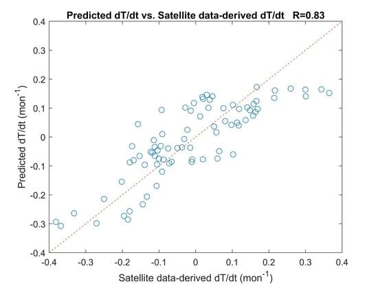
The predicted
dT/dt from Equation (7) versus satellite-derived
dT/dt data is shown in
Figure 3. The 1:1 line is also illustrated as a red dashed line. The data points of the predicted
dT/dt versus
dT/dt are close to the 1:1 line. The correlation coefficient (
R) reaches 0.83, suggesting that the equation of the WDAO model can represent the actual situation well. The coefficients in
Table 3 reveal the relative importance of the wind forcing, local temperature, and the delayed temperature. They show that
k2 has the largest absolute value (0.12), suggesting that the delayed temperature forcing is the major factor that contributes to the change of the rate of
T. The second largest is the wind forcing coefficient
β (0.057), which is approximately half of the delayed temperature and about 3 times higher than the absolute value of the coefficient of un-delayed temperature forcing (0.018). This demonstrates that, for the 1997–1998 El Nino event, the wind forcing and the delayed temperature were the major forcing factors.
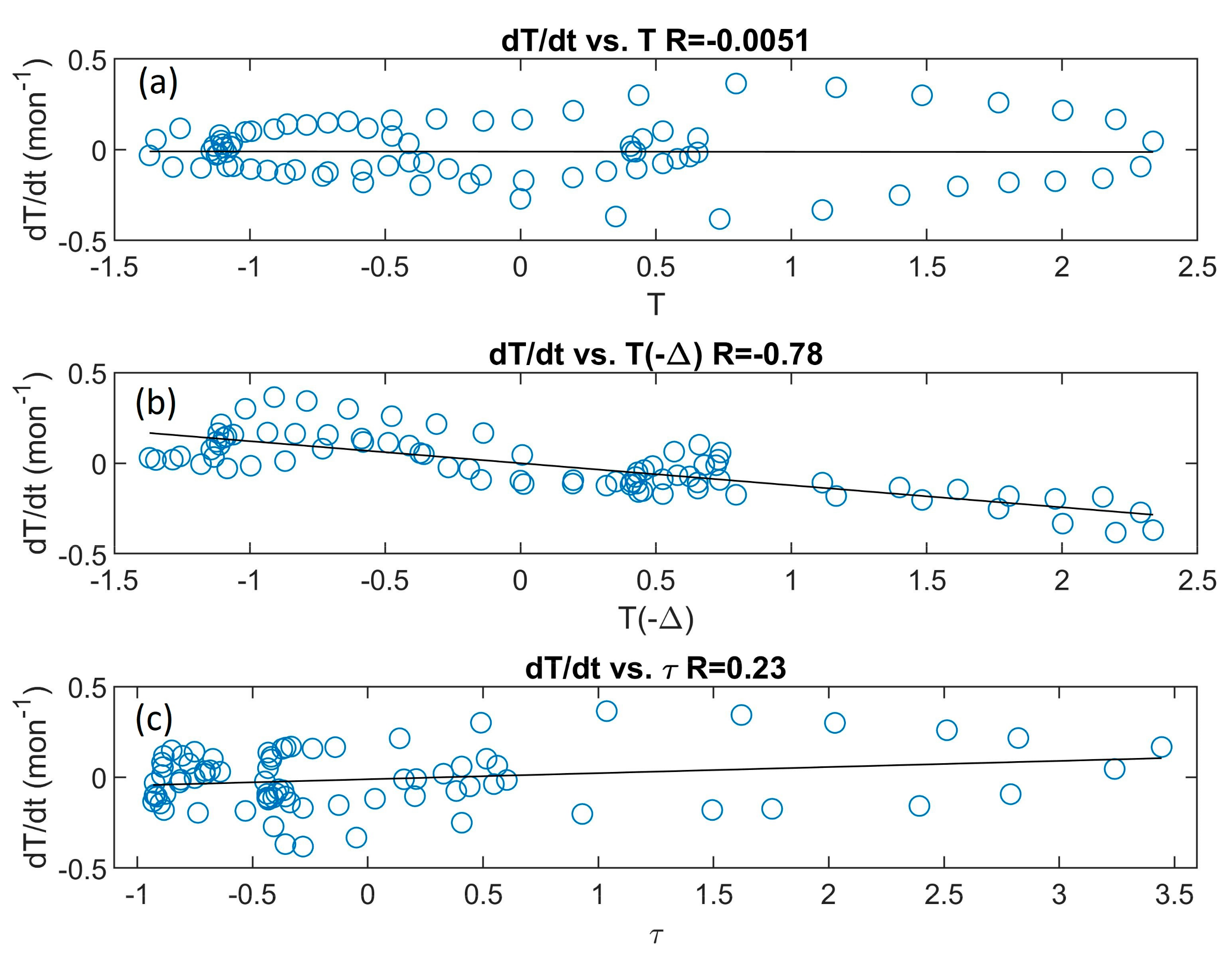
The temperature change rate in relation to different forcing parameters can be further revealed by
Figure 4, which shows
dT/dt versus
T (
Figure 4a),
dT/dt versus delayed SST (
T(-Δ)), and
dT/dt versus wind stress (
τ).
Figure 4 reveals that
dT/dt and delayed SST have the best linear relationship, with a correlation coefficient of −0.78. The correlation between the
dT/dt and the wind stress τ is 0.23, less than that seen between
dT/dt and delayed SST, but much larger than that seen between
dT/dt and un-delayed SST (−0.0051). This result suggests that delayed SST and wind forcing are the major forcing factors of SST change. The linear relations also validate the result revealed by the wind-forced delayed action oscillation analysis.
5. Discussion
The wind can be a perturbation source during a developing period of El Nino events. This can be shown by the correlation analyses and the relevant forcing term in the WDAO model. It is revealed from the WDAO equation that the wind forcing coefficient
β is positive, suggesting that wind forcing is a positive feedback of a change in the sea surface temperature; the perturbed westerly wind can lead to an increase of SST in the eastern tropical Pacific and a decrease in the western tropical Pacific [
23]. The WDAO equation also shows that
k2 is positive, indicating that the temperature delay is indeed a restoring forcing for the WDAO system. During the period between October 1995 and June 2002, the temperature delay for the restorative action was 9 months.
The study’s results show that the sea surface wind variation leads the temperature variation. It is reasonable to infer that the wind may induce a perturbation over the entire tropical region because there is no physical boundary between air masses. Therefore, the interannual variability of the atmosphere could be similar to global waves in the tropical region, which may be responsible for the interannual variability of SST.
Altimeter-derived sea level anomaly data were used for observation of equatorial ocean Kelvin and Rossby waves [
24,
25,
26,
27]. The equatorial ocean Kelvin and Rossby waves are closely related to the interannual variability of SSHA [
23]. In the ocean, SSH variability generally lags behind SST variability, reflecting the fact that equatorial SSHA lags behind SST, and that SST is more sensitive to atmospheric circulations than the equatorial ocean waves.
In this study, the strong ENSO case of 1997–1998 was studied. While the study showed the relevance of the satellite remote sensing data with the WDAO, the length of record of the coincident remote sensing observations is too short to allow us to generalize the results and conclusions to climate/decadal-scale phenomena, such as ENSO; in general, this is because the data analyzed by all data sets span only a decade. For the strong El-Nino event of 1997–1998, the results are robust. Overall, it should be emphasized that the results remain at the stage of several case-studies. It is also of interest to consider mechanisms of the El Nino Modoki cycle, such as that which occurred in 2015 and had a different impact on the Indian Ocean than regular El Nino events [
18]. Therefore, more detailed investigations must be conducted in upcoming studies with more in-situ and remote sensing data.
6. Conclusions
This study investigated the correlations of atmospheric and oceanic parameters, namely wind, sea surface temperature, and sea surface, using an EOF decomposition method. We utilized satellite observations of scatterometer-derived wind, AVHRR SST, and altimeter-derived SSHA and extracted their interannual variability to represent the variability related to ENSO. Comparisons among the EOF modes of wind, SST, and SSHA showed that the variability of the wind leads to SST and SSHA variability during the developmental stage of El Nino events. This is particularly true of the strong 1997–1998 ENSO event, which suggests that wind forcing may be an important factor influencing the ENSO system.
A WDAO system was presented that incorporates a wind forcing term in the delayed action oscillator equation. The first temporal modes of the wind and SST data in the period of October 1995 to June 2002 were used to solve the WDAO equation with a least squares method. The SST and wind stress were normalized to make the forcing terms of wind and SST comparable, so that the magnitudes of the forcing coefficients reflect their relative importance in the WDAO system. The results showed that the time delay of the wind forcing is 9 months, and the forcing coefficients for wind, delayed SST, and un-delayed SST are 0.057−0.018 and 0.12 (mon−1), respectively. The results indicate that delayed SST is the most important forcing term (with the negative value showing a restorative action), wind stress is the second most important forcing factor, and un-delayed temperature is the least important factor. The correlation between the rate of change of SST and delayed SST is 0.78, the correlation between the rate of change of SST and the wind stress is 0.23, and the correlation between the rate of change of SST and the un-delayed SST is essentially insignificant (−0.0051). The linear relationship among the rate of change of SST, wind stress, and delayed/un-delayed SST also confirms the WDAO analysis’ results, indicating that the WDAO system may better reflect the coupling of the atmosphere and the ocean for interannual variability of SST, which is closely related to the ENSO cycle.


