Article

The Climate Monitoring SAF Outgoing Longwave Radiation from AVHRR

Royal Meteorological Institute of Belgium, B-1180 Brussels, Belgium
*
Author to whom correspondence should be addressed.
Remote Sens. 2020, 12(6), 929; https://doi.org/10.3390/rs12060929
Submission received: 31 January 2020 / Revised: 3 March 2020 / Accepted: 10 March 2020 / Published: 13 March 2020
(This article belongs to the Special Issue Earth Radiation Budget)

Abstract

:
Data from the Advanced Very High Resolution Radiometer (AVHRR) have been used to create several long-duration data records of geophysical variables describing the atmosphere and land and water surfaces. In the Climate Monitoring Satellite Application Facility (CM SAF) project, AVHRR data are used to derive the Cloud, Albedo, and Radiation (CLARA) climate data records of radiation components (i.a., surface albedo) and cloud properties (i.a., cloud cover). This work describes the methodology implemented for the additional estimation of the Outgoing Longwave Radiation (OLR), an important Earth radiation budget component, that is consistent with the other CLARA variables. A first step is the estimation of the instantaneous OLR from the AVHRR observations. This is done by regressions on a large database of collocated observations between AVHRR Channel 4 (10.8 µm) and 5 (12 µm) and the OLR from the Clouds and Earth’s Radiant Energy System (CERES) instruments. We investigate the applicability of this method to the first generation of AVHRR instrument (AVHRR/1) for which no Channel 5 observation is available. A second step concerns the estimation of daily and monthly OLR from the instantaneous AVHRR overpasses. This step is especially important given the changes in the local time of the observations due to the orbital drift of the NOAA satellites. We investigate the use of OLR in the ERA5 reanalysis to estimate the diurnal variation. The developed approach proves to be valuable to model the diurnal change in OLR due to day/night time warming/cooling over clear land. Finally, the resulting monthly mean AVHRR OLR product is intercompared with the CERES monthly mean product. For a typical configuration with one morning and one afternoon AVHRR observation, the Root Mean Square (RMS) difference with CERES monthly mean OLR is about 2 Wm−2 at 1° × 1° resolution. We quantify the degradation of the OLR product when only one AVHRR instrument is available (as is the case for some periods in the 1980s) and also the improvement when more instruments are available (e.g., using METOP-A, NOAA-15, NOAA-18, and NOAA-19 in 2012). The degradation of the OLR product from AVHRR/1 instruments is also quantified, which is done by “masking” the Channel 5 observations.

Graphical Abstract

1. Introduction

The Climate Monitoring Satellite Application Facility (CM SAF) [1] has been established to provide an important contribution to the global climate monitoring. One of the main successes of this project is the generation of the Cloud, Albedo, and Radiation (CLARA) dataset based on the global observations from the Advanced Very High Resolution Radiometer (AVHRR) [2] onboard the NOAA and METOP satellites. A first edition of the CLARA dataset [3] was released in 2013, and a second one followed in 2017 [4]. CM SAF is currently developing a third edition, CLARA-A3, with a planned release at the end of 2021. Table 1 details the covered periods and the product portfolio for these three editions of the dataset.
CLARA-A3 will provide more than 40 years of data. Figure 1 shows the Equator Crossing Time (ECT) for the different NOAA and METOP polar satellites used in the Climate Data Record (CDR). The products (Table 1) are related to the description of the energy cycle in the climate system. The Top-Of-Atmosphere (TOA) Reflected Solar Flux (RSF), and Outgoing Longwave Radiation (OLR) are new products that will be included in CLARA-A3. They build on the historical CLARA cloud and radiation products to provide a consistent representation of the radiative fluxes of the Earth system. The AVHRR observations are pre-processed using a dedicated tool (PyGAC) described in detail by Devasthale et al. [5]. This tool performs in particular the calibration and homogenization of the observations, which is a necessary step toward the generation of a CDR.
The narrowband-to-broadband conversion needed for the new AVHRR-based RSF product in CLARA-A3 was discussed in Akkermans and Clerbaux [7]. The current companion paper describes the methodology developed to estimate the new OLR product and shows some preliminary validation results. In addition, the current paper discusses some important questions related to the OLR estimation from AVHRR, such as the possibility to incorporate early AVHRR instruments without Channel 5 observations. The use of state-of-the-art reanalysis is also discussed to model the diurnal cycle of the radiation, a necessary step to estimate daily and monthly mean climate products.
The users of the CLARA data records are mainly scientists performing climate studies, but there are also many other applications. The previous CLARA-A1 and CLARA-A2 releases were used in scientific studies for various purposes, e.g., (Ant)arctic surface albedo/flux studies, global/regional climate model evaluation, global/regional climate monitoring, evaluation of surface radiation climatologies and networks, climate trend studies including inter-comparison of satellite data with other observations, studies of physical processes (e.g., fluxes and evapotranspiration), new validation methods and development of algorithms, etcetera.
The main drawbacks from currently existing OLR CDRs based on broadband radiance measurements are temporal and geographical coverage: the state-of-the-art Clouds and the Earth’s Radiant Energy System (CERES [8]) products only start in 2000, while the Geostationary Earth Radiation Budget (GERB [9]) products are limited to the Meteosat field of view (longitude 0°). The need for a global, long-term OLR dataset that would fit the needs of the climate modeling and monitoring community triggered many attempts to overcome these drawbacks by relying on single-instrument narrowband data records dating back several decades. Worth noting here are the 2.5°-resolution AVHRR-based OLR CDR developed at NOAA [10,11] and the 1°-resolution CDR based on the High Resolution Infrared Radiation Sounder (HIRS) developed at the University of Maryland [12]. The CLARA-A3 OLR product aims to improve on these datasets in terms of (i) spatial resolution, i.e., unprecedented resolution of 0.25°, (ii) complementarity with other CDRs, e.g., CLARA-A3 cloud mask, and (iii) performance, e.g., bias and RMSE with respect to CERES.
The remainder of the paper is organized into three core sections and a final discussion.
Section 2 presents and discusses the estimation of the instantaneous OLR broadband flux from the brightness temperatures in the AVHRR thermal channels. The absence of Channel 5 (12 µm) for the early AVHRR instruments is quantified. The effect of surface emissivity, an important source of uncertainty in the OLR estimation, is also discussed.
Section 3 presents and discusses the estimation of the daily and monthly mean flux values from the instantaneous OLR values. This necessitates a modeling of the diurnal cycle of OLR radiation, which is especially critical given the ECT drift of the NOAA satellites (Figure 1). This work shows that accurate results can be obtained using state-of-the-art atmospheric reanalysis.
Section 4 is dedicated to the overall validation of the monthly mean OLR products with respect to the CERES monthly mean [8] products.

2. Instantaneous OLR Estimation

2.1. Problem Statement

The AVHRR instruments provide spectral observations in three thermal channels centered at 3.74 µm (Channel 3), 10.8 µm (Channel 4), and 12 µm (Channel 5). As in previous work (e.g., NOAA OLR [10,11]), Channel 3 is not considered for OLR estimation because of the strong contamination of this channel by reflected solar radiation during daytime. For this reason, Channel 3 is usually not used during daytime and is therefore replaced by observations at 1.6 µm for some instruments. Channel 4 provides measurement of the energy leaving the TOA in the atmospheric transmission window (8–12 µm), which is the main driver of the OLR variability. Channel 5 provides an additional measurement at the border of the atmospheric window, which is, when combined with Channel 4, very informative about the presence of semi-transparent high-level clouds (cirrus).
The instantaneous OLR estimation combines two challenges: (i) the spectral extrapolation needed to estimate broadband unfiltered radiation (i.e., the total thermally emitted radiation whatever is the wavelength) from narrow spectral channels and (ii) the angular extrapolation needed to estimate the hemispheric radiative flux from the directional AVHRR measurements.

2.2. OLR Regressions

In this work, spectral and hemispheric extrapolations are performed by direct regressions between the AVHRR brightness temperatures in Channels 4 and 5 and the CERES instantaneous OLR.
The regression equation has been established by selecting predictors (input variables) using a technique close to a stepwise regression. The best predictors were selected after performing an exhaustive search among various variables and using a least-squares method on the residual error. For this, the dataset was first split into two equal parts: one for the model fitting (i.e., the learning set) and one for evaluation (i.e., the test dataset). This was important to reduce the risk of “over-fitting” of the data. The selection of the best model was done in such a way to minimize the residual error on the test dataset while maintaining the number of predictors as low as possible.
We tried to maximize the use of observational satellite data to estimate the OLR. From AVHRR, the two main predictors were the brightness temperatures T 4 (K) in the 10.8 µm channel and T 5 (K) in the 12 µm channel. As a strong auto-correlation existed between these two temperatures, T 5 was not used directly, but was instead expressed as their difference ( T 5 T 4 ). This difference was a very good indicator of high semi-transparent clouds, which had a strong effect on the anisotropy of the TOA longwave radiance field [13].
To improve model performance, additional predictors were taken from the ERA5 reanalysis [14] based on their relevance for OLR estimation and their complementarity with the AVHRR observations. A first ERA5 predictor was the surface skin (radiometric) temperature T s u r f (K). This variable was important as the anisotropy of the TOA longwave radiance field was directly dependent on the temperature difference between surface and atmosphere. The higher was this difference, the more anisotropic was the radiance field at the TOA. This fact has been recognized by many authors (e.g., [15]) and was implemented in angular dependency models for LWradiation (e.g., [16]). To reduce correlation with T 4 , surface skin temperature was not used directly in the regression, but was expressed as their difference ( T 4 T s u r f ). A second predictor from the ERA5 reanalysis was the total column of water vapor T C W V (kg m−2). Water vapor has a direct effect on the radiation through absorption over an extended part of the infrared spectrum. The ERA5 variables T s u r f and T C W V were spatially and temporally interpolated to the AVHRR footprint from their native spatial (0.3°) and temporal (1 h) resolution.
Atmospheric aerosols affect the infrared spectrum by absorption and scattering of radiation, especially in some desert regions [17]. Using information about aerosol content (e.g., the aerosol optical depth product from the deep blue algorithm applied to MODIS data) in the regression was however not possible, since the AVHRR OLR CDR extended back in time until the 1980s, a period when no reliable aerosol information over land was available. The absorbing effect of aerosols on the OLR was however expected to be largely observed in the AVHRR 10.8 µm channel ( T 4 ).
Like aerosols, thin cirrus clouds would affect the TOA spectrum by absorption of infrared radiation. The effect of cirrus clouds is especially important as the semi-transparent cloud layer is often located at a very cold altitude in the troposphere (typically 8 to 14 km). In an extensive study, Lolli et al. [18] quantified the cirrus Cloud Radiative Effect (CRE), and thus the OLR decrease, to be about 2.5 Wm−2 over land, which was about 1% of the mean OLR value. This decrease of OLR due to the cirrus cloud was expected to be largely observed in T 4 . Cirrus clouds do not only affect the magnitude of the OLR through absorption, they have also a strong effect on the anisotropy of the infrared radiance field at the TOA, the so-called infrared limb-darkening. The effect on the radiance field anisotropy is explained by the rapid increase of the optical path through the cloud at increasing viewing zenith angle. The difference in brightness temperature between AVHRR Channels 4 and 5 ( T 5 T 4 ), which is one of the predictors in Equation (1), is a good indicator for the presence of thin high level clouds like cirrus. The split window technique has been used since a long time to detect cirrus clouds in AVHRR images [19].
During an exhaustive search for the best set of predictors, the four above-mentioned predictors were considered, i.e., T 4 , ( T 5 T 4 ), ( T 4 T s u r f ), and T C W V , as well as their second orders and the cross-terms. A good trade-off between regression performance and number of predictors was obtained after adding ( T 4 2 ) and ( T 4 · ( T 5 T 4 ) ). Adding more predictors in the regression had a negligible effect on the performance. Equation (1) shows the resulting regression fit with six predictors and seven coefficients ( c i ).
O L R = c 0 + c 1 · T 4 + c 2 · ( T 5 T 4 ) + c 3 · ( T 4 T s u r f ) + c 4 · T 4 2 + c 5 · T 4 · ( T 5 T 4 ) + c 6 · T C W V
The seven regression coefficients were estimated from a large database of collocated CERES OLR and AVHRR brightness temperatures. The instantaneous CERES OLR came from the Edition 4 Single Scanner Footprint (SSF) data [20]. The construction of this CERES/AVHRR database was described in Akkermans and Clerbaux [7], Section 3.1. The database contained pairs of collocated observations for NOAA-17, -18, and -19 with CERES on Terra (NOAA-17) and Aqua (NOAA-18 and -19). Given the huge number of collocated observations in this database (157.185.483), it was possible to improve the accuracy by performing dedicated regressions: (i) for the 12 calendar months, (ii) in regional boxes of 10° × 10° of latitude and longitude, and (ii) in intervals of 5° for the Viewing Zenith Angle (VZA).
The average number of observations after this stratification was about 1400 per month, regional box, and VZA interval. This was sufficient to prevent over-fitting of the seven regression coefficients ( c i ).
When Equation (1) was used to estimate the OLR corresponding to the AVHRR observations ( T 4 , T 5 ) and ancillary data ( T s u r f , T C W V ), a quadri-linear interpolation was performed according to the time of observation (to interpolate between the 12 calendar months), the latitude-longitude of the observation (to interpolate between the 10° × 10° regional boxes), and the VZA of the observation (interpolation with the 5° VZA intervals).
The first AVHRR instruments (version AVHRR/1) onboard the early NOAA satellites (TIROS-N, NOAA-6/-8/-10) did not provide Channel 5 observations. Regression Equation (1) is then modified to:
O L R = c 0 + c 1 · T 4 + c 2 · ( T 4 T s u r f ) + c 3 · T 4 2 + c 4 · T C W V
where the four regression coefficients ( c i ) are estimated from the same database of collocated AVHRR-CERES observations that was used to derive Equation (1), i.e., based on NOAA-17, -18, and -19, except that the Channel 5 brightness temperature was discarded. As expected, a slightly higher uncertainty was obtained. The RMS error increased from 4.75 Wm−2 (i.e., 2.2% on the 216 Wm−2 average OLR) when Equation (1) was used to 5.86 Wm−2 (2.7%) with Equation (2).

2.3. Results

Figure 2 shows the spatial distribution of the regression error’s RMS, in boxes of 1° × 1° latitude-longitude (all months and all VZAs together). In each box, this RMSE was calculated by collecting all instantaneous OLR observations (CERES SSF) and corresponding OLR estimations (AVHRR-derived) and computing the root mean square over all their differences. The spatial pattern could be explained by cloudiness. Higher error was associated with high level clouds, reflecting the combination of increased AVHRR-CERES matching error and, in the case of cirrus, increased anisotropy. Lower error was observed over anticyclonic regions, characterized by mostly low level uniform cloud fields, and over polar regions, where OLR magnitude and variability were much lower. The results shown in Figure 2a (top panel) were obtained using Equation (1) (when Channels 4 and 5 were available) while those shown in Figure 2b (bottom panel) used Equation (2) (Channel 5 was not available). With Equation (1), the RMS error of the OLR regression typically ranged between 2 and 8 Wm−2 (about 1 to 3% of the mean OLR value). There was a significant latitudinal dependency, which was directly related to the latitudinal variation of the OLR with decreasing values from the Equator to the poles. For a same latitude band, a higher RMSE was generally observed over land compared to ocean. This was explained by the higher variability of the land surface temperature (due to daytime warming of the surface), higher variability of the land surface emissivity, and also, the higher convective activity. The histograms of the regional RMS difference (Figure 2, right) showed similar patterns for Equation (1) (black) and Equation (2) (red), but with slightly higher RMS error for Equation (2).
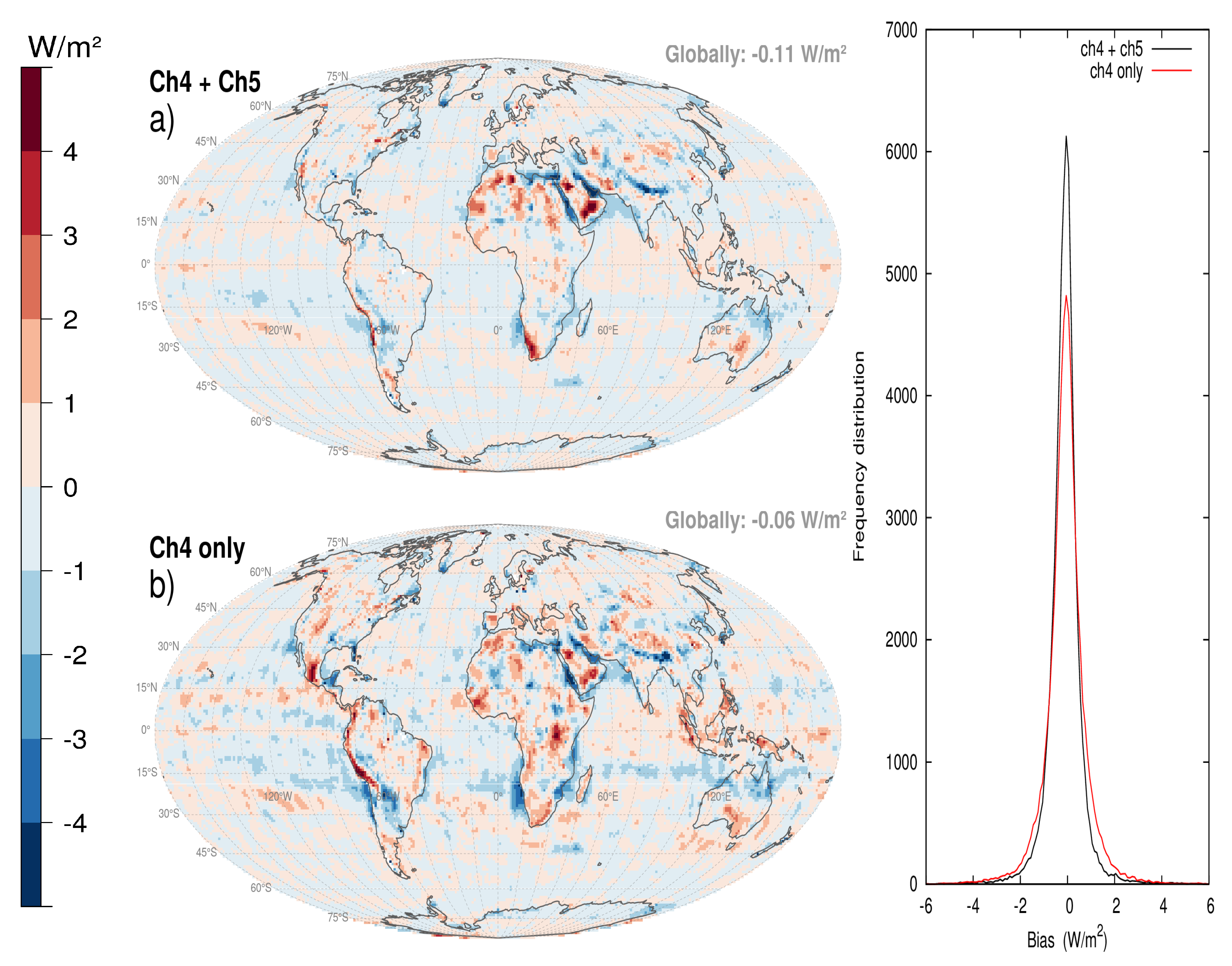
Figure 3 shows the spatial distribution of the regression error’s bias, in boxes of 1° × 1° latitude-longitude (all months and all VZAs together). This was done similarly to the RMSE, with bias defined as AVHRR OLR minus CERES SSF OLR. The histogram of the regional bias (Figure 3, right) showed a slightly higher dispersion with Equation (2) compared to Equation (1). The bias remained in general small, with absolute biases mostly lower than 0.5 Wm−2. However, significant negative biases were observed over the Red and Persian seas and positive biases over some desert regions. Those biases could be explained by the mixture of water and sandy surfaces in the 10° × 10° boxes used for the regressions. The variability of the surface thermal emissivity affected mostly the λ < 10 µm spectral range and therefore had more impact on the (broadband) OLR than on the AVHRR with channels at 10.5 and 12 µm; this explained the overestimation over land and the underestimation over ocean in those specific coast-desert mixture boxes.
Table 2 provides some statistics about the regional 1° × 1° values of the RMS error and bias, all months and VZA together.
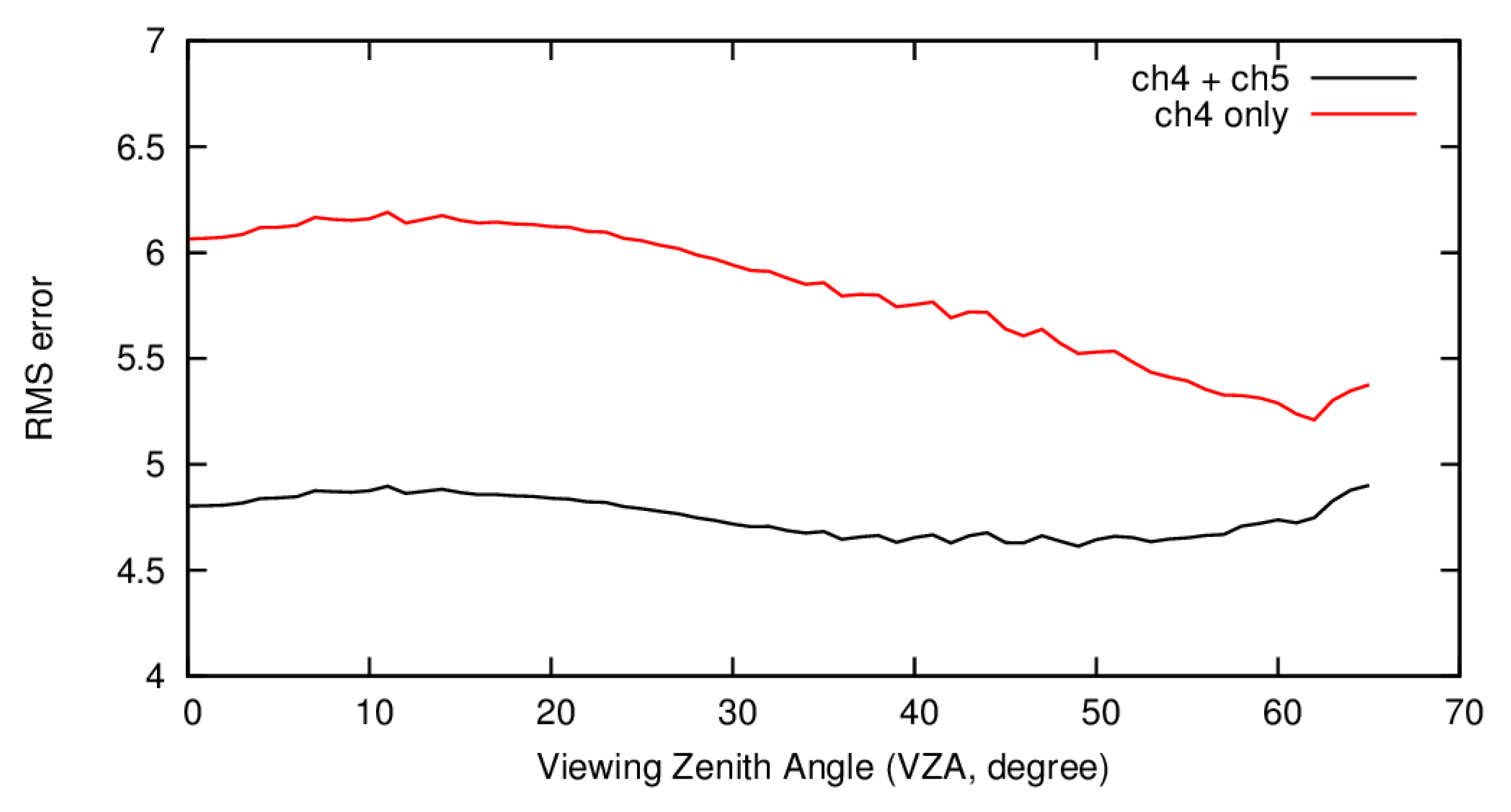
Figure 4 shows the variation of the RMS error as a function of VZA, using Equations (1) (black) and 2 (red). Overall, the VZA dependency was limited. For Equation (2), the RMS error decreased with VZA, which could be explained by the growing CERES footprint size and hence decreasing variability. The almost flat curve observed when using Equation (1) showed nevertheless a slight improvement for VZAs between 40–50°. This behavior could be explained by the fact that the observations at these VZAs were good approximations for the hemispherical flux [13].
Table 3 provides some statistics for Equations (1) and (2), per satellite separately. The biases remained moderate, an indication of a good intercalibration of the thermal channels for the three satellites and a good consistency between the CERES instruments on Terra and Aqua. However, Equation (1) applied to NOAA-19 showed a negative bias (underestimation of the OLR) of 0.77 Wm−2, which was about 0.35% of the average OLR. Concerning the RMS error, NOAA-17 showed slightly better results than NOAA-18 and -19. This could indicate better performance of the AVHRR instrument on this satellite (e.g., less noise), but was more likely related to the fact that NOAA-17 is a morning satellite, when the estimation of the instantaneous OLR is less affected by the daytime warming of the land surface.
The bias and RMS differences between the AVHRR-based and CERES OLR discussed in this section were affected by the collocation methodology in space and in time. The OLR accuracy is further discussed in Section 4.

3. Daily and Monthly Mean OLR

3.1. Problem Statement

To make them useful for climate studies, AVHRR-derived instantaneous OLR observations should be converted to daily and monthly means, as well as be rectified onto a fixed grid (0.25° × 0.25° for CLARA-A3). The spatial regridding procedure consisted of a simple averaging of AVHRR pixel falling in their corresponding 0.25° × 0.25° grid box, based on the AVHRR pixel center coordinates, and is not further discussed in this paper. On the other hand, the temporal processing was more challenging since, over land, the OLR often exhibited a strong diurnal variation due to daytime surface warming. Given the drifts in ECT of the NOAA satellites, this conversion must be performed with care to avoid introducing spurious trends and discrepancies at satellite switches in the resulting CDR (see for example [21]).
In the CERES products, the diurnal cycle was taken into account using data from geostationary satellites [22]. However, this approach was hardly implemented for CDRs covering the 1980s and 1990s due to degraded geostationary data quality and completeness. The HIRS OLR CDR used geostationary infrared observations from the NOAA GridSat [23] as described by Schreck et al. [24]. GridSat however did not provide data before 1981 and also had a gap over the Indian ocean in the 1980s and 1990s. In this work, an alternative approach was investigated, using information about the OLR diurnal cycle from ERA5 reanalysis [14], which provided full temporal and spatial coverage.

3.2. Method

In ERA5, the TOA reflected solar flux and emitted thermal fluxes were simulated using ecRad [25]. The ERA5 fluxes were provided as one hour averages at a spatial resolution of 31 km. This spatial resolution was close to the CLARA-A3 grid of 0.25° × 0.25°.
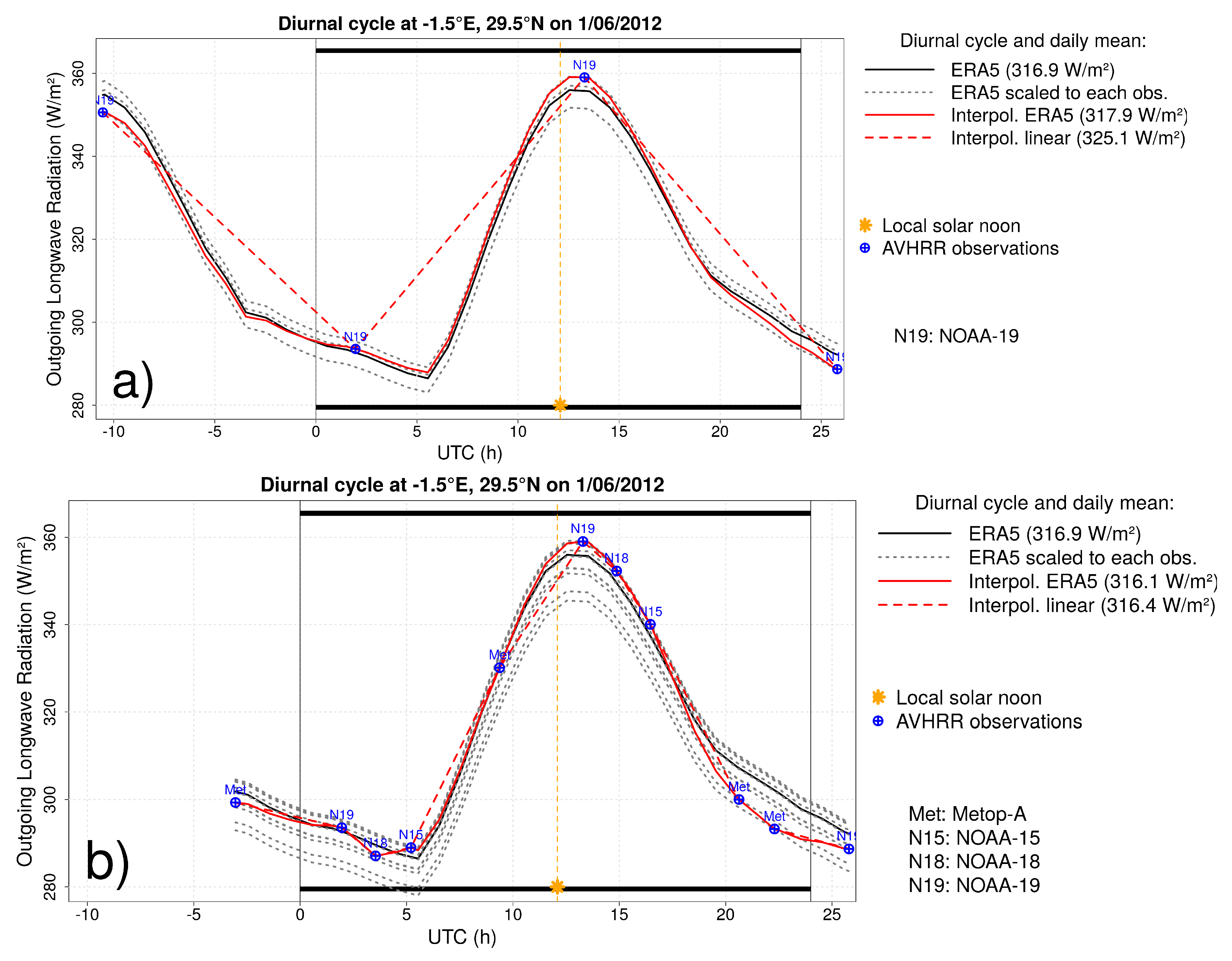
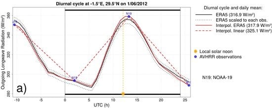
Figure 5a shows an illustrative OLR diurnal cycle from ERA5 (black curve) together with the AVHRR observations from NOAA-19 acquired during this time period (blue dots). For each AVHRR observation, a factor was determined between the ERA5 and the observed OLR, which was used to scale the entire ERA5 diurnal cycle (dotted grey curves). These scaled diurnal cycles were then temporally interpolated (inversely weighted to their temporal difference) so that the cycle passed exactly through all observations (red curve). This was only done for observations over land that were considered “clear-sky” by both AVHRR and ERA5 (as was the case for all observations in Figure 5); for all other cases (i.e., ocean or cloudy), the observations were linearly interpolated (dashed red curve). The daily mean, and later the monthly mean, could then be estimated by averaging the interpolated diurnal cycle (dashed/solid red curves) over the entire day, i.e., 0–24 h UTC. In this example, the linear interpolation of observations resulted in a daily mean of 325.1 Wm−2 (dashed red curve), while the ERA5-scaling interpolation significantly decreased the daily mean by 7.2 Wm−2 to 317.9 Wm−2 (solid red curve).
The method could be applied, and a daily mean value could be estimated, as long as there was at least one observation during that day. Obviously, more observations spread over the day made the resulting daily mean product less sensitive to the representation of the OLR in the reanalysis: this is shown in Figure 5b, for which eight daily observations, from four different satellites, were used.
Finally, the monthly mean was obtained by simple averaging of the daily values.

3.3. Results

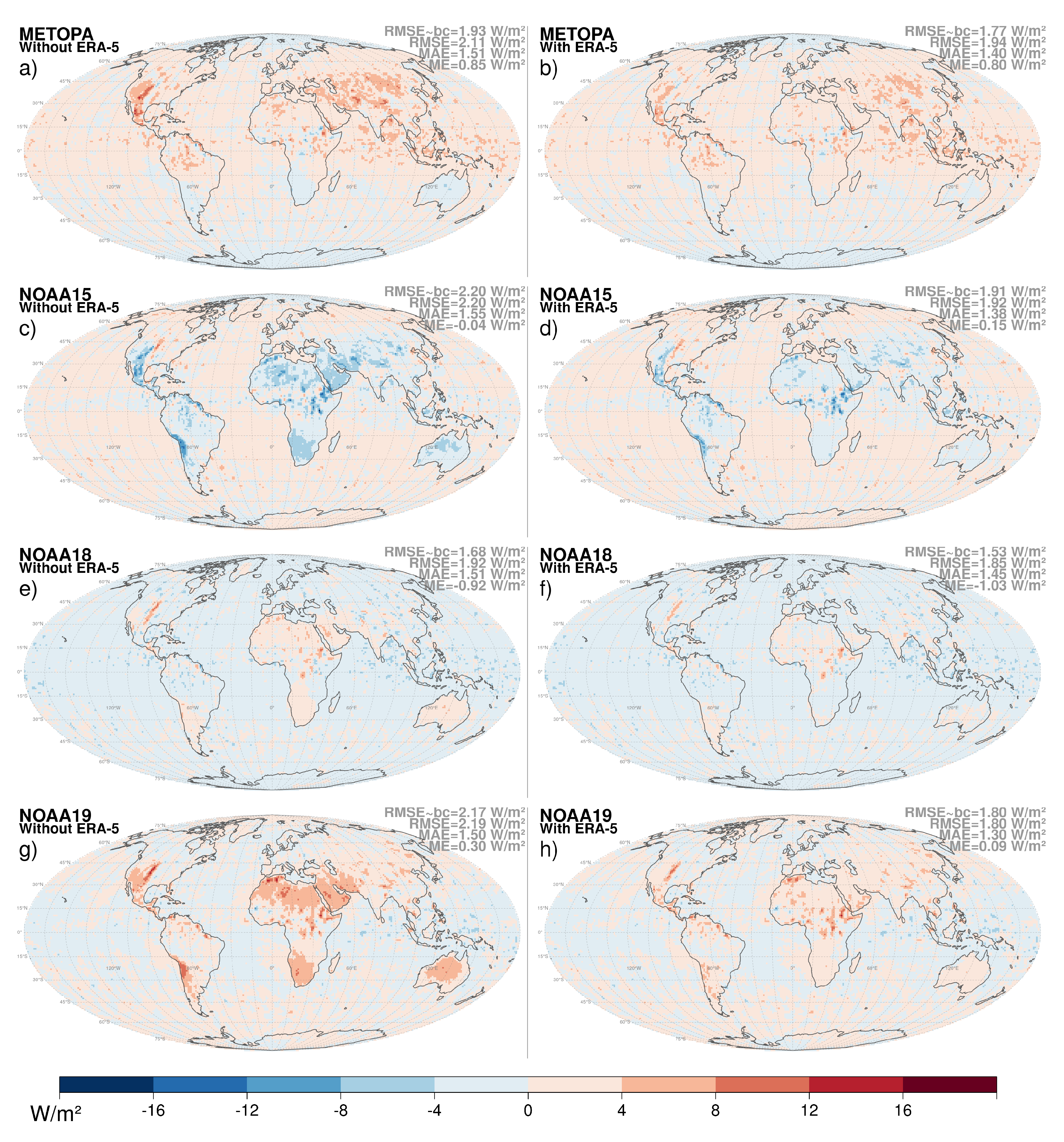
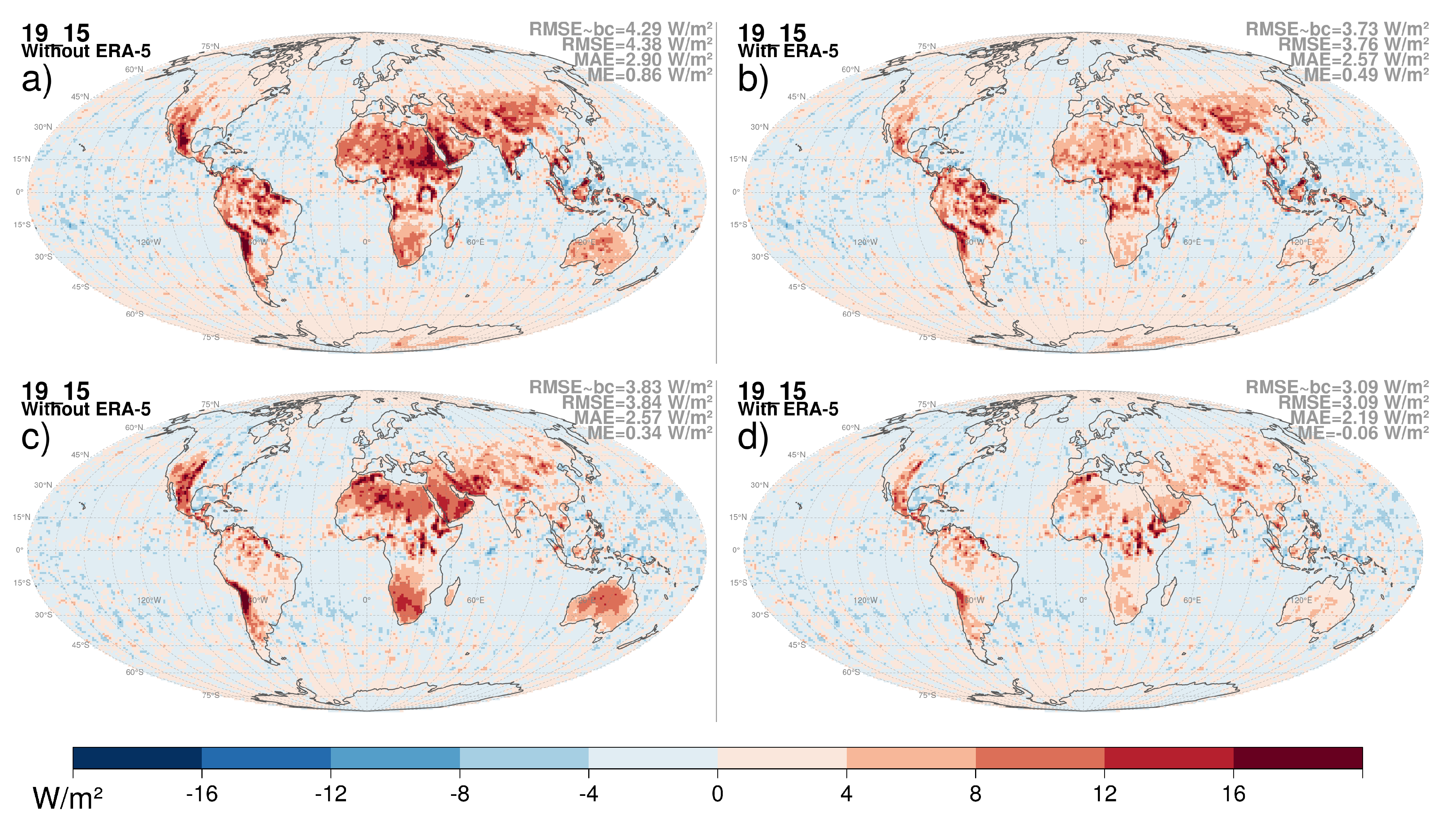
To evaluate the use of ERA5 to model the diurnal cycle, the monthly mean OLR products were computed separately for the four satellites available in April and June 2012 (METOP-A, NOAA-15, NOAA-18, NOAA-19) and compared with the monthly mean OLR value obtained when using all four satellites together, hereafter referred to as “reference monthly mean OLR”. If the diurnal cycle was correctly modeled in the processing, the monthly mean map for each individual satellite should closely agree with the reference.
Figure 6 shows the difference with the reference monthly mean OLR when the diurnal cycle was modeled by linear temporal interpolation (left) and when ERA5 was used over cloud-free land (right) for the four satellites separately. This figure was for June 2012, but similar results were obtained for April 2012 (figures not shown). Significant improvements were observed over land, especially for NOAA-15 (ECT ~17 UTC) and NOAA-19 (ECT ~13:30 UTC). On average, over the four satellites, the RMS difference over land w.r.t. the reference decreased from 2.4 Wm−2 (with linear temporal interpolation) to 2.0 Wm−2 (with ERA5-scaling interpolation). This result seemed to be a rather limited improvement, but over most of the deserts, it was significant.
Figure 7 shows the difference between the NOAA-19 and the NOAA-15 monthly mean OLR without (left) and with ERA5 (right) for April and June 2012. These satellites were selected as they produced the strongest overestimation (NOAA-19) and underestimation (NOAA-15) of the daily mean OLR when using linear temporal interpolation. This method, where the monthly mean calculated from one satellite was compared with the monthly mean calculated from another satellite, followed Doelling et al. [22] (2013). Similar to Figure 6, low differences indicated a good modeling of the diurnal cycle. The added value of ERA5 manifested itself in many clear land regions.

4. Overall Validation with Respect to CERES SYN1deg

In Section 2, the instantaneous OLR accuracy was estimated to be of the order of 4.8 Wm−2. However, this number could be affected by the AVHRR–CERES matching procedure. Furthermore, part of the error was expected to be reduced by averaging to a monthly mean. In Section 3, the additional error due to the diurnal cycle modeling was estimated to be about 2 Wm−2, but also here, the accuracy was strongly dependent on the satellites available and their ECTs. For this reason, intercomparison with the monthly mean product from CERES Synoptic 1° latitude 1° longitude gridded (SYN1deg [22]) was informative for the overall performances of the processing.
This evaluation was performed for April and June 2012, under different selections of input satellites. In a first configuration, all the satellites available (METOP-A, NOAA-15, NOAA-18, NOAA-19) were considered, providing up to eight observations per day. With this configuration, the error due to the diurnal cycle modeling was minimized. Figure 8 shows the monthly mean OLR difference with CERES SYN1deg. On average for April and June 2012, the RMS of the difference was about 2.0 Wm−2, which corresponded to 0.8% of the mean OLR (240 Wm−2). An overall negative bias of about −1.0 Wm−2 was observed, which was 0.4% of the average OLR. The bias-corrected RMS error (RMSE-bc) was about −1.7 Wm−2.
In a second configuration, only METOP-A and NOAA-19 were used in the processing (Figure 9). The results with this configuration should be representative for most of the months in the CLARA-A3 data record, which had only one morning and one afternoon satellite (Figure 1). Discarding NOAA-15 and NOAA-18 had a favorable effect on the bias, which was reduced from −1.0 Wm−2 to −0.6 Wm−2. As expected however, the bias-corrected RMSE increased from about 1.7 Wm−2 (four satellites) to about 2 Wm−2.
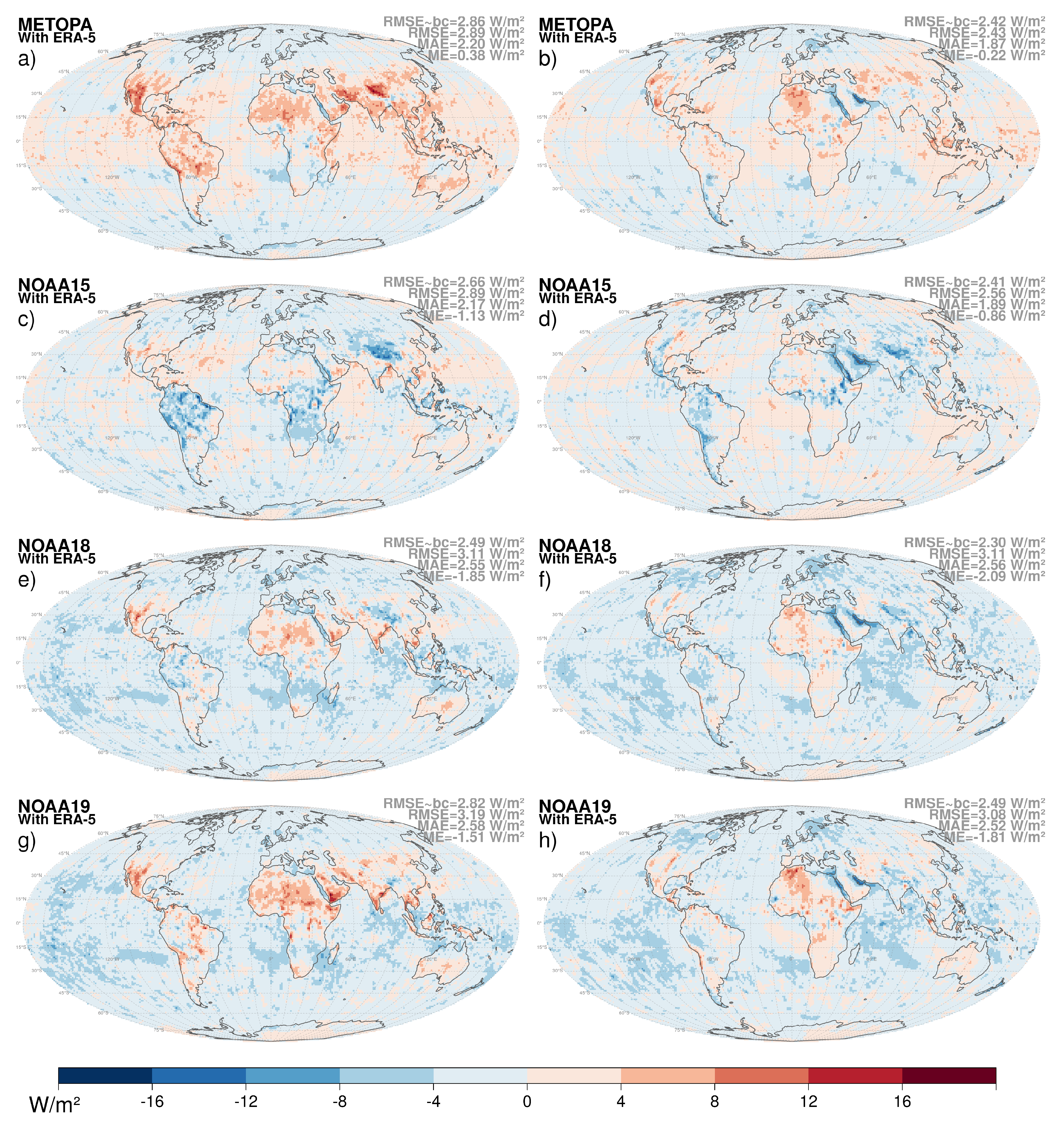
Figure 10 shows the evaluation performed using a single satellite in the processing (METOP-A, NOAA-15, NOAA-18, and NOAA-19) separately. This configuration was representative of some particular periods in the AVHRR record (gaps due to instrument absence, gaps due to instrument failure, unusable observations in sunglint conditions, etc.). With only one satellite as input, the bias-corrected RMSE lied between 2.3 Wm−2 and 2.9 Wm−2, which was slightly worse compared to the results with multiple satellites (2 Wm−2 with two satellites and 1.7 Wm−2 with four satellites). Although they had different ECT, there was no significant difference of RMSE-bc between the different satellites considered in Figure 10.
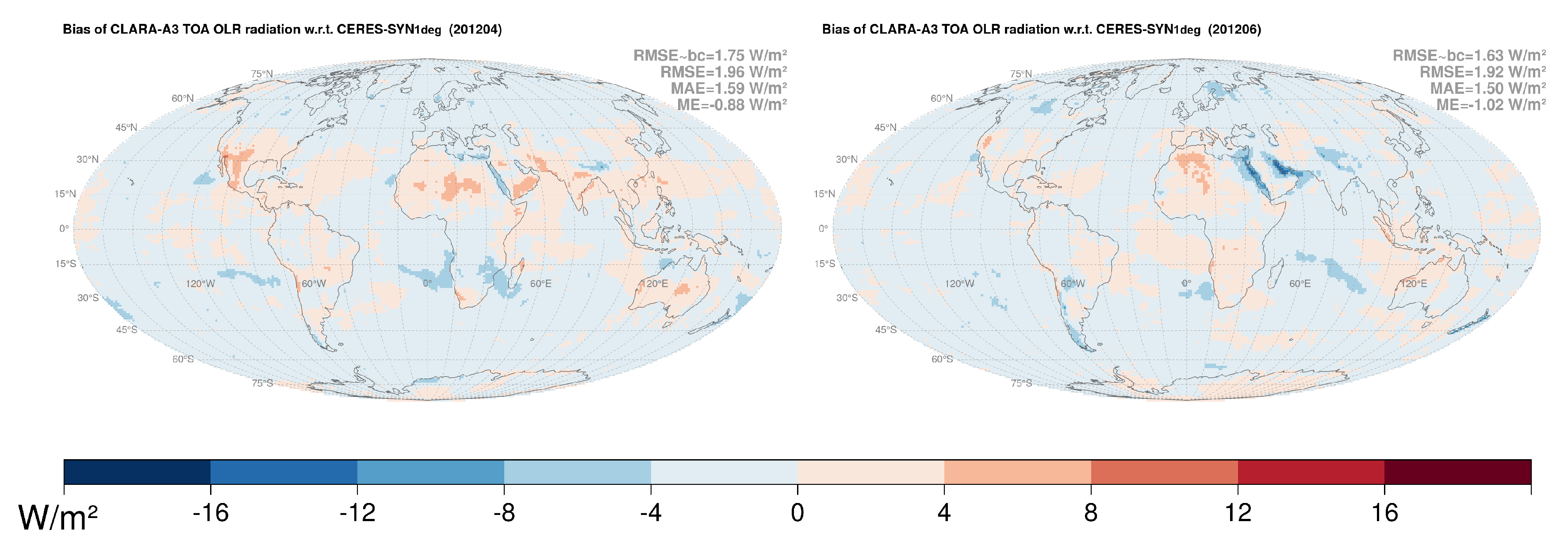
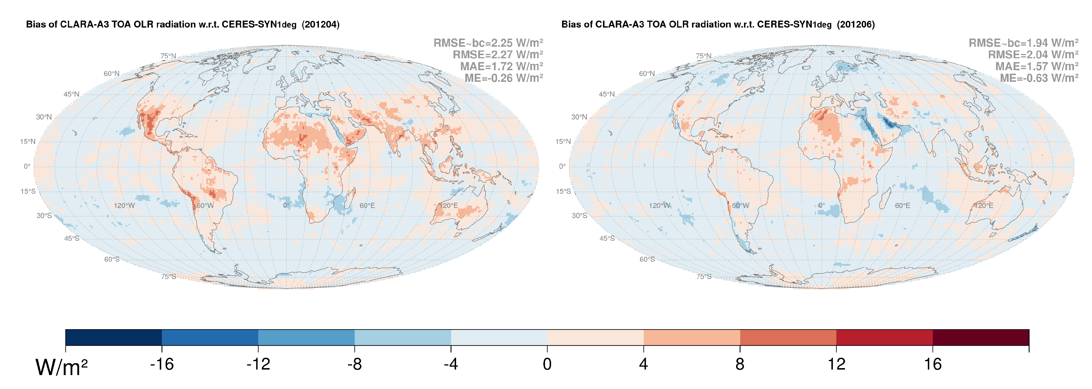
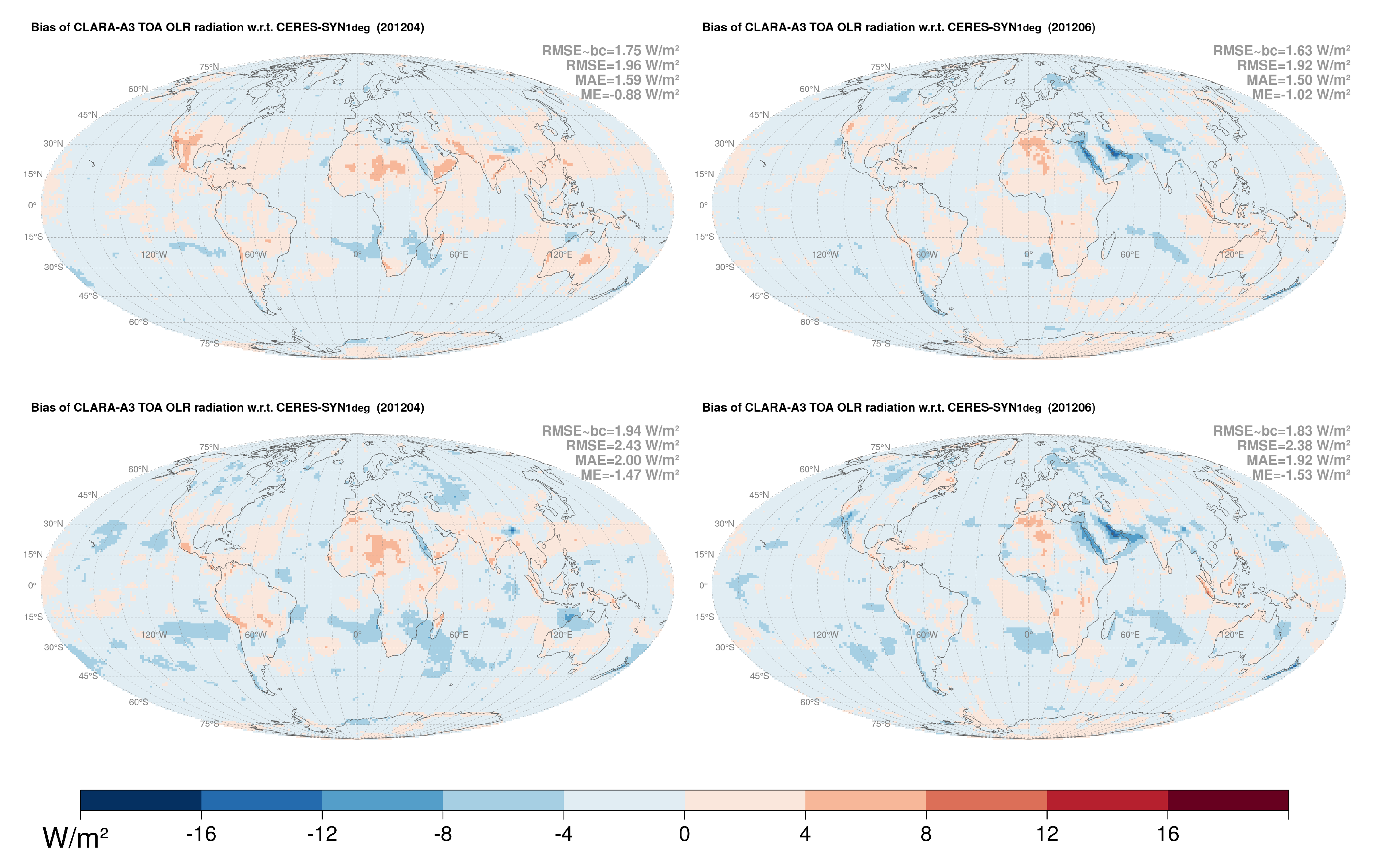
Finally, Figure 11 shows comparisons with CERES SYN1deg when the OLR was estimated with Equation (2), i.e., when the AVHRR/1 instrument was used, which did not provide Channel 5 observations. To ease the comparison, the results with both Channels 4 and 5 are also shown (top panels). When Channel 5 was not available (bottom panels), the bias-corrected RMS difference of the monthly mean increased from about 1.7 Wm−2 to about 1.9 Wm−2.

5. Summary

This paper described and discussed the method implemented by the CM SAF to estimate global OLR from the AVHRR observations. This new OLR product will be published as part of CLARA-A3 and will provide consistency with the other cloud and radiation products in CLARA. The data also had strong complementarity with the NASA CERES (extension in the past) and NOAA HIRS OLR data records (better spatial resolution, wider swath).
Instantaneous OLR was first estimated using regressions between the AVHRR Channel 4 and 5 brightness temperatures and CERES SSF OLR. A particular focus was put on the applicability of the method to the early AVHRR/1 instrument (without Channel 5 at 12 µm) so that the dataset could be extended back in time until the end of the 1970s. The developed regressions showed limited bias (|bias| < 1 Wm−2) and good accuracy (RMSE < 5 Wm−2) concerning instantaneous OLR at a 1° × 1° spatial resolution.
From the instantaneous OLR, the daily and monthly mean fluxes were estimated using an innovative method that exploited the newly released ERA5 reanalysis. Significant improvement in the Level-3 processing was observed over clear land surface. This indicated that the diurnal cycle of land surface warming was well represented in the reanalysis. Over ocean and in convective regions, there was no improvement with regard to a standard linear temporal interpolation.
Finally, overall evaluation of the monthly OLR products was performed with respect to CERES SYN1deg. The bias-corrected RMS difference in OLR was about 2 Wm−2 when one morning and one afternoon satellite were available. This 2 Wm−2 RMS difference with CERES SYN1deg was much better than the operational AVHRR OLR of NOAA (RMSE-bc of 6.2 Wm−2 at 5° × 5° resolution) and slightly better than the NOAA HIRS OLR dataset (RMSE-bc of 2.7 Wm−2). Although a part of the RMSE could be attributed to the CERES product, the accuracy was likely not compliant with the GCOS OLR accuracy requirements of 1 Wm−2 [26], stressing the need for additional improvement of the product. The intercomparison with CERES showed that, as expected, the number of available AVHRR observations had a direct impact on the accuracy of the monthly OLR. When one satellite was available, the RMSE increased to 2.5 Wm−2, while it decreased to 1.7 Wm−2 when four satellites were available. For the AVHRR/1 instrument, the RMS error increased from 2.0 Wm−2 to 2.4 Wm−2 due to the absence of Channel 5 observations.
Some important questions remain to be addressed when the full dataset will be processed, in particular concerning the stability of the record. Stability could be affected by instrument calibration, a difference in spectral channels, and drift in ECT. The variable number of available satellites could also impact the stability. This work also indicated that accounting for surface emissivity could reduce the biases in some regions having a strong spatial gradient of emissivity like coastal regions in desert areas. Investigations in this direction are foreseen in view of the subsequent version of the CDR.

Author Contributions

Conceptualization, methodology, supervision, analysis, and writing, original draft: N.C.; data curation, analysis, validation, and visualization: T.A.; reviewing and editing: T.A., J.M., A.V.B., W.M., and C.A.; resources and software: J.M. and E.B. All authors have read and agreed to the published version of the manuscript.

Funding

This work was funded by the Climate Monitoring Satellite Application Facility (CM SAF) of EUMETSAT.

Acknowledgments

The authors are grateful to the Atmospheric Science Data Center at NASA Langley Research Center for providing the CERES data used in this work.

Conflicts of Interest

The authors declare no conflict of interest.

Abbreviations

The following abbreviations are used in this manuscript:
ADMAngular Dependency Model
AVHRRAdvanced Very High Resolution Radiometer
Ch4, Ch5Channel 4, Channel 5
CDRClimate Data Record
CERESClouds and the Earth’s Radiant Energy System (instrument and mission)
CLARACM SAF cLoud, Albedo and Radiation dataset from AVHRR data
CMSAFClimate Monitoring Satellite Application Facility
ECTEquatorial Crossing Time
ERBEarth Radiation Budget (instrument and mission)
ERBEEarth Radiation Budget Experiment (instrument and mission)
FCDRFundamental Climate Data Record
FMFlight Model
GACGlobal Area Coverage
GCOSGlobal Observing System for Climate
GERBGeostationary Earth Radiation Budget (instrument and mission)
GOESGeostationary Operational Environmental Satellite
IGBPInternational Geosphere-Biosphere Programme
LSTLocal Solar Time
MODISModerate Resolution Imaging Spectroradiometer
MSGMeteosat Second Generation
MVIRIMeteosat Visible and Infrared Imager
NOAA-XNational Oceanic and Atmospheric Administration, Satellite X
OLROutgoing Longwave Radiation
RMSERoot Mean Square Error
RMSE-bcBias-corrected RMSE
RSFReflected Solar Flux
SSFSingle Scanner Footprint
SYN1degSynoptic 1° latitude 1° longitude gridded
TOATop Of Atmosphere
VZAViewing zenith angle

References

  1. Schulz, J.; Albert, P.; Behr, H.D.; Caprion, D.; Deneke, H.; Dewitte, S.; Durr, B.; Fuchs, P.; Gratzki, A.; Hechler, P.; et al. Operational climate monitoring from space: The EUMETSAT Satellite Application Facility on Climate Monitoring (CM-SAF). Atmos. Chem. Phys. 2009, 9, 1687–1709. [Google Scholar] [CrossRef] [Green Version]
  2. Cracknell, A.P. Advanced Very High Resolution Radiometer AVHRR; Taylor and Francis: London, UK, 1997. [Google Scholar]
  3. Karlsson, K.G.; Riihelä, A.; Müller, R.; Meirink, J.; Sedlar, J.; Stengel, M.; Lockhoff, M.; Trentmann, J.; Kaspar, F.; Hollmann, R.; et al. CLARA-A1: The CM SAF cloud, albedo and radiation dataset from 28 yr of global AVHRR data. Atmos. Chem. Phys. Discuss. 2013, 13, 935–982. [Google Scholar] [CrossRef] [Green Version]
  4. Karlsson, K.G.; Anttila, K.; Trentmann, J.; Stengel, M.; Meirink, J.F.; Devasthale, A.; Hanschmann, T.; Kothe, S.; Jaaskelainen, E.; Sedlar, J.; et al. CLARA-A2: The second edition of the CM SAF cloud and radiation data record from 34 years of global AVHRR data. Atmos. Chem. Phys. 2017, 17, 5809–5828. [Google Scholar] [CrossRef] [Green Version]
  5. Devasthale, A.; Raspaud, M.; Schlundt, C.; Hanschmann, T.; Finkensieper, S.; Dybbroe, A.; Hörnquist, S.; Håkansson, N.; Stengel, M.; Karlsson, K. PyGAC: An open-source, community-driven Python interface to preprocess more than 30-year AVHRR Global Area Coverage (GAC) data. GSICS Q. Newsl. 2017, 11, 3–5. [Google Scholar]
  6. Hollman, R.; Schlundt, C.; Finkensieper, S.; Raspaud, M.; Karlsson, K.G.; Stengel, M. ESA Cloud cci: Technical Report on AVHRR GAC FCDR Generation. Technical Report Issue 1, Revision 0, ESA Cloud cci. 2017. Available online: http://www.esa-cloud-cci.org/?q=documentation (accessed on 31 January 2020).
  7. Akkermans, T.; Clerbaux, N. Narrowband-to-Broadband Conversions for Top-of-Atmosphere Reflectance from the Advanced Very High Resolution Radiometer (AVHRR). Remote Sens. 2020, 12, 305. [Google Scholar] [CrossRef] [Green Version]
  8. Wielicki, B.A.; Barkstrom, B.R.; Harrison, E.F.; Lee, R.B., III; Smith, G.L.; Cooper, J.E. Clouds and the Earth’s Radiant Energy System (CERES): An earth observing system experiment. Bull. Am. Meteorol. Soc. 1996, 77, 853–868. [Google Scholar] [CrossRef] [Green Version]
  9. Harries, J.E.; Russell, J.; Hanafin, J.; Brindley, H.; Futyan, J.; Rufus, J.; Kellock, S.; Matthews, G.; Wrigley, R.; Last, A.; et al. The geostationary earth radiation budget project. Bull. Am. Meteorol. Soc. 2005, 86, 945–960. [Google Scholar] [CrossRef] [Green Version]
  10. Liebmann, B.; Smith, C.A. Description of a complete (interpolated) outgoing longwave radiation dataset. Bull. Am. Meteorol. Soc. 1996, 77, 1275–1277. [Google Scholar]
  11. NOAA Interpolated Outgoing Longwave Radiation (OLR). National Oceanic and Atmospheric Administration. Available online: https://www.esrl.noaa.gov/psd/data/gridded/data.interp_OLR.html (accessed on 30 January 2020).
  12. Lee, H.T.; Gruber, A.; Ellingson, R.G.; Laszlo, I. Development of the HIRS outgoing longwave radiation climate dataset. J. Atmos. Ocean. Technol. 2007, 24, 2029–2047. [Google Scholar] [CrossRef] [Green Version]
  13. Clerbaux, N.; Dewitte, S.; Gonzalez, L.; Bertrand, C.; Nicula, B.; Ipe, A. Outgoing longwave flux estimation: Improvement of angular modelling using spectral information. Remote Sens. Environ. 2003, 85, 389–395. [Google Scholar] [CrossRef]
  14. Hersbach, H. The ERA5 Atmospheric Reanalysis. In AGU Fall Meeting Abstracts; American Geophysical Union: Washington, DC, USA, 2016. [Google Scholar]
  15. Otterman, J.; Starr, D.; Brakke, T.; Davies, R.; Jacobowitz, H.; Mehta, A.; Cheruy, F.; Prabhakara, C. Modeling zenith-angle dependence of outgoing longwave radiation: Implication for flux measurements. Remote Sens. Environ. 1997, 62, 90–100. [Google Scholar] [CrossRef]
  16. Loeb, N.G.; Manalo-Smith, N.; Kato, S.; Miller, W.F.; Gupta, S.K.; Minnis, P.; Wielicki, B.A. Angular distribution models for top-of-atmosphere radiative flux estimation from the Clouds and the Earth’s Radiant Energy System instrument on the Tropical Rainfall Measuring Mission satellite. Part I: Methodology. J. Appl. Meteorol. 2003, 42, 240–265. [Google Scholar] [CrossRef]
  17. Di Biagio, C.; Boucher, H.; Caquineau, S.; Chevaillier, S.; Cuesta, J.; Formenti, P. Variability of the infrared complex refractive index of African mineral dust: Experimental estimation and implications for radiative transfer and satellite remote sensing. Atmos. Chem. Phys. Discuss. Eur. Geosci. Union 2014, 14, 11093–11116. [Google Scholar]
  18. Lolli, S.; Campbell, J.R.; Lewis, J.R.; Gu, Y.; Marquis, J.W.; Chew, B.N.; Liew, S.C.; Salinas, S.V.; Welton, E.J. Daytime top-of-the-atmosphere cirrus cloud radiative forcing properties at Singapore. J. Appl. Meteorol. Climatol. 2017, 56, 1249–1257. [Google Scholar] [CrossRef] [Green Version]
  19. Inoue, T. A cloud type classification with NOAA 7 split-window measurements. J. Geophys. Res. Atmos. 1987, 92, 3991–4000. [Google Scholar] [CrossRef]
  20. Geier, E.; Green, R.; Kratz, D.; Minnis, P.; Miller, W.; Nolan, S.; Franklin, C. CERES Data Management System: Single Satellite Footprint TOA/surface Fluxes and Clouds (SSF) Collection Document; Release 2, Version 1, 212pp. and Appendixes; NASA Langley Res. Cent.: Hampton, VA, USA, 2003. Available online: http://asd-www.larc.nasa.gov/ceres/collect_guide/SSF_CG.pdf (accessed on 30 January 2020).
  21. Waliser, D.E.; Zhou, W. Removing satellite equatorial crossing time biases from the OLR and HRC datasets. J. Clim. 1997, 10, 2125–2146. [Google Scholar] [CrossRef]
  22. Doelling, D.R.; Loeb, N.G.; Keyes, D.F.; Nordeen, M.L.; Morstad, D.; Nguyen, C.; Wielicki, B.A.; Young, D.F.; Sun, M. Geostationary enhanced temporal interpolation for CERES flux products. J. Atmos. Ocean. Technol. 2013, 30, 1072–1090. [Google Scholar] [CrossRef]
  23. Knapp, K.R.; Ansari, S.; Bain, C.L.; Bourassa, M.A.; Dickinson, M.J.; Funk, C.; Helms, C.N.; Hennon, C.C.; Holmes, C.D.; Huffman, G.J.; et al. Globally gridded satellite observations for climate studies. Bull. Am. Meteorol. Soc. 2011, 92, 893–907. [Google Scholar] [CrossRef]
  24. Schreck, C.J.; Lee, H.T.; Knapp, K.R. HIRS outgoing longwave radiation—Daily climate data record: Application toward identifying tropical subseasonal variability. Remote Sens. 2018, 10, 1325. [Google Scholar] [CrossRef] [Green Version]
  25. Hogan, R.J.; Bozzo, A. A flexible and efficient radiation scheme for the ECMWF model. J. Adv. Model. Earth Syst. 2018, 10, 1990–2008. [Google Scholar] [CrossRef] [Green Version]
  26. GCOS. Systematic Observation Requirements for Satellite-Based Products for Climate (2011 Update): Supplemental Details to the Satellite-Based Component of the “Implementation Plan for the Global Observing System for Climate in Support of the UNFCCC”. Reference Document GCOS-154, WMO. 2011. Available online: www.wmo.int (accessed on 30 January 2020).
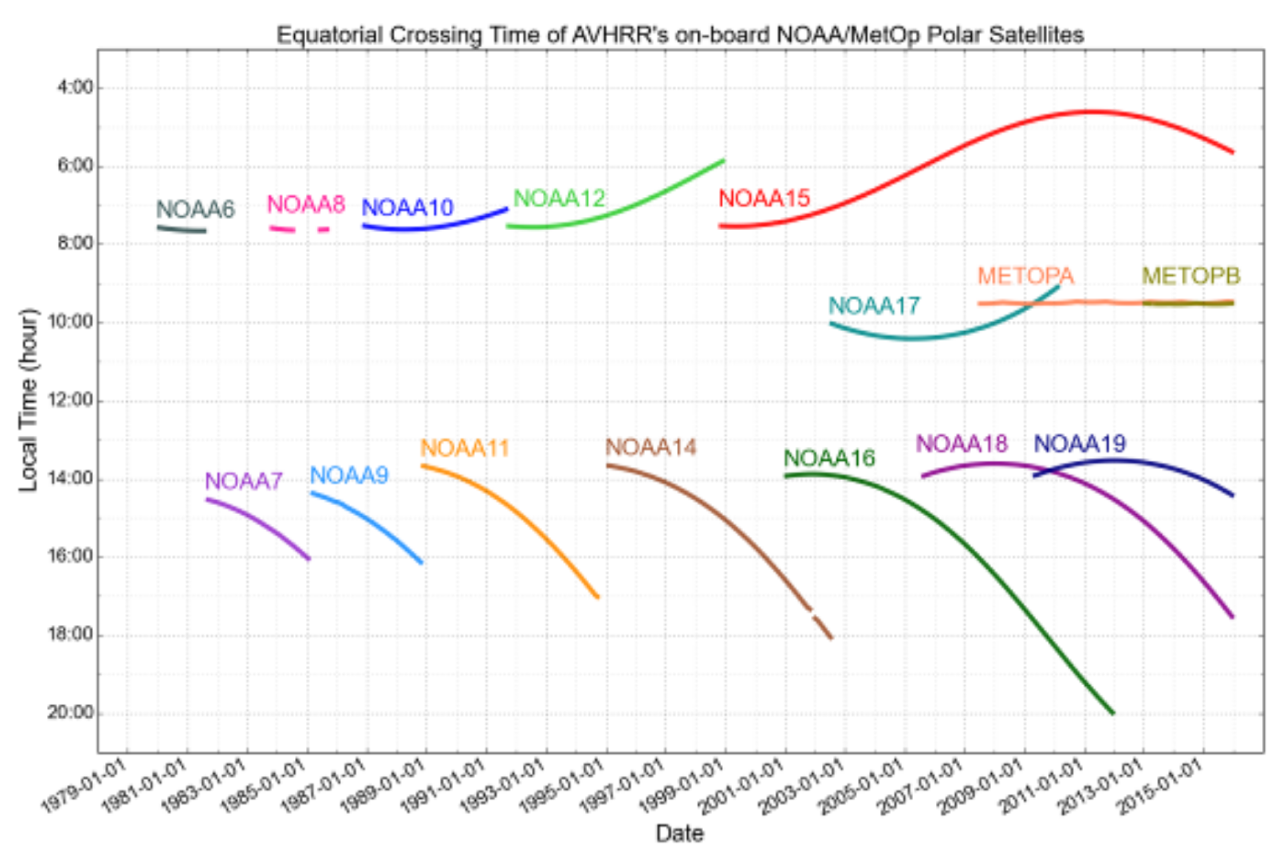
Figure 1. Equator Crossing Time (ECT) for the different NOAA and METOP satellites used in CLARA-A3. Figure taken from [6].
Remotesensing 12 00929 g001
Figure 2. Regional variation of the RMS error (Wm−2) in 1° × 1° latitude-longitude boxes. (a) is for the two channel regression (Equation (1)) and (b) when Channel 5 is not available (Equation (2)). The histograms are also given (right).
Remotesensing 12 00929 g002
Figure 3. Regional variation of the bias (Wm−2) in 1° × 1° latitude-longitude boxes. (a) is for the two channel regression (Equation (1)) and (b) when Channel 5 is not available (Equation (2)). The histograms are also given (right).
Remotesensing 12 00929 g003
Figure 4. Variation of the RMS error as a function of the Viewing Zenith Angle (VZA) for the two-channel regression with Equation (1) (black) and the regression without Channel 5 (red curve).
Remotesensing 12 00929 g004
Figure 5. Illustrative example of an OLR diurnal cycle in a single grid box (land cover: desert), modeled using a single satellite NOAA-19 (a) and using all available satellites (b). Note that the actual daily mean is based on the “UTC day”, as indicated on the top and bottom of the graph (0–24 h).
Remotesensing 12 00929 g005
Figure 6. Difference between the June 2012 monthly mean OLR calculated by using the individual satellites and the reference (calculated using all available satellites), with figure rows representing satellites METOP-A (a,b), NOAA-15 (c,d), NOAA-18 (e,f) and NOAA-19 (g,h). The columns distinguish linear temporal interpolation (left) and ERA5 diurnal cycle modeling over clear land pixels (right).
Remotesensing 12 00929 g006
Figure 7. Difference between the monthly mean OLR calculated by only using NOAA-19 and by only using NOAA-15, for April (a,b) and June (c,d) 2012, with (a,c) linear temporal interpolation and (b,d) ERA5 diurnal cycle modeling for clear land pixels.
Remotesensing 12 00929 g007
Figure 8. Monthly mean OLR difference with respect to CERES Synoptic 1° latitude 1° longitude gridded (SYN1deg) for April 2012 (left) and June 2012 (right) when all four satellites (METOP-A, NOAA-15, NOAA-17, NOAA-19) are processed.
Remotesensing 12 00929 g008
Figure 9. Monthly mean OLR difference with respect to CERES SYN1deg for April 2012 (left) and June (right) based on METOP-A and NOAA-19 (i.e., two satellites).
Remotesensing 12 00929 g009
Figure 10. Monthly mean OLR difference with respect to CERES SYN1deg for April 2012 (left) and June 2012 (right) based on a single satellite, with figure rows representing satellites METOP-A (a,b), NOAA-15 (c,d), NOAA-18 (e,f) and NOAA-19 (g,h).
Remotesensing 12 00929 g010
Figure 11. Monthly mean OLR difference with respect to CERES SYN1deg April 2012 (left) June 2012 (right) when both Channels 4 and 5 are used (top) and using only Channel 4 (bottom).
Remotesensing 12 00929 g011
Table 1. CM SAF CLARA edition summary.
ReleasePeriod CoveredVariables
CLARA-A1 [3]1982–2009Cloud products: fractional cloud cover, cloud top level,
cloud optical thickness, cloud effective radius, cloud phase,
liquid and ice water path, joint cloud histogram.
Radiation products: solar surface irradiance, surface albedo,
surface net short/longwave, surface downwelling/outgoing
longwave, surface radiation budget, cloud radiative effect.
CLARA-A2 [4]1982–2015idem as for CLARA-A1.
CLARA-A31979–2020idem as for CLARA-A1/A2, complemented by:
* (Surface) black sky and white sky albedo,
* (Top-of-atmosphere) Reflected Solar Flux (RSF),
* (Top-of-atmosphere) Outgoing Longwave Radiation (OLR).
Table 2. Statistics of the RMS error and bias of the OLR estimation with Equation (1) (2 channels) and Equation (2) (1 channel).
StatisticChannels5th PercentileMean95th Percentile
Wm−2Wm−2Wm−2
RMS error2 channels2.854.866.85
1 channel3.225.998.60
Bias2 channels−1.13−0.11+0.83
1 channel−1.41−0.06+1.27
Table 3. Mean OLR, bias, and RMS error of the OLR estimation with Equation (1) (2 channels) and Equation (2) (1 channel) for the NOAA-17, -18, and -19. The last column gives the multiplicative factors to be applied to the estimated OLR to remove the bias.
Mean OLR (AVHRR)Mean OLR (CERESBiasRMS ErrorFactor
Wm−2SSF) Wm−2Wm−2Wm−2
NOAA-17 with2ch216.14215.89+0.354.570.9982
CERES Terra1ch215.64−0.255.601.0011
NOAA-18 with2ch220.95220.98−0.034.881.0002
CERES Aqua1ch221.10+0.126.010.9996
NOAA-19 with2ch220.36221.13−0.774.781.0038
CERES Aqua1ch221.12−0.016.061.0001