Vertical Distribution of Arctic Methane in 2009–2018 Using Ground-Based Remote Sensing

Abstract

We analyzed the vertical distribution of atmospheric methane (CH${}_4$) retrieved from measurements by ground-based Fourier Transform Spectrometer (FTS) instrument in Sodankylä, Northern Finland. The retrieved dataset covers 2009–2018. We used a dimension reduction retrieval method to extract the profile information, since each measurement contains around three pieces of information about the profile shape between 0 and 40 km. We compared the retrieved profiles against Atmospheric Chemistry Experiment Fourier Transform Spectrometer (ACE-FTS) satellite measurements and AirCore balloon-borne profile measurements. Additional comparison at the lowest tropospheric layer was done against in-situ measurements from a 50-m-high mast. In general, the ground-based FTS and ACE-FTS profiles agreed within 10% below 20 km and within 30% in the stratosphere between 20 and 40 km. Our method was able to accurately capture reduced methane concentrations inside the polar vortex in the Arctic stratosphere. The method produced similar trend characteristics as the reference instruments even when a static prior profile was used. Finally, we analyzed the time series of the CH${}_4$ profile datasets and estimated the trend using the dynamic linear model (DLM).

1. Introduction

After carbon dioxide (CO${}_2$), methane (CH${}_4$) is the second most important anthropogenic greenhouse gas in the atmosphere. While methane is not as abundant, it traps about 28 times more heat per unit mass than carbon dioxide [1]. In comparison to carbon dioxide, methane is relatively short lived with a lifetime of around nine years [2]. Despite this, the concentration of atmospheric methane has more than doubled since pre-industrial times, with global average surface concentration being 1863 ppb in May 2019 [3,4].

Atmospheric methane is produced on the surface by both human activities and natural processes. Major sources of methane include agriculture, waste management, production and use of fossil fuels and different processes in the biosphere involving microorganisms and plants, especially in the wetlands [5]. Increased methane concentrations introduce a potential positive climate feedback in the Arctic in the form of emission changes from the wetlands and potential release of methane trapped in the permafrost caused by a warmer climate [6,7].

The main loss mechanism of methane, accounting for about 90% of the sink, is oxidation by the hydroxyl radical (OH), mainly in the troposphere [5]. In the troposphere, other notable sinks are oxidation in soils and loss by photochemistry in the marine boundary layer [5]. In the stratosphere, methane is lost in the reactions with OH, but also with atomic oxygen (O(${}^1$D)) and chlorine (Cl). The latter two account for 3% of the total methane sink, with O(${}^1$D) being more important closer to the equator and Cl at high latitudes [8].

While the main source of methane is on the surface, the sink is spread more evenly in the troposphere. This creates a negative vertical gradient in the tropospheric profile, especially close to a source where the emitted methane is not completely mixed vertically [9,10]. The stratospheric air in the Arctic originates from equatorial troposphere from where it slowly ascends to stratosphere and is transported towards the poles [11,12]. During the ascent and transport, methane is subject to chemical loss, which causes a negative vertical gradient in the stratosphere. During winter, the temperature of the polar stratosphere decreases because of reduced solar radiation. This creates a pressure gradient between high latitudes with the polar night and mid-latitudes. This pressure gradient together with the Earth’s rotation produces a circumpolar belt of westerly winds in the stratosphere called polar vortex [13]. Horizontal transport through the edge of the polar vortex is restricted and the air inside the vortex is descending. This results in an even larger gradient inside the vortex as the descending air has resided longer in the stratosphere, leading to a stronger depletion of methane [14].

The global growth rate of methane has varied in the recent decades. In the beginning of the 2000s, methane concentrations leveled off to what was suggested to be a possible steady state [15]. In 2007, however, methane concentration started to increase again [16]. The reasons for the stagnation and the renewed growth have been widely speculated but, thus far, a consensus has not been reached [5]. Saunois et al. [5] concluded that the most probable reasons for the latest rising trend are increased microbial and fossil emissions, with the tropics being the most probable region with the highest increase in emissions and the Arctic having a negligible effect. Changes in the OH sink can provide a partial explanation: Rigby et al. [17] showed that the OH sink was likely stronger during the stagnation period, which could explain the stable concentrations with a smaller decrease in emissions.

The concentrations of methane in the Arctic have been observed to follow the global behavior, increasing about 6 ppb/year (2008–2013) [7]. Since the recent increase in methane concentrations after 2007, the growth rate in the Arctic has been found to have a tendency to lag behind the rest of the world [18], suggesting that the increase is not of local or regional Arctic origin. During winter, methane levels in the Arctic are impacted by transport from mid-latitude source regions. During summer, local sources consist mostly of wetlands, confirmed by the isotopic data from Arctic measurement sites [7]. While Arctic methane emissions are expected to increase due to rising average temperatures, to date, no definitive changes in the Arctic methane emissions have been detected by the existing observational network [7].

Atmospheric methane can be measured with a variety of different techniques. Close to the ground level, a gas analyzer can be set up to sample surrounding air and analyze the methane concentration. Alternatively, an air sample can be collected to a flask and analyzed in a laboratory [19,20]. Using remote sensing, the total column of methane (XCH${}_4$) can be retrieved measuring the absorption of direct solar radiation at near-infrared or mid-infrared wavelengths. This method is used by the Total Carbon Column Observing Network (TCCON [21]) and the Network for the Detection of Atmospheric Composition Change (NDACC [22]). The infrared radiation back-scattered by the atmosphere and the surface is used by satellite instruments, such as TROPOMI onboard Sentinel 5 Precursor satellite (S5P [23]) and TANSO-FTS onboard GOSAT [24], to retrieve XCH${}_4$ from space.

While surface concentrations and total columns are measured continuously at numerous stations, the atmospheric profile of methane is usually measured in campaigns or rather infrequently by flying an instrument on an aircraft or using an AirCore [25]. An AirCore is a long, narrow stainless steel tube, which is lifted with an atmospheric sounding balloon up to about 30 km altitude. The tube then ingests the surrounding air while descending through the atmosphere. AirCore measurements are crucial for vertical distribution research; most aircraft are unable to reach altitudes above roughly 13 km [26] and therefore cannot measure the stratospheric profile that is highly variable for methane, especially at high latitudes inside the polar vortex [14].

Another way to measure atmospheric profiles is using a satellite with limb viewing geometry, which allows the satellite to scan through different layers of the atmosphere as the sun (or other star) is ascending from behind the horizon or descending behind it. This method is used by the FTS instrument onboard the Atmospheric Chemistry Experiment (ACE) satellite to retrieve atmospheric profiles of CH${}_4$ in the upper atmospheric layers. In this work, the ACE-FTS profile retrievals are used to evaluate our ground-based profile retrievals. A large ensemble of co-located ACE-FTS profiles is also used in the construction of the extra-tropospheric part of prior profiles.

In this work, we retrieved a time series of methane profiles from high-resolution short-wave infrared spectra measured by a ground-based Fourier Transform Spectrometer (FTS). Retrieval was done by modeling the temperature and pressure broadened absorption lines in short-wave infrared (SWIR) wavelength range using the Swirlab code that is publicly available [27]. Other remote sensing profile retrieval codes for ground-based FTS spectra were described and demonstrated by Hase et al. [28] and Zhou et al. [29]. The inverse problem related to the profile retrieval is ill-posed, thus, to retrieve physically meaningful profiles and to prevent artificial oscillations in the retrieved methane profile, the retrieval needs to be constrained. The other codes, PROFFIT [28] and SFIT4TCCON [29], use Tikhonov regularization [30] to obtain an appropriate prior for the retrieval. Swirlab on the other hand utilizes prior based dimension reduction [31], where the retrieved profile is constructed using only the largest singular vectors calculated from the prior covariance matrix. The prior itself is first built to reflect the mean and variability of the ACE-FTS measurements. An advantage of this method is that, in addition to regularization, the dimension of the problem is reduced, leading to a more computationally efficient retrieval algorithm [32].

The most significant advantage of the FTS measurements over the other profile measurements is the time resolution. The aircraft and balloon-borne measurements are superior in accuracy and vertical resolution. However, they are time consuming and resource intensive, and therefore not made on a daily or even weekly basis. Solar occultation measurements by ACE-FTS also have a higher vertical resolution than the ground-based remote sensing methods but the profiles cover only altitudes from roughly 10 km upwards. Due to the satellite’s orbit and measurement geometry, the revisit time over Sodankylä varies between 1 and 70 days. Temporary data gaps in the ground-based FTS measurements are caused by clouds blocking the direct view of the sun. Excluding the polar night, data gaps longer than two days are very rare.

While the profile information is useful in itself, the profile retrieval method could also improve the total column measurements. The averaging kernels show better sensitivity to the variability in the stratosphere than in the case of a profile scaling method [32]. In addition, the solar zenith angle (SZA) dependence of the averaging kernels is lower, thus resulting in reduced SZA-induced biases when the true profile differs significantly from the prior profile used for the retrieval [32].

To evaluate the performance of Swirlab retrievals, the profiles were here compared to concurrent ACE-FTS profiles above 10 km altitude, AirCore balloon measurements below 30 km and to 50-m mast measurements for the lowest atmospheric level of the profile. In addition to one-to-one comparisons, a dynamic linear model (DLM) trend analysis [33] was carried out to each dataset, and the growth rates of the recent years were compared. The growth rates were also evaluated in the light of recently published Arctic methane growth rates [7,10,18].

2. Data Description

The study concentrated on data measured at or above Finnish Meteorological Institute’s Arctic Space Centre in Sodankylä. The site is located at 67.37${}^{°}$N, 26.63${}^{°}$E (see Figure 1) and hosts a high-quality measurement infrastructure covering several research areas such as upper-air chemistry and physics, atmospheric column measurements, cryospheric and hydrological processes, biosphere—atmosphere interaction and satellite calibration and validation.

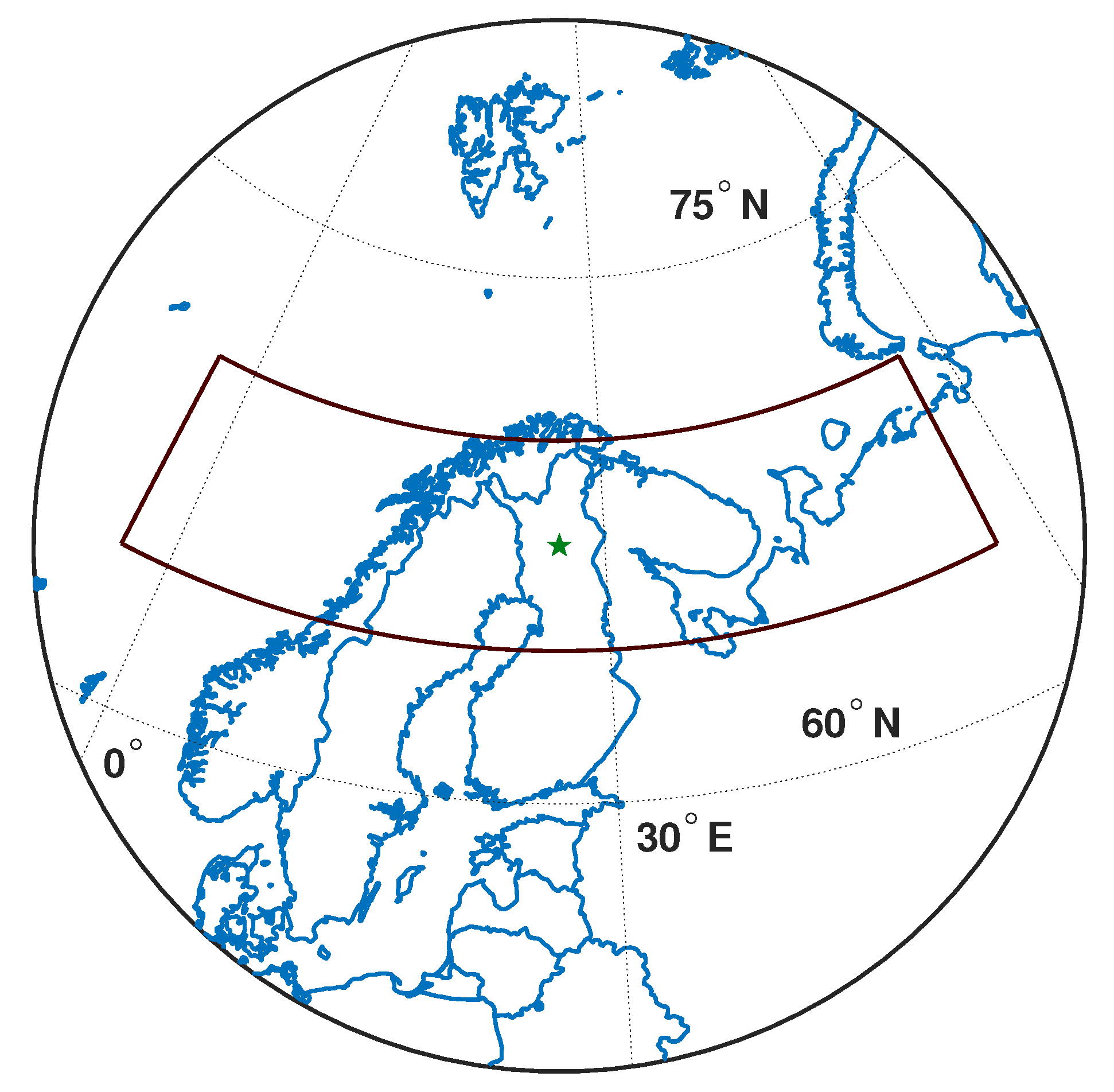
2.1. Ground-Based FTS Dataset

The Fourier Transform Spectrometer at Sodankylä became operational in 2009 [34]. The instrument participates in the Total Carbon Column Observing Network (TCCON). The TCCON facility at Sodankylä is equipped with a Bruker IFS 125HR spectrometer and a large solar tracker A547N (Bruker Optics, Ettlingen, Germany). The instrumentation is designed to record high-resolution solar spectra in the near-infrared spectral region. From the spectra, column-averaged abundances of CO${}_2$, CH${}_4$, N${}_2$O, HF, CO, H${}_2$O, HDO and other gases are derived.

The FTS instrument at Sodankylä has two room temperature detectors: an indium gallium arsenide (InGaAs, wavenumber range is 4000–11,000 cm${}^{-1}$) and a silicon diode (Si, range is 9000–15,000 cm${}^{-1}$). In addition, a liquid nitrogen cooled indium antimonide detector (InSb, detector covers 1800–6000 cm${}^{-1}$) was installed in July 2013. The additional detector expands the wavelength region covered by the instrument and provides a possibility to retrieve more atmospheric species. For stability and to keep water vapor low, the measurements are performed in vacuum. For the TCCON measurements, the spectral resolution is 0.02 cm${}^{-1}$, with an optical path difference of 45 cm and the collection time for a single scan is 78 s. The instrument has been operated in an automated mode: after two InGaAs/Si scans, one InSb scan is taken. The instrument characterization has been performed using a hydrogen chloride gas cell.

For the TCCON retrieval, GGG2014 algorithm is used [35]. The algorithm retrieves total column dry air mole fraction of methane using three wavelength windows centered at 5938, 6002 and 6076 cm${}^{-1}$ (1684, 1666 and 1647 nm). The spectroscopy is based on a modified HITRAN2012 line list [36]. The National Centers for Environmental Protection and National Center for Atmospheric Research (NCEP/NCAR) reanalysis data are used to generate prior profiles of pressure, temperature, geopotential height and water vapor. Methane prior profiles are generated by empirical functions that include a secular increase, interhemispheric gradient, seasonal cycle and stratospheric decay based on the age of air. These functions are optimized to fit existing information from balloon-borne platforms, satellites and aircraft campaigns. The prior CH${}_4$ profiles are iteratively scaled to generate forward-modeled spectra that best fit the measured spectra. To calculate the total column dry air mole fractions (XCH${}_4$), the total dry air columns are calculated from retrieved O${}_2$ columns, with a fair assumption of constant O${}_2$ dry air mole fraction (20.95%). An empirical correction is applied to correct the solar zenith angle (SZA) dependence, determining any variations that are symmetric about local noon as SZA-dependent artefacts [21]. The TCCON data are publicly available at the TCCON data archive, hosted by Caltech-DATA [37]. The algorithm to retrieve profile information from the same spectra is described in Section 3.1.

2.2. AirCore Measurements

The AirCore was constructed as a 100-m-long coated stainless steel tube, with a volume of about 1400 mL. A data logger was built to record the temperature of the AirCore and the ambient pressure. An automatic valve was used to close the inlet valve of the AirCore system shortly after the landing of the payload. The AirCore was lifted by a meteorological balloon to the altitude of typically 25–30 km, and was filled during descent from the stratosphere down to the surface. The gas analysis was performed typically within 2–3 h after the landing of the AirCore using a cavity ring-down spectrometer (CRDS). Calibration of the CRDS was performed before and after analyzing the sample to ensure the traceability of the measurements to the World Meteorological Organization scale of CH${}_4$ (X2004A).

2.3. ACE Data

Atmospheric Chemistry Experiment (ACE), also known as SCISAT, is a Canadian-led satellite mission for remote sensing of the Earth’s atmosphere. It was launched in August 2003. The primary instrument onboard is the infrared Fourier transform spectrometer (ACE-FTS). It measures infrared spectrum in the wavenumber range of 750–4400 cm${}^{-1}$ with a resolution of 0.02 cm${}^{-1}$. The spectra are measured during sunsets and sunrises in the limb viewing geometry with different slant paths and tangent heights from upper troposphere up to 150 km [38]. From the measured spectra, several tens of microwindows are analyzed to retrieve CH${}_4$ profiles with the vertical resolution of about 4 km. In the comparison studies, the accuracy has been found to be within 10% in the upper troposphere–lower stratosphere region [39].

To gather a comprehensive dataset, the co-location criteria for ACE-FTS measurements was set quite loose. Measurements within 30 degrees in longitude and 3 degrees in latitude from Sodankylä were included in the analysis (see map in Figure 1). The comparison between ACE-FTS and Swirlab was done on the spatially closest ACE-FTS profile of the day and the daily average of SZA-corrected Swirlab profiles. We used the Level 2 ACE-FTS data version 3.5 and 3.6 interpolated to a 1 km grid with center altitudes from 0.5 to 149.5 km. The analysis was restricted to altitudes from 10 to 40 km as the ACE-FTS data below 10 km are sparse and the sensitivity of the Swirlab retrieval is very low above 40 km.

2.4. Continuous Mast Measurements

Sodankylä 50-m-high mast has gas line inlets at four different heights: 2, 10, 23 and 50 m a.g.l. Sample air from highest level inlet is measured for 50 min/h, and air from two other (2 and 23 m) levels for 5 min/h each. The 10 m level is not measured regularly. Gas lines are 8-mm OD stainless steel, and they are flushed with flow rate of ca. 2.5 L/min, which corresponds to less than 1-min residence time in the lines.

Sample air is measured with a CRDS instrument, which measures CO${}_2$, CH${}_4$, CO and water vapor concentrations at the same time. This instrument is automatically calibrated with WMO/GAW/CCL (World Meteorological Organization/Global Atmosphere Watch/Central Calibration Laboratory, i.e., NOAA ESRL GMD) traceable calibration gases ca. 2 times a month. In addition, two cylinders, “working standard” and “target”, are measured every 11 and 34 h, respectively. The methane scale in use is WMO X2004A.

Humid air samples are measured directly, i.e., no dryer is used. This is compensated by determining and using individual water vapor correction factors for the instrument [40,41]. The raw data are first calculated as 1-min averages, and further to uncalibrated dry concentrations based on water vapor correction factors. Calibration is applied to these values, and hourly average concentrations are calculated from 1-min calibrated dry concentrations. For the time series analysis, a daily average value is calculated from the hourly values.

3. Methods

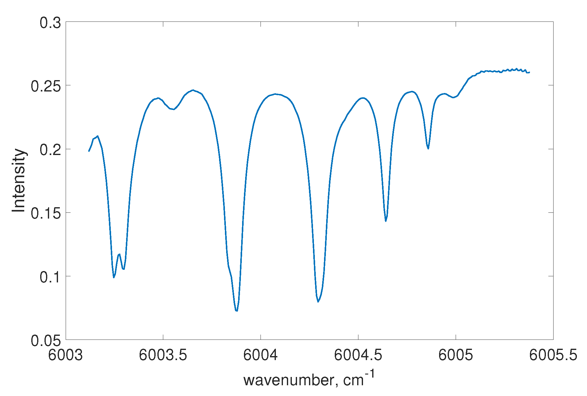
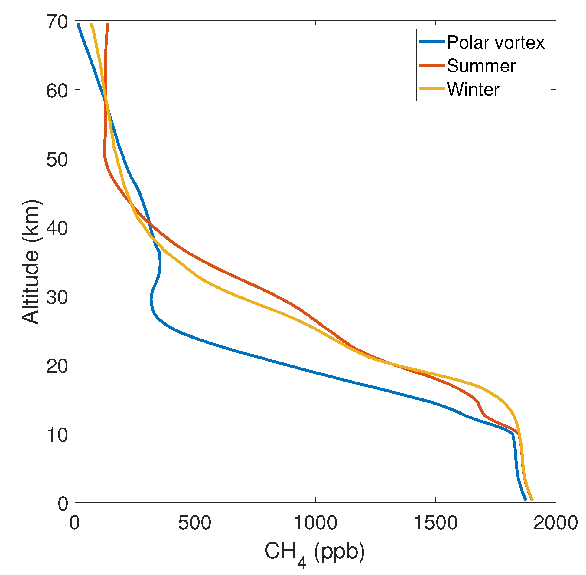
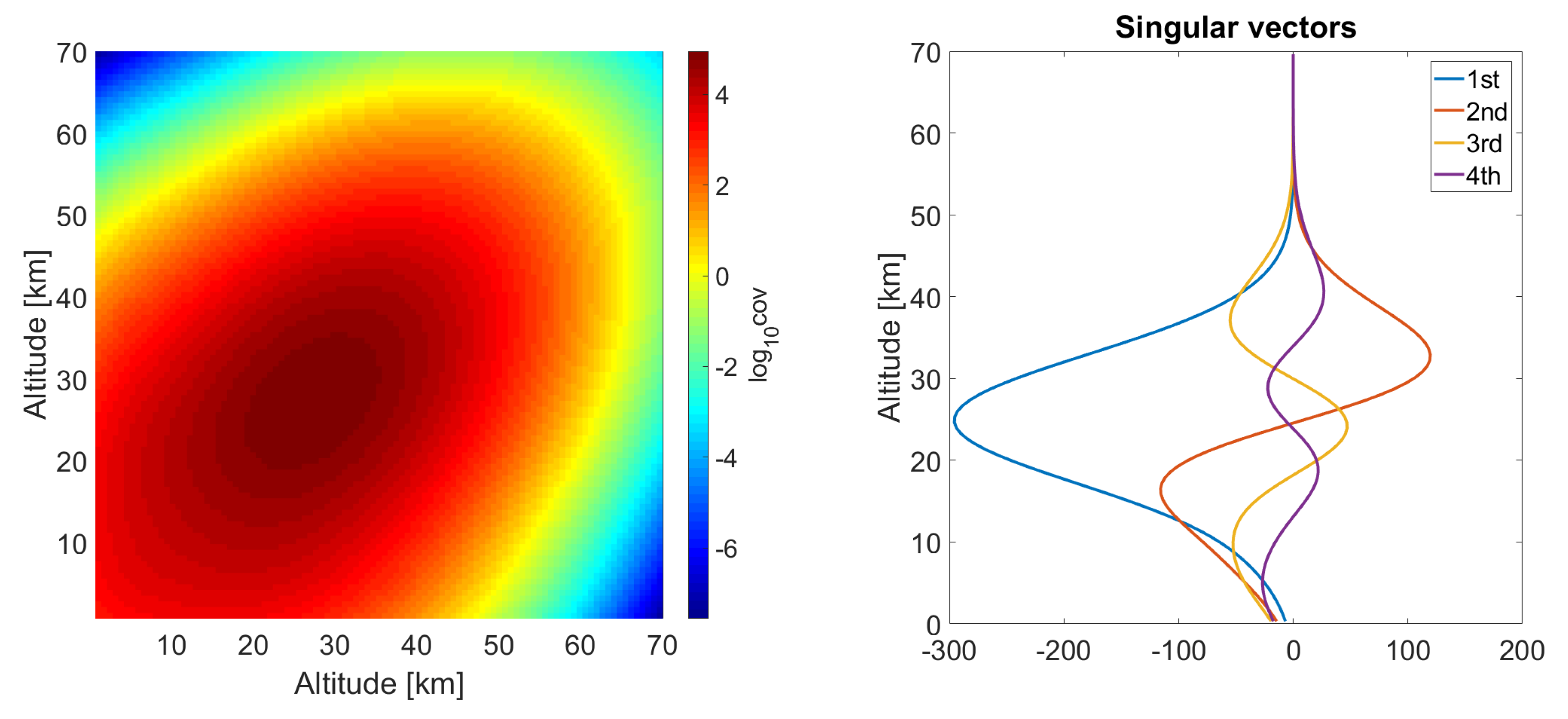
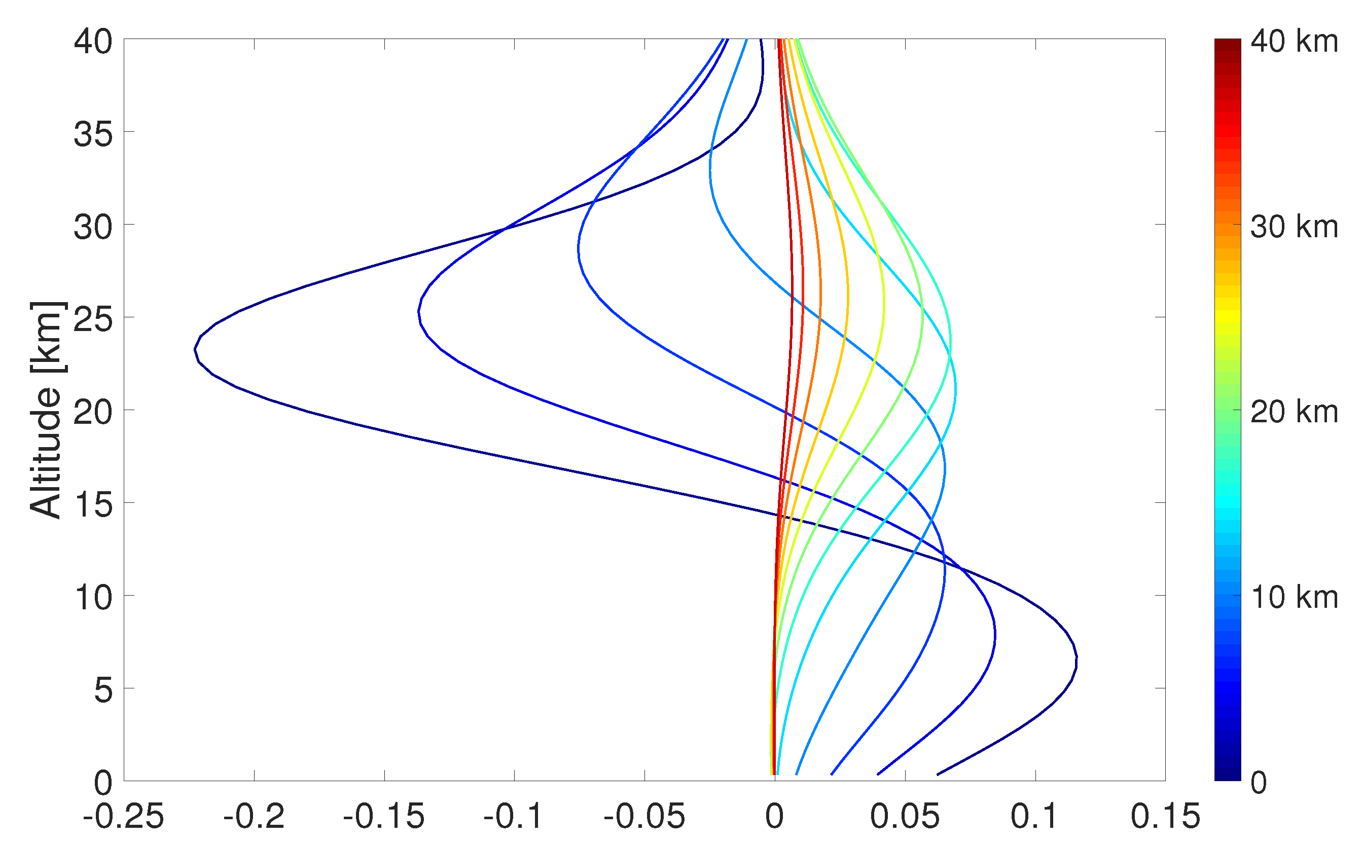
3.1. Profile Retrieval Method

Traditionally, ground-based direct solar radiation measurements at SWIR wavelengths have been used to retrieve methane total column. This is done by scaling the prior profile to produce a modeled spectrum that has the closest match to the measured spectrum (e.g., the method used in the TCCON retrievals [21]). However, the shapes of absorption lines include information about the vertical structure of the methane profile. The lines are broadened by temperature and pressure, resulting in wider absorption features at low altitudes and narrower at high altitudes. The algorithm described in this section finds the best fit between the modeled and measured spectra by allowing the methane profile shape to vary. This allows better fit between the measured and modeled spectra as also the width, in addition to the depth, of the absorption features in the modeled spectra is modified. The retrieved profiles, the vertically resolved concentrations and their changes can be studied. There are also advantages in using this method for total column retrievals: the averaging kernels show better sensitivity to the variability in the stratosphere than in the case of profile scaling method [32]. In addition, the SZA dependence of the averaging kernels is lower, thus resulting smaller SZA induced biases when there is a large difference between the shapes of the true profile and the prior profile used for the retrieval [32].

To retrieve vertical profiles of methane, we used the dimension reduction method described in detail in [32]. In this section, we give a brief description of the method. The goal has been to develop a method that would be only weakly dependent on the prior assumptions but would still provide information about the vertical structure and realistic profiles. The entire algorithm, hereafter referred to as Swirlab, is programmed to be run in Matlab and is publicly available [27].

The measured FTS data, described in Section 2.1, allows us to retrieve around 2–3 independent pieces of information about the vertical structure of CH${}_4$, as demonstrated in [32]. This means that we can actually extract more information from the measurement than the operational TCCON retrieval, which only has one degree of freedom. Thus, we construct the inverse problem so that there are 2–3 estimated parameters only. This kind of parameterization simplifies and stabilizes the inverse problem, and eases the computation in comparison to a layer-by-layer retrieval. The parameters need to be chosen so that they manifest the information content of the measurement, and we need a way to project the low-parameter profile back to the full space.

The profile of the atmospheric constituent of interest, in our cases CH${}_4$, is defined by first discretizing the atmosphere from 0 to 70 km into n layers and identifying the relative contribution of methane to the total atmospheric density (in parts per billion, ppb) per layer as $\overrightarrow{x}\in {\mathbb{R}}^n$. The inverse problem of inferring methane concentrations from measured data $\overrightarrow{y}\in {\mathbb{R}}^m$, also known as a retrieval, is derived from the relation

$$\overrightarrow{y}=f\left(\overrightarrow{x}\right)+\overrightarrow{\epsilon },$$

(1)

where f is a non-linear atmospheric radiative transfer model and $\overrightarrow{\epsilon }\in {\mathbb{R}}^m$ is a noise term describing the measurement and modeling error. The measured spectra used in this work are the same used for the TCCON retrieval but from a small microwindow with a wavenumber range from 6003 to 6005.5 cm${}^{-1}$ including five methane absorption lines. An example spectrum is given in Figure 2.

We use the Bayesian analysis for solving the retrieval problem and assume Gaussian distributions for the prior and noise, ${\overrightarrow{x}}_{pr}\sim \mathcal{N}({\overrightarrow{x}}_0,\mathbf{C}),\overrightarrow{\epsilon }\sim \mathcal{N}(0,{\mathbf{C}}_y)$, where ${\overrightarrow{x}}_0\in {\mathbb{R}}^n$ is a priori mean profile, $\mathbf{C}\in {\mathbb{R}}^{n\times n}$ positive definite prior covariance matrix and ${\mathbf{C}}_y\in {\mathbb{R}}^{m\times m}$ is the measurement error covariance matrix. The solution is obtained as posterior density of form

$$\overrightarrow{p}\left(\overrightarrow{x}\right|\overrightarrow{y})\propto exp\left(-\frac{1}{2}\left({\parallel \overrightarrow{y}-f\left(\overrightarrow{x}\right)\parallel }_{{\mathbf{C}}_y}^2+{\parallel \overrightarrow{x}-{\overrightarrow{x}}_0\parallel }_{\mathbf{C}}^2\right)\right).$$

(2)

We obtain the retrieved methane profile $\widehat{\overrightarrow{x}}$ from the retrieval method $\mathbf{R}$ as

$$\widehat{\overrightarrow{x}}=\mathbf{R}(\overrightarrow{y},{\mathbf{C}}_y,\overrightarrow{\theta }),$$

(3)

where $\mathbf{R}$ includes our prior assumptions, forward model and Bayesian formulation as well as additional parameters $\overrightarrow{\theta }$ such as pressure, solar parameters, etc. These parameters can be retrieved as a part of the state vector, but to keep the notation compact we keep them fixed.

The model atmosphere consists of a non-scattering atmosphere with 100 spherical layers from ground level up to 70 km. Absorption lines are calculated for each layer separately as Voigt profiles taking into account the temperature and pressure of the layer. Atmospheric model data from National Centers for Environmental Prediction (NCEP) are used as source for these atmospheric parameters. As an update to description in Tukiainen et al. [32], the absorption coefficients are calculated using HITRAN2016 line database [42].

The dimension reduction approach that we adapted is based on those of Marzouk and Najm [43] and Solonen et al. [31]. The fundamental idea is to constrain the problem to a subspace that contains most of the variability allowed by the prior. This is achieved by using a smoothing prior covariance that has only a small amount of singular values significantly greater than zero, and thus most of this variability can be represented by a linear combination of the corresponding leading singular vectors. Thus, we start with the singular value decomposition of the prior covariance matrix

$$\mathbf{C}=\mathbf{U}\mathsf{\Lambda }{\mathbf{U}}^T,$$

(4)

where the diagonal matrix $\mathsf{\Lambda }$ contains the singular values of the prior covariance matrix and $\mathbf{U}$ contains the corresponding singular vectors ${\overrightarrow{u}}_1,\dots ,{\overrightarrow{u}}_n$ as columns. The dimension of the problem is then reduced by using the k ($1\le k<n$) largest singular values and the corresponding singular vectors and representing the unknown as a linear combination

$$\overrightarrow{x}={\overrightarrow{x}}_0+{\mathbf{P}}_k{\overrightarrow{z}}_k,{\mathbf{P}}_k={\mathbf{U}}_k{\mathsf{\Lambda }}_k^{\frac{1}{2}}=\left[\sqrt{{\lambda }_1}{\overrightarrow{u}}_1,\sqrt{{\lambda }_2}{\overrightarrow{u}}_2,\dots ,\sqrt{{\lambda }_k}{\overrightarrow{u}}_k\right].$$

(5)

Here, the new unknown ${\overrightarrow{z}}_k$ is a k-dimensional vector whose prior distribution is a k-dimensional Gaussian $\mathcal{N}(0,{\mathbf{I}}_k)$ and ${\mathbf{P}}_k\in {\mathbb{R}}^{n\times k},k<n$, is a projection matrix from ${\mathbb{R}}^k$ to ${\mathbb{R}}^n$. Inserting this new parameterization to the problem leads to a posterior distribution for the subspace parameter ${\overrightarrow{z}}_k$ of the form

$$\overrightarrow{p}\left(\overrightarrow{z}\right|\overrightarrow{y})\propto exp\left(-\frac{1}{2}\left({\parallel \overrightarrow{y}-f({\overrightarrow{x}}_0+{\mathbf{P}}_k{\overrightarrow{z}}_k)\parallel }_{{\mathbf{C}}_y}^2+{\parallel \overrightarrow{z}\parallel }_{{\overrightarrow{I}}_k}^2\right)\right).$$

(6)

The prior mean, ${\overrightarrow{x}}_0$, is estimated by combining the stratospheric part from the ACE-FTS satellite data and the tropospheric part from the TCCON prior data. The prior is calculated separately for three domains: summer (from May to August), polar vortex and the rest (denoted as winter). The location inside the polar vortex is defined using ERA-Interim atmospheric model data. The station is assumed to be inside the polar vortex when potential vorticity at 475 K potential temperature level exceeds 3$\times {10}^{-5}\mathrm{K}{\mathrm{m}}^2{\mathrm{s}}^{-1}\mathrm{kg}$. The seasonal prior means are depicted in Figure 3. A trend of 5.57 ppb per year, determined from the TCCON prior profiles 2009–2016, is added to each layer. In addition, retrieval with trendless prior is made and the effect is discussed in Section 4.2.

For the prior covariance construction, we follow the procedure from Tukiainen et al. [32] to produce a variability that matches well to the empirical covariance derived from an ensemble of ACE-FTS satellite based measurements. In short, this is done by first computing the diagonal elements of $\mathbf{C}$ as

$$\sigma \left(h\right)={\sigma }_{1}exp\left(-{(h-h_1)}^2{s}_1^{-2}\right)+{\sigma }_{2}exp\left(-{(h-h_2)}^2{s}_2^{-2}\right),$$

(7)

where h are the atmospheric layers and the parameters ${\sigma }_1,{\sigma }_2,h_1,h_1,s_1$ and $s_2$ are chosen appropriately (${\sigma }_1$ = 300, ${\sigma }_2$ = 30, $h_1$ = 25, $h_2$ = 5, $s_1$ = 10 and $s_2$ = 5). The off-diagonal terms are further given by

$$c_{ij}=\sigma \left(i\right)\sigma \left(j\right)exp\left(-\frac{1}{2}{\left(\frac{\mathrm{dist}(i,j)}{l}\right)}^2\right),$$

(8)

where i and j are two atmospheric layers, $\mathrm{dist}(i,j)$ is the distance between these layers in kilometers and l is an appropriately chosen correlation length (l = 12 km). The full covariance matrix and the first four singular vectors are presented in Figure 4.

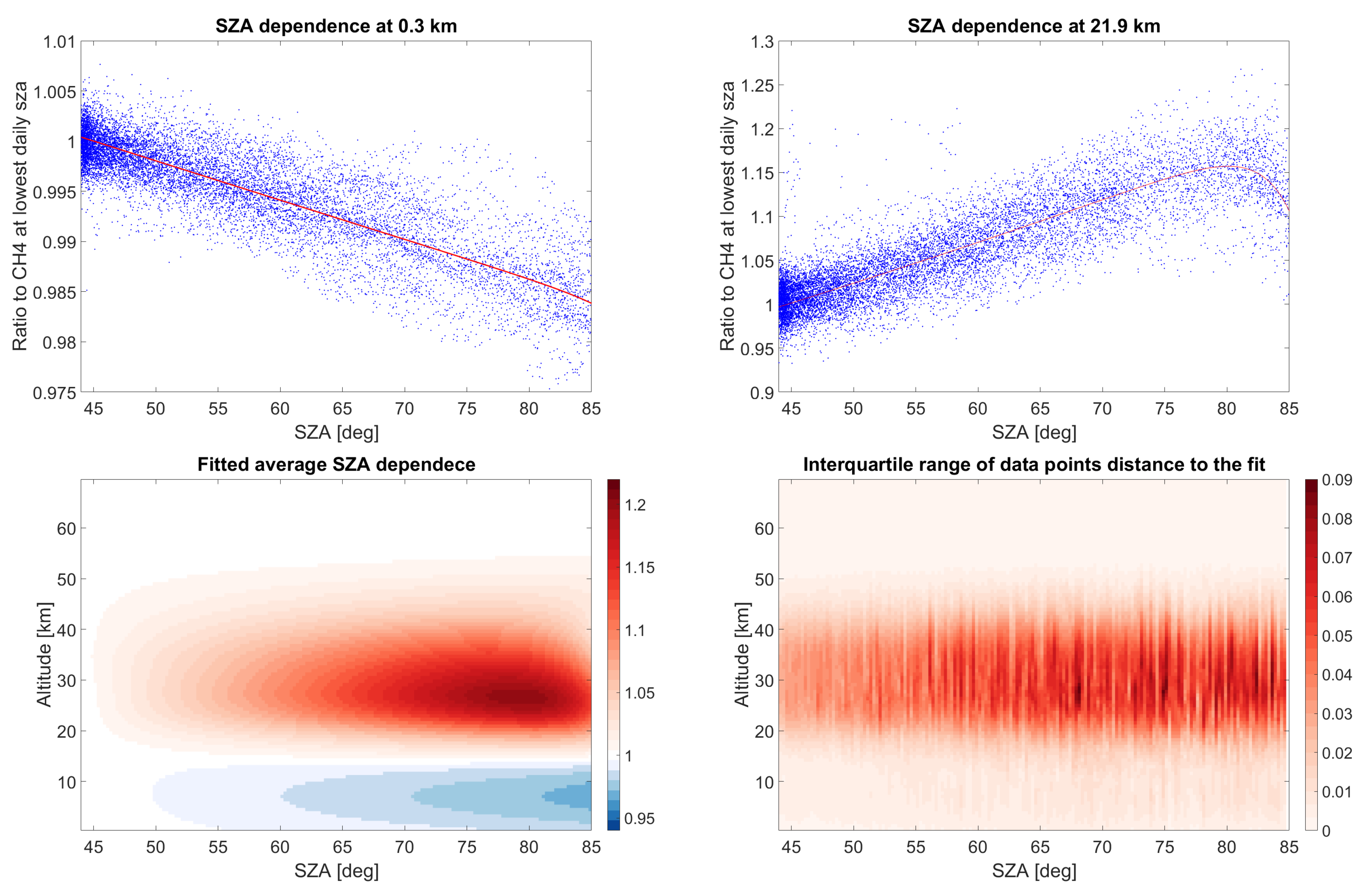
Solar Zenith Angle Dependence

Due to errors in radiative transfer modeling and spectroscopy, and because the measurements sensitivity to atmospheric composition at different altitudes changes when solar zenith angle (SZA) changes, there is a systematic difference between volume mixing ratios (VMR${}_{C{H}_4}$) measured at noon and at early morning or late evening (see Figure 5). This difference is compensated for by going through data for days when the SZA has had both small and large values. The measurement with the smallest SZA for the day is regarded as the reference value (REF${}_{C{H}_4}$) and the ratio (R) between all the daily measurements and the reference value is calculated.

$$\mathrm{R}=\frac{{\mathrm{VMR}}_{C{H}_4}}{{\mathrm{REF}}_{C{H}_4}}$$

(9)

The R is first calculated for days with the minimum SZA smaller than 44.5 degrees. Before calculating the ratios for the rest of the days, an exponential function

$$f_{corr}\left(\mathrm{SZA}\right)=aexp\left(b\mathrm{SZA}\right)+cexp\left(d\mathrm{SZA}\right)$$

(10)

is fitted to ratios R. For the days with the minimum SZA larger than 44.5 degrees, the reference value is corrected with this function and the following ratios are defined as

$$\mathrm{R}=\frac{{\mathrm{VMR}}_{C{H}_4}}{{\mathrm{REF}}_{C{H}_4}}{f}_{corr}\left({\mathrm{SZA}}_{\mathrm{ref}}\right),$$

(11)

where ${\mathrm{SZA}}_{\mathrm{ref}}$ is the smallest SZA of the evaluated day. The days are evaluated in order of minimum daily SZA. After each evaluated day, the $f_{corr}$ is updated and the evaluation ends when 10% of the time series (about 13,000 measurements) have been evaluated. Then, the final $f_{corr}$ is regarded as the zenith angle correction function for the time series. The correction function is calculated for each retrieved layer separately. The final corrected volume mixing ratio (cVMR${}_{C{H}_4}$) at layer i is then calculated as

$${\mathrm{cVMR}}_{C{H}_4,i}={\mathrm{VMR}}_{C{H}_4,i}{f}_{corr,i}\left(\mathrm{SZA}\right).$$

(12)

As an example, the SZA dependence of the volume mixing ratios at two different layers are depicted in Figure 5. The Figure also depicts the fits for all the layers and the spread of the difference between data points and the fit. The variability of the data points is described with interquartile range as there are some outliers skewing the distribution so that standard deviation would not describe the data well. Assuming that on average the methane concentration is stable and should not vary as a function of the solar zenith angle, it seems that at the layers close to the ground the mixing ratios are underestimated when the SZA increases, and in the stratosphere the values are overestimated when the sun is close to the horizon.

3.2. Averaging Kernel Correction to ACE Data

To compare the atmospheric profiles obtained from ACE-FTS measurements with Swirlab retrievals, the results must first be projected into the same space. This is because the ill-defined inverse problem is regulated by prior information and the retrieval is hence a biased estimator of true CH${}_4$. Moreover, the instruments naturally have different sensitivities at different altitudes, which needs to be accounted for as well. A widely used way to make two separate measurements by different instruments comparable is smoothing using the averaging kernel

$$\mathbf{A}=\frac{\partial \widehat{\overrightarrow{x}}}{\partial \overrightarrow{x}},$$

(13)

which measures the sensitivity of the retrieved value $\widehat{\overrightarrow{x}}$ to the actual true atmospheric state $\overrightarrow{x}$. Averaging kernels for $\overrightarrow{z}$ parameters can be estimated from the known Swirlab measurements using Jacobians, i.e., the derivatives of forward model f of the form ${\mathbf{K}}_{\mathbf{ij}}=\frac{{\partial }_i}{\partial x_j}f$, as

$${\mathbf{A}}_z=\frac{\partial \widehat{\overrightarrow{z}}}{\partial \overrightarrow{x}}={\left({\mathbf{K}}_k^T{\mathbf{C}}_y^{-1}{\mathbf{K}}_k+{\mathbf{I}}_k\right)}^{-1}\left({\mathbf{K}}_k^T{\mathbf{C}}_y^{-1}{\mathbf{K}}_v\right)$$

(14)

where ${\mathbf{A}}_z\in {\mathbb{R}}^{k\times n}$, ${\mathbf{C}}_y\in {\mathbb{R}}^{m\times m}$ is the error covariance matrix, ${\mathbf{I}}_k\in {\mathbb{R}}^{k\times k}$ is the prior covariance of ${\overrightarrow{z}}_k$,

$$\begin{array}{cc}\hfill & {\mathbf{K}}_k=\mathbf{K}\mathrm{diag}\left(\overrightarrow{l}({\mathbf{P}}_k{\overrightarrow{z}}_k+{\overrightarrow{x}}_0)\right){\mathbf{P}}_k\hfill \\ \hfill & {\mathbf{K}}_v=\mathbf{K}\mathrm{diag}\left(\overrightarrow{l}\right)\hfill \end{array}$$

(15)

and $\overrightarrow{l}\in {\mathbb{R}}^n$ contains the slant lengths of different atmospheric layers (for details, please refer to [32]). The full-state averaging kernel can then be computed as

$$\mathbf{A}=\mathrm{diag}({\mathbf{P}}_k{\overrightarrow{z}}_k+{\overrightarrow{x}}_0){\mathbf{P}}_k{\mathbf{A}}_z$$

(16)

where $\mathbf{A}\in {\mathbb{R}}^{n\times n}$. The averaging kernels are SZA dependent, and thus can partly contribute to diurnal and also seasonal biases. A Swirlab averaging kernel matrix at SZA = 45${}^{°}$ is visualized in Figure 6. We see that the changes in the lowest altitudes have a large effect to the higher levels also. As the covariance structure allows the profile to vary the most at altitudes between 20 and 30 km, many of the changes at levels that are more restricted to follow the prior propagate to these altitudes.

Using the Swirlab averaging kernel, we follow [44] and get the smoothed ACE-FTS profile as

$${\overrightarrow{x}}_{\mathrm{smooth}}={\overrightarrow{x}}_0+\mathbf{A}({\overrightarrow{x}}_{\mathrm{ACE}}-{\overrightarrow{x}}_0).$$

(17)

3.3. Time Series Analysis

In this study, our main interest is the altitude-dependent trend in the Sodankylä FTS time series. In general terms, trend can be defined as a change of distributional processes (e.g., mean) of the process that generates the observations. Typically, the interesting part is the more slowly varying background level after better-known variabilities, such as seasonality, have been accounted for. For time series trend analysis, we follow the approach by Laine et al. [45] and apply dynamical linear regression to the FTS data by using Dynamic Linear Model (DLM) toolbox for Matlab by Marko Laine [46]. In contrast to the more usual linear regression, dynamical regression allows the regression coefficient to evolve in time. This evolution is controlled by model variance parameters that are estimated from the data. DLM in extremely useful in atmospheric time series analysis since a lot of factors, such as external forcing, make the background mean trend nonlinear. On top of this, atmospheric processes are often a combination of short term rapid changes, such as seasonal cycles, and more long term background processes.

We present a short description of the DLM formulation used in our analysis. DLM with Gaussian errors is best described as a general linear state space model with an observation equation and an evolution equation as

$$\begin{array}{cc}\hfill & {\overrightarrow{y}}_t={\mathbf{H}}_t{\overrightarrow{u}}_t+{\overrightarrow{v}}_t,{\overrightarrow{v}}_t\sim \mathcal{N}(0,{\mathbf{R}}_t),\hfill \\ \hfill & {\overrightarrow{u}}_t={\mathbf{M}}_t{\overrightarrow{u}}_{t-1}+{\overrightarrow{w}}_t,{\overrightarrow{w}}_t\sim \mathcal{N}(0,{\mathbf{Q}}_t),\hfill \end{array}$$

(18)

where ${\overrightarrow{y}}_t$ contains the observations and ${\overrightarrow{u}}_t$ the hidden and unobserved model state at time step t, the observations are gained via the observation operator ${\mathbf{H}}_t$, the state is evolving along the model evolution operator ${\mathbf{M}}_t$. In this formulation, the observation error ${\overrightarrow{v}}_t$ and the model error ${\overrightarrow{w}}_t$ are assumed to be zero mean Gaussian with covariance matrices given by ${\mathbf{R}}_t$ and ${\mathbf{Q}}_t$, respectively.

The hidden state vector $\overrightarrow{u}$ has components for each process that is fitted in the time series analysis. In our case, we get

$${\overrightarrow{u}}_t=\left[{\mu }_t{\alpha }_t{\beta }_{t,1}{\beta }_{t,2}{\eta }_t\right],$$

(19)

where ${\mu }_t$ is the parameter for the local mean, ${\alpha }_t$ is for local trend, ${\beta }_{t,1}$ and ${\beta }_{t,2}$ represent the seasonal components and ${\eta }_t$ is the autoregressive component of the state vector.

In DLM, the background trend is modeled as a random walk process defined by local mean ${\mu }_t$ and local trend ${\alpha }_t$. For these parameters, we can write the observation operator, model evolution operator and model error as

$$\begin{array}{cccc}\hfill & {\mathbf{M}}_{\mathrm{trend}}\hfill & \hfill =& \left[\begin{array}{cc}1& 1\\ 0& 1\end{array}\right],\hfill \\ \hfill & {\mathbf{H}}_{\mathrm{trend}}\hfill & \hfill =& \left[\begin{array}{cc}1& 0\end{array}\right],\hfill \\ \hfill & {\mathbf{Q}}_{\mathrm{trend}}\hfill & \hfill =& \left[\begin{array}{cc}0& 0\\ 0& {\sigma }_{\mathrm{trend}}^2\end{array}\right],\hfill \end{array}$$

(20)

where ${\sigma }_{\mathrm{trend}}^2$ is the error variance of the local trend. Similarly, the annual seasonal cycles are modeled using harmonic functions. For seasonal components ${\beta }_{t,1}$ and ${\beta }_{t,2}$, we thus have

$$\begin{array}{cccc}\hfill & {\mathbf{M}}_{\mathrm{seas}}\hfill & \hfill =& \left[\begin{array}{cc}cos(2\pi /s)& sin(2\pi /s)\\ -sin(2\pi /s)& cos(2\pi /s)\end{array}\right],\hfill \\ \hfill & {\mathbf{H}}_{\mathrm{seas}}\hfill & \hfill =& \left[\begin{array}{cc}1& 0\end{array}\right],\hfill \\ \hfill & {\mathbf{Q}}_{\mathrm{seas}}\hfill & \hfill =& \left[\begin{array}{cc}{\sigma }_{\mathrm{seas}}^2& 0\\ 0& {\sigma }_{\mathrm{seas}}^2\end{array}\right],\hfill \end{array}$$

(21)

where $s=365.242$ is the number of days in a year (accounting also for leap years) and ${\sigma }_{\mathrm{seas}}^2$ is the error variance of the seasonal components. In this work, we also allow autocorrelations in the residuals by using a first-order autoregressive model. The corresponding observation operator, model evolution operator and model error are given by

$$\begin{array}{cccc}\hfill & {\mathbf{M}}_{\mathrm{AR}}\hfill & \hfill =& \left[\begin{array}{c}\rho \end{array}\right],\hfill \\ \hfill & {\mathbf{H}}_{\mathrm{AR}}\hfill & \hfill =& \left[\begin{array}{c}1\end{array}\right],\hfill \\ \hfill & {\mathbf{Q}}_{\mathrm{AR}}\hfill & \hfill =& \left[\begin{array}{c}{\sigma }_{\mathrm{AR}}^2\end{array}\right],\hfill \end{array}$$

(22)

Combining the independent parts for trend, seasonality and autoregression, we get the full observation operator, model evolution operator and model error for the hidden state vector $\overrightarrow{u}$ as

$$\begin{array}{cccc}\hfill & \mathbf{M}\hfill & \hfill =& \left[\begin{array}{ccc}{\mathbf{M}}_{\mathrm{trend}}& 0& 0\\ 0& {\mathbf{M}}_{\mathrm{seas}}& 0\\ 0& 0& {\mathbf{M}}_{\mathrm{AR}}\end{array}\right],\hfill \\ \hfill & \mathbf{H}\hfill & \hfill =& \left[\begin{array}{ccc}{\mathbf{H}}_{\mathrm{trend}}& {\mathbf{H}}_{\mathrm{seas}}& {\mathbf{H}}_{\mathrm{AR}}\end{array}\right],\hfill \\ \hfill & \mathbf{Q}\hfill & \hfill =& \left[\begin{array}{ccc}{\mathbf{Q}}_{\mathrm{trend}}& 0& 0\\ 0& {\mathbf{Q}}_{\mathrm{seas}}& 0\\ 0& 0& {\mathbf{Q}}_{\mathrm{AR}}\end{array}\right].\hfill \end{array}$$

(23)

With the previous formulation, the DLM algorithm proceeds with Kalman Filter and Simulation Smoother to generate an ensemble of states that fit the observed data. This step is repeated with Markov chain Monte Carlo (MCMC), sampling the parameters ${\sigma }_{\mathrm{trend}},{\sigma }_{\mathrm{seas}}$, ${\sigma }_{\mathrm{AR}}$ and $\rho$. This procedure explores various choices of tuning parameters for the problem and gives the values that fit the observations the best, minimizing arbitrary fixing that is often done manually in other applications. For a detailed description of the Simulation Smoother and the MCMC, we refer the reader to the documentation in [45,46].

4. Results

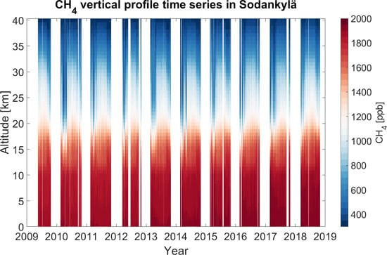
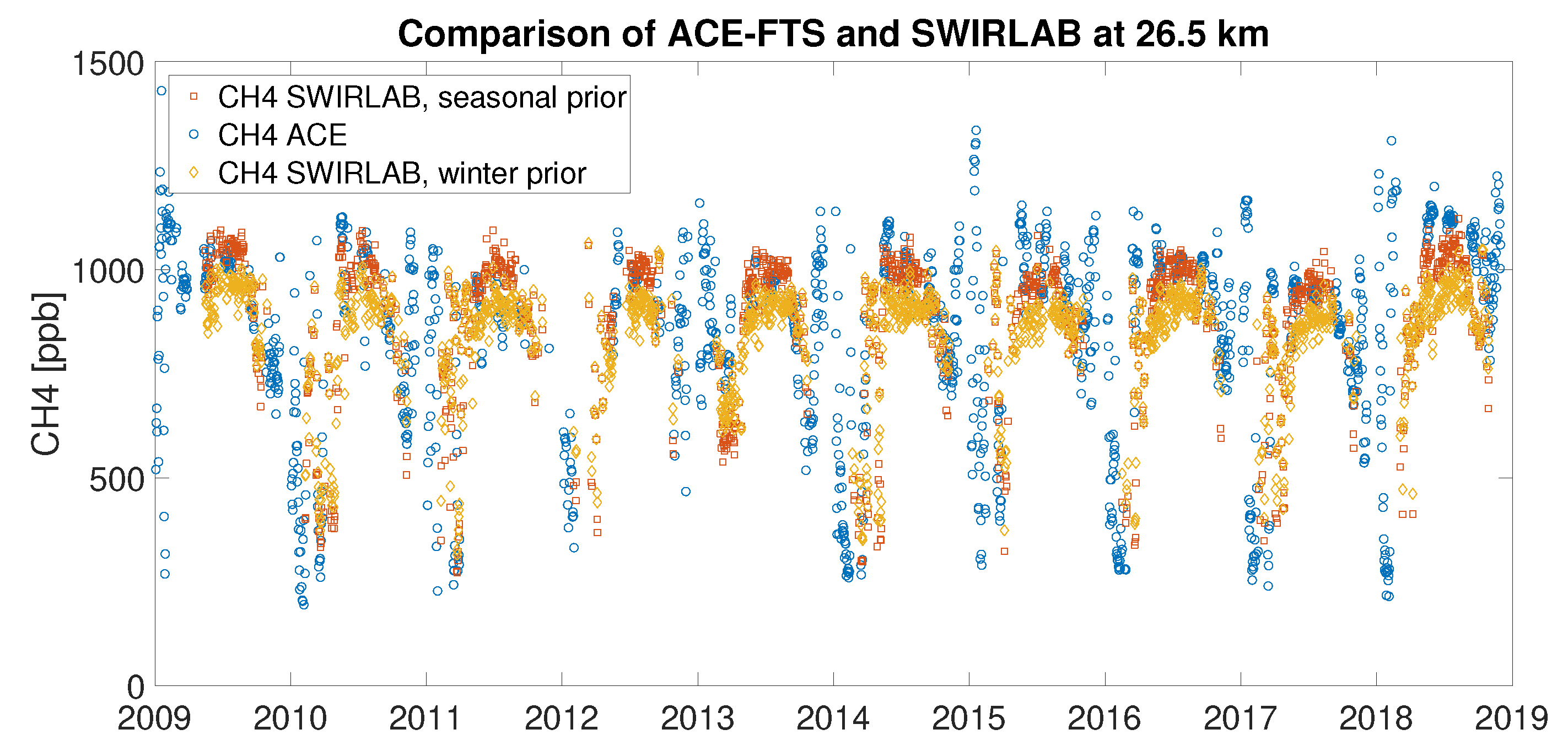
4.1. The Time Series

The Swirlab profile retrieval algorithm was used to retrieve methane profiles from all the SWIR spectra measured when non-obstructed sunlight was available in Sodankylä between May 2009 and November 2018. For further analysis and illustrative purposes, a time series of daily averages was calculated. Figure 7 shows a surface plot of the time series. In the figure, gaps shorter that seven days are filled and only few data gaps remain during the measurement season. The measurement season covers the time when the daily maximum solar elevation angle exceeds eight degrees, in Sodankylä roughly from mid-February to the end of October. On average there were 148 days with measurements per year between 2010 and 2018. The algorithm produces nicely the seasonal variability with summer minimum in the lower troposphere and really low values in the stratosphere throughout the spring when Sodankylä lies beneath the polar vortex. The seasonal behavior and trends at various altitudes are more closely studied in Section 4.6.

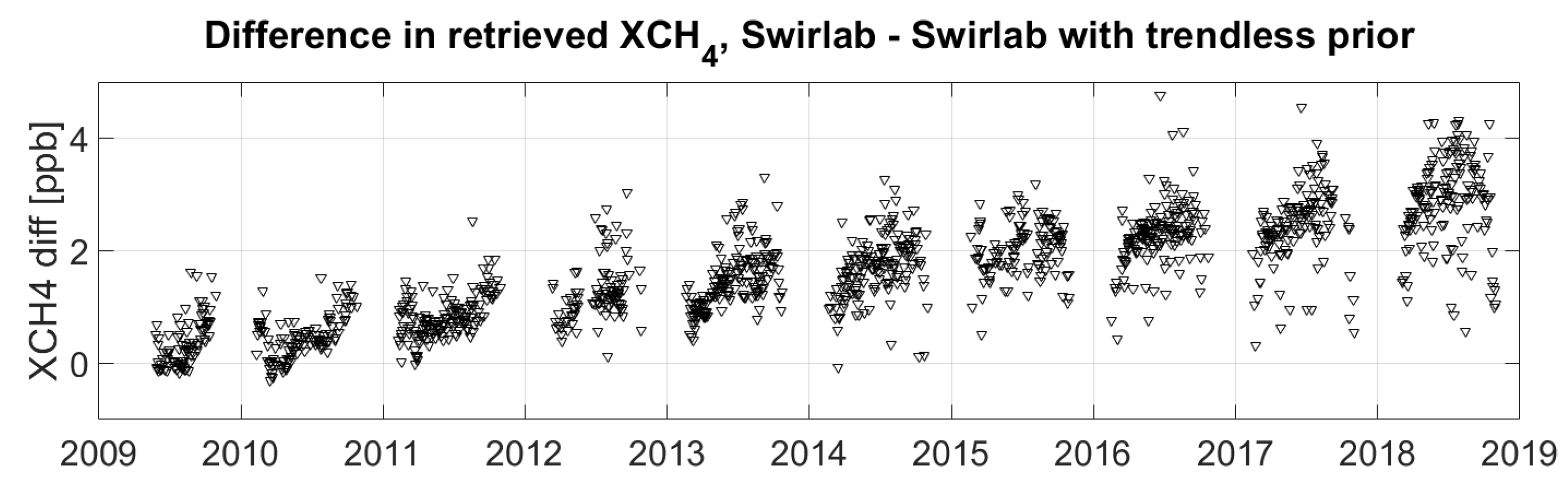
4.2. Sensitivity to Prior Profile

To demonstrate the profile information content in the ground-based FTS spectrum, we ran the Swirlab retrieval with different prior profiles. Even when using a single prior profile (Figure 8), the algorithm is able to detect the dip in stratospheric methane concentration inside the polar vortex. The use of a seasonal prior lets the retrievals inside the vortex reach a bit lower level. The introduction of the seasonal prior for summer also makes Swirlab retrieval agree better with the ACE-FTS mixing ratios (see (Figure 8) when the retrieval with a single prior leaves the summer values somewhat low compared to ACE-FTS.

Figure 9 shows the difference in total column mixing ratios calculated from Swirlab profiles with and without a trend in the prior. Swirlab is able to retrieve a positive trend in the methane total column even when the trend is excluded from the prior. However, the trend is roughly 0.3 ppb/year smaller than the one retrieved when a prior trend of 5.57 ppb/year is introduced. The prior trend is the average trend of total methane column calculated from TCCON prior profiles. The total column methane retrieved with prior trend agrees well with the TCCON data (see Section 4.5).

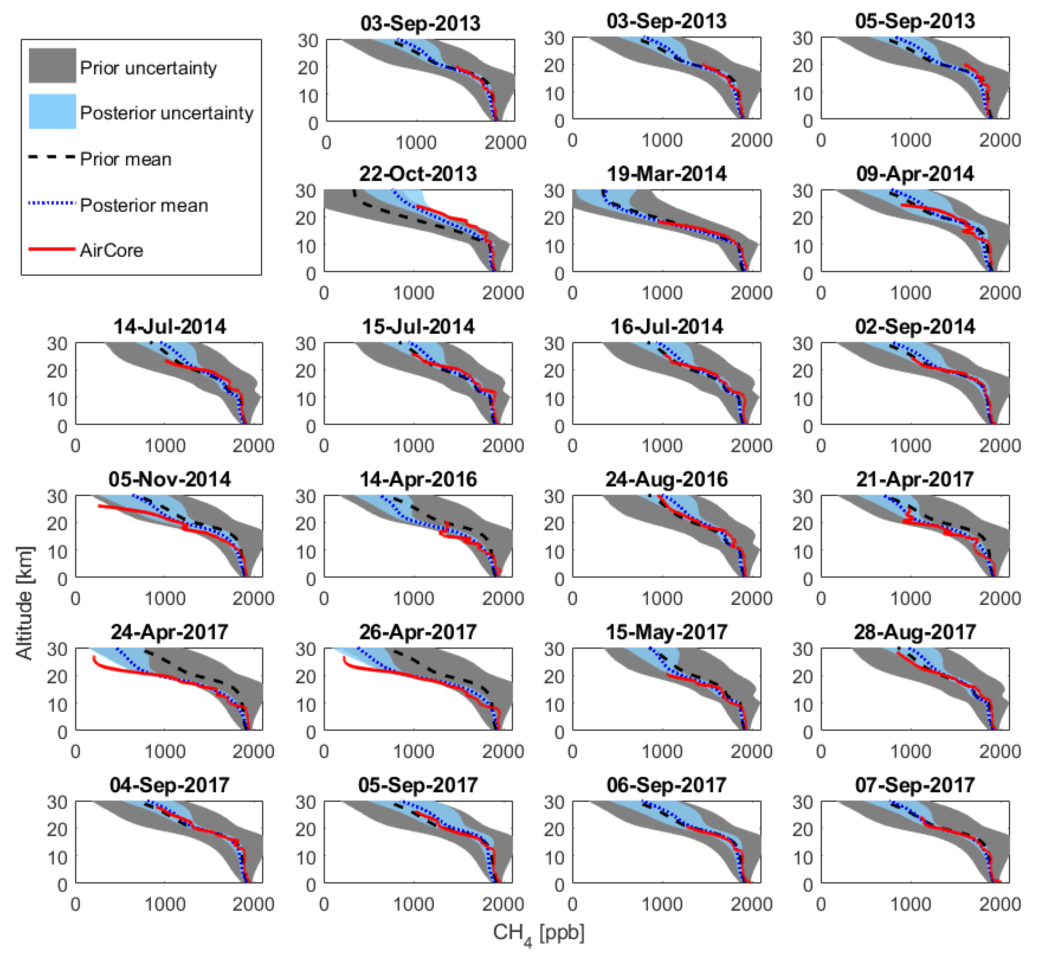
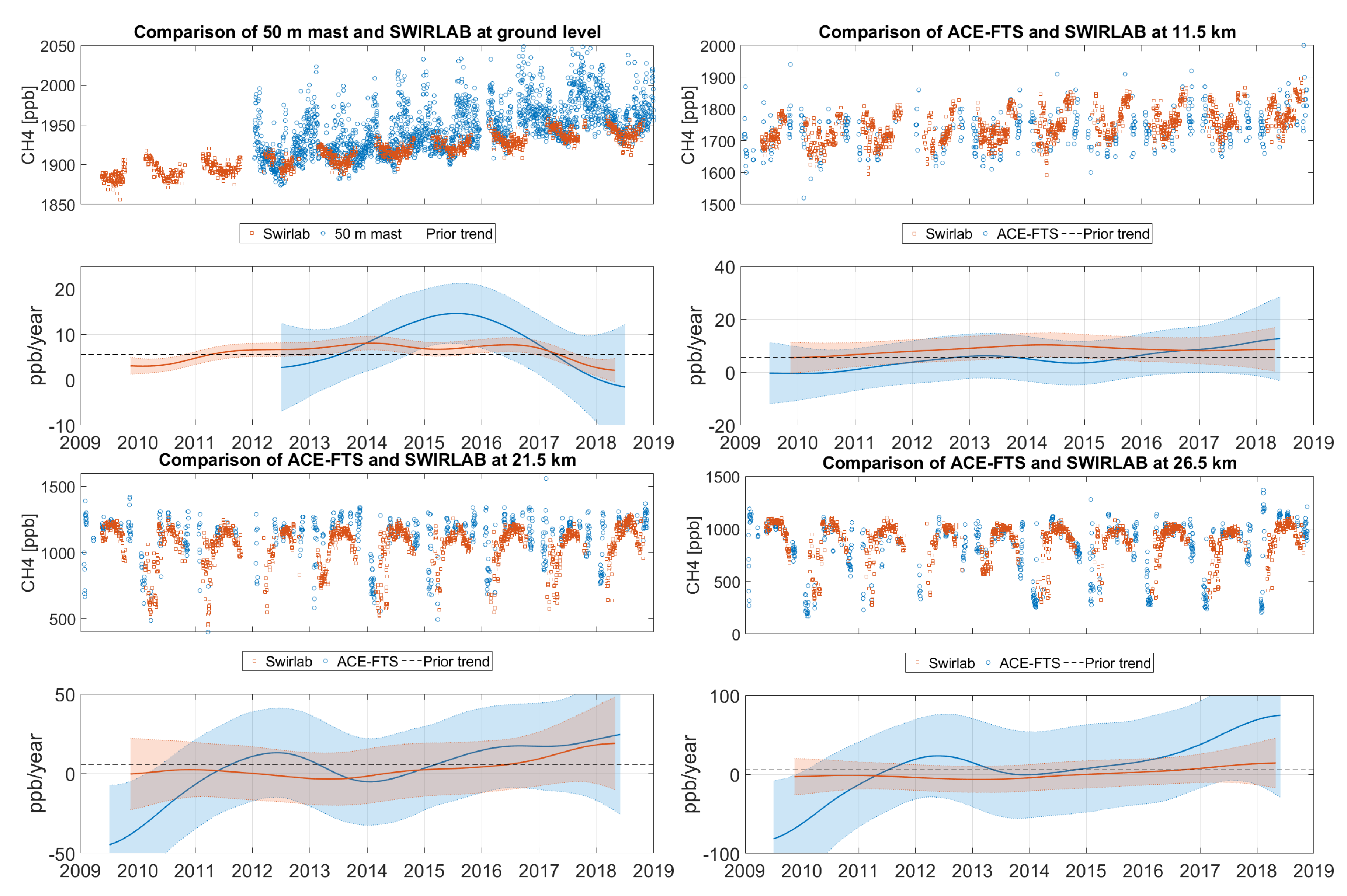
4.3. Profile Comparison to AirCore Measurements

The concurrent Swirlab and AirCore profiles are shown in Figure 10. The AirCore profiles were obtained during 2013–2017. During multiyear flights, all seasons have been represented. In 2017, the flights were performed within ESA FRM4GHG Project [47,48]. There is, in general, a good agreement between AirCore and Swirlab posterior profile. For some retrievals, another prior profile could have resulted in a better agreement. For example, on 24 and 26 April 2017, the polar vortex prior would follow the AirCore profiles more closely but the potential vorticity in the ECMWF data suggests Sodankylä was not inside the polar vortex so the winter prior profile is used. Nevertheless, the methane deficit in the stratosphere is quite well detected by Swirlab even when using the winter prior profile.

For quantitative analysis, we calculated the root mean square error (RMSE) of Swirlab retrievals against the AirCore profiles. The RMSE is defined as

$$\mathrm{RMSE}\left(x\right)={\left(\sum _{i=1}^N{(z_i-x_i)}^2/N\right)}^{\frac{1}{2}}$$

(24)

where x is the Swirlab profile, z is the AirCore profile and N is the number of layers where we have co-occurring data points. We performed the same RMSE analysis also for another set of profiles, retrieved using the prior scaling method from [32]. The prior scaling retrieval is similar to the one used in TCCON and thus serves as a good reference point. The results are presented in

Table 1. Root mean square errors of the posterior mean obtained by Swirlab profile retrieval and prior scaling method similar to the one used by TCCON, relative to the AirCore profile.

Date	AirCore-Swirlab	AirCore-Prior Scaling
3 September 2013	98.7	135.6
5 September 2013	188.4	259.5
22 October 2013	106.6	289.4
19 March 2014	61.1	46.3
9 April 2014	76.3	87.5
14 July 2014	81.4	61.9
15 July 2014	64.6	63.8
16 July 2014	60.9	53.6
2 September 2014	48.5	32.6
5 November 2014	158.5	222.9
14 April 2016	185.0	272.4
24 August 2016	65.5	43.7
21 April 2017	74.4	146.3
24 April 2017	167.3	384.5
26 April 2017	150.7	372.8
15 May 2017	54.1	97.8
28 August 2017	94.0	49.3
4 September 2017	40.3	44.1
5 September 2017	73.2	44.6
6 September 2017	41.0	28.4
7 September 2017	23.3	31.3
Mean	87.5	126.3

. We can conclude that, in the sense of RMSE, Swirlab tends to give results that are on average closer to the AirCore profile. In addition, looking at the measurements where the profile scaling yields a smaller RMSE than Swirlab, the differences between the methods are still relatively small. In contrast, in the majority of cases where Swirlab provided a better retrieval, it was significantly better. We would also like to note that, as can be seen in Figure 10, the retrievals where profile scaling performs better are generally times when the measured AirCore profile is very close to the prior profile.

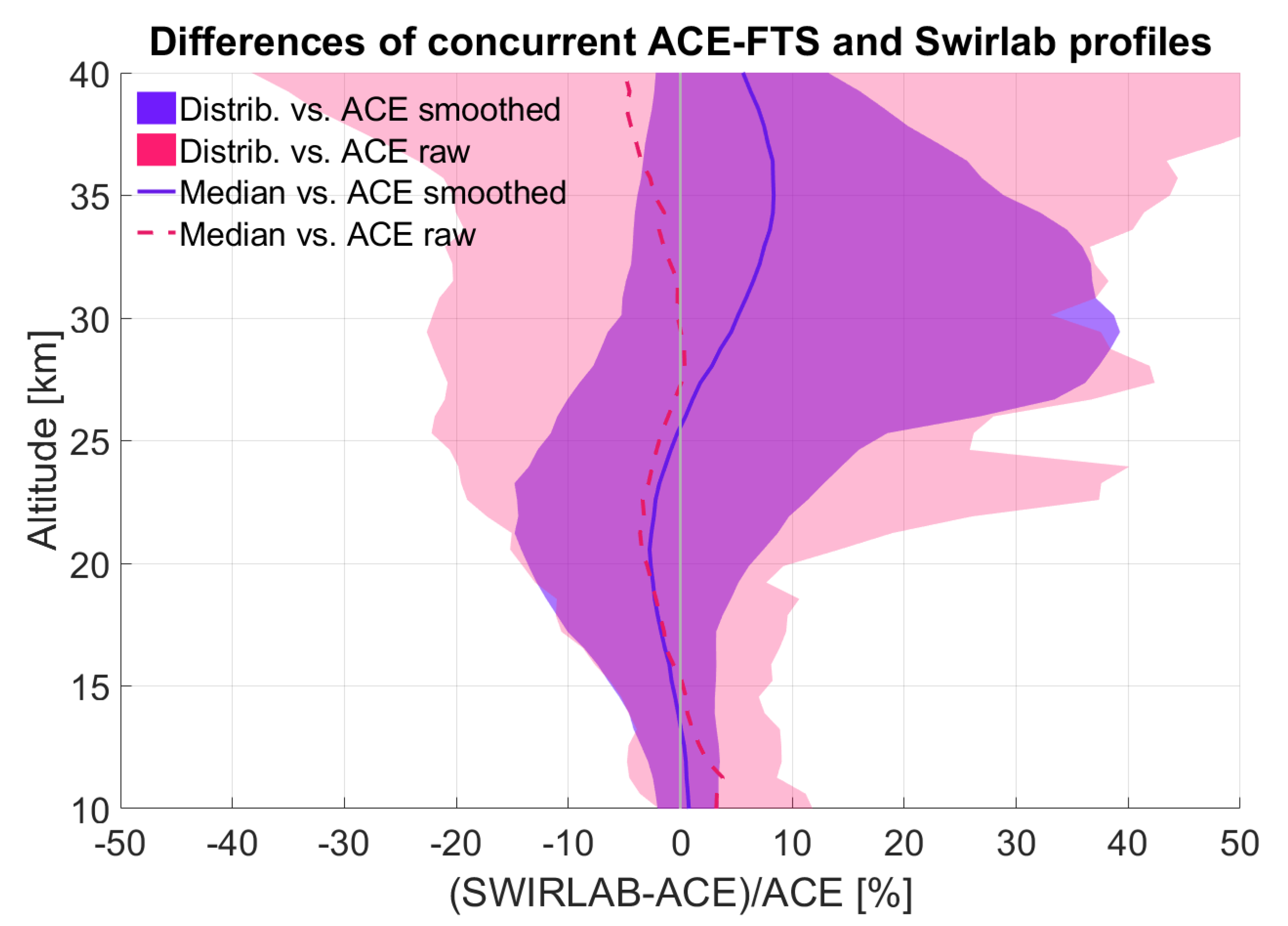
4.4. Profile Comparison with ACE-FTS Instrument

Swirlab retrievals were compared to both original and averaging kernel corrected ACE-FTS profiles (Figure 11). The comparison was made between the closest ACE-FTS retrieval of the day within the co-location region (see Figure 1) and the concurrent Swirlab retrieval over Sodankylä. For the averaging kernel correction, the missing values in ACE-FTS profiles have been filled with the Swirlab prior profile. The gap-filling method might partly explain the small negative bias below 25 km and small positive bias above 25 km when comparing averaging kernel corrected ACE-FTS to Swirlab.

A large set of ACE-FTS profiles was used to create the prior means for Swirlab and also the prior covariance was built to resemble the empirical covariance of ACE-FTS profiles. Therefore, it was expected that on average ACE-FTS and Swirlab would agree well. However, the information from ACE-FTS for the priors is condensed to three seasonal prior means. The variability around these priors, even if constrained to a realistic and smooth solution by the covariance, is interpreted from the spectra. In this regard, using ACE-FTS as a reference is justified.

The raw, non-smoothed, ACE-FTS profiles and Swirlab profiles agree well below 25 km with Swirlab retrievals staying within 25% from the satellite data. Between 25 and 35 km the profiles agree well on average but the variability becomes larger. The distribution of differences against non-smoothed ACE-FTS profiles is slightly asymmetric with the median difference being close to zero. The median suggests that there is an equal amount of cases where Swirlab concentrations are lower than cases where they are higher than ACE-FTS values. The asymmetry suggests that, when ACE values are lower, the discrepancies between the two retrievals are larger. This could be caused by Swirlab being unable to sense large methane deficits occurring on a limited altitude range that can occur close to the polar vortex edge when air from outside and inside the vortex are mixed [14]. Close to 40 km altitude, the Swirlab retrievals get closer to prior profiles and on average compare well with ACE-FTS but the variability ACE-FTS can detect is much larger than what is possible with Swirlab.

The Swirlab profiles compare well also to the averaging kernel corrected ACE-FTS profiles, the distribution of the differences resembling the comparison to raw ACE-FTS profiles but with slightly smaller variability. However, the asymmetry above 25 km is even larger than in the comparison with raw ACE-FTS. This again could also, at least partly, be caused by the gap-filling with the Swirlab prior information that might not represent the true profile. At levels close to 40 km, the variability becomes smaller as the sensitivity of Swirlab retrieval is reduced and the averaging kernel smoothed ACE-FTS profiles are forced closer to the prior profiles as are the Swirlab retrievals.

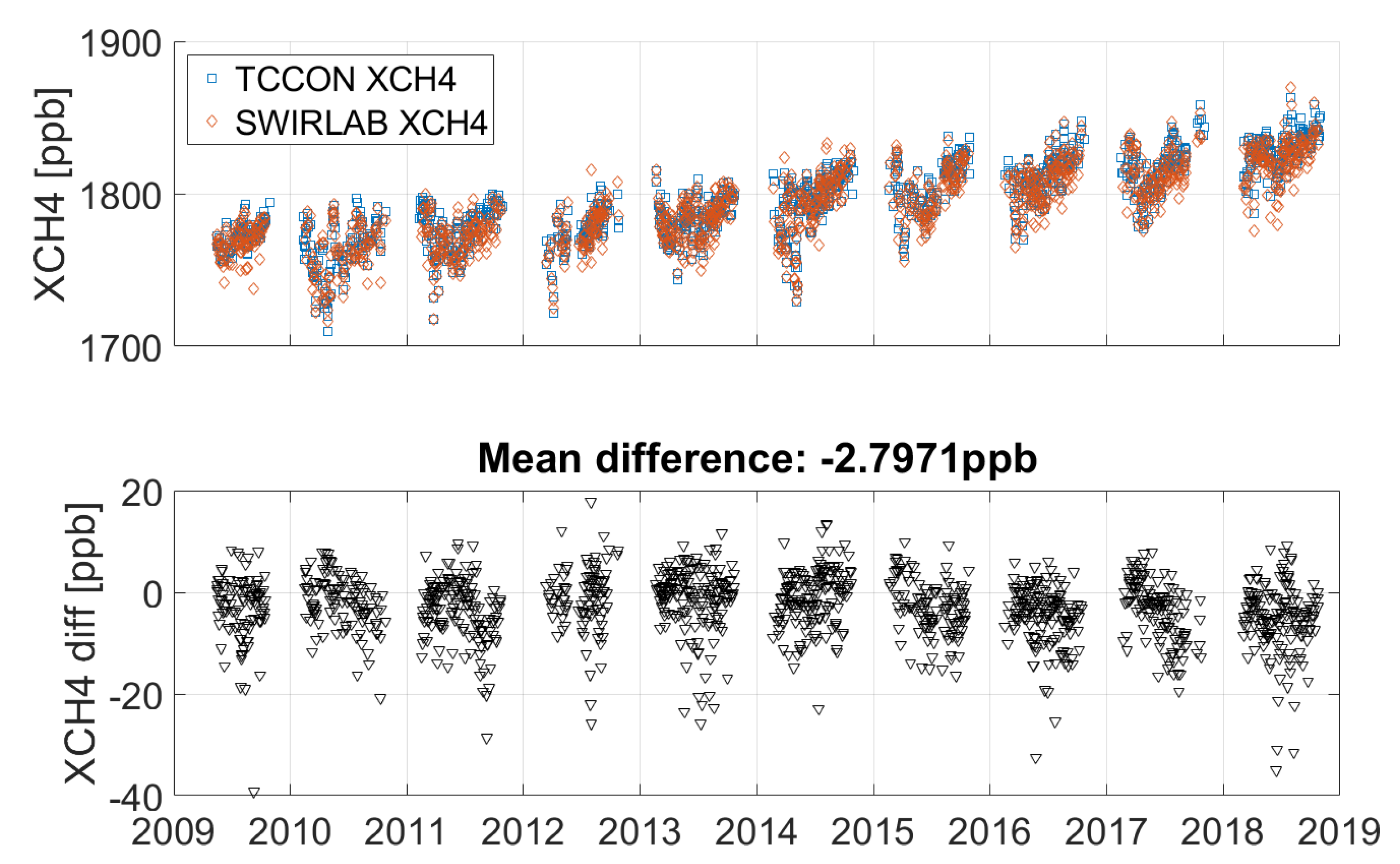
4.5. Total Column Comparison to the TCCON Algorithm

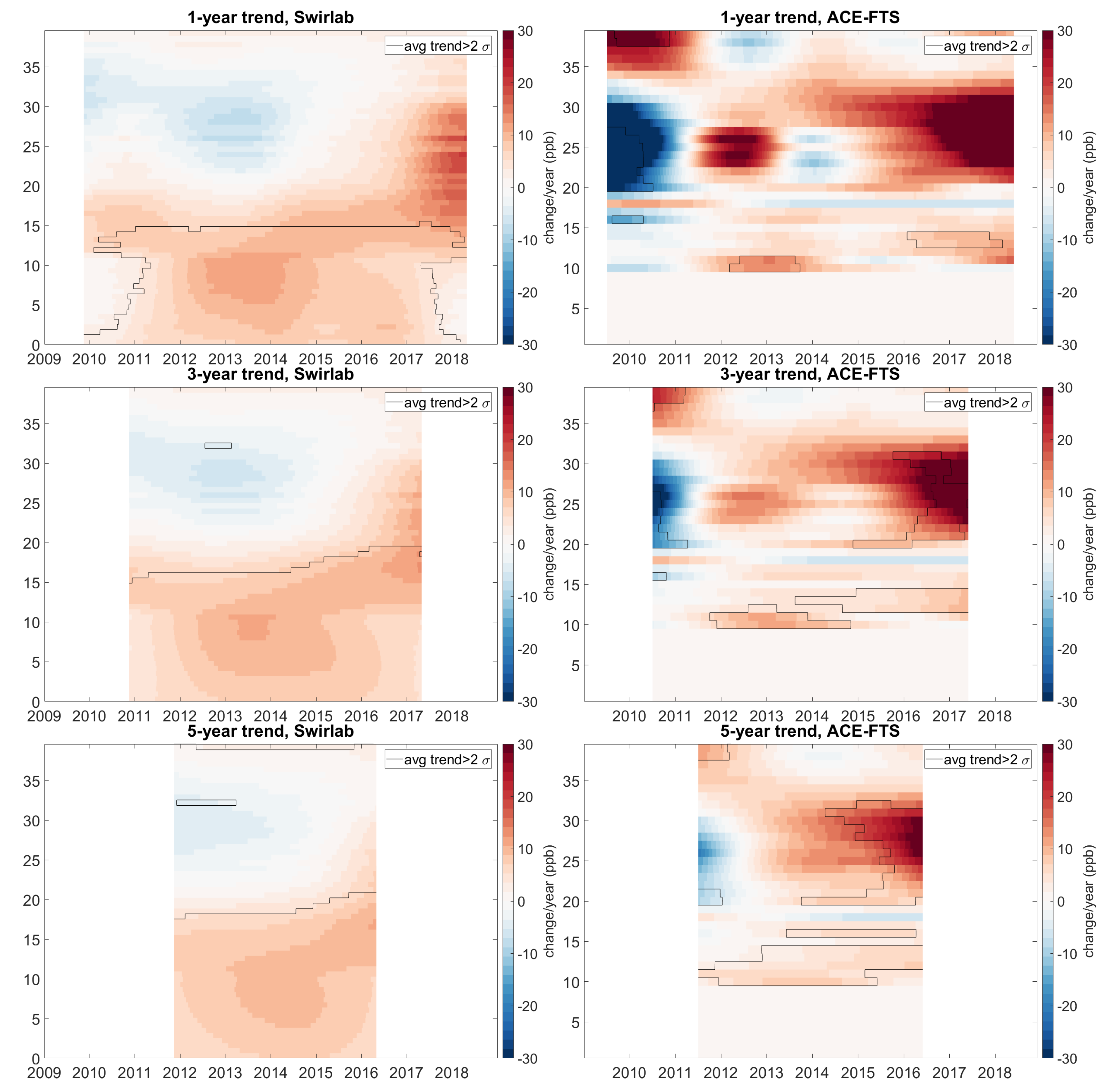
We used the pressure profile and water vapor profile from NCEP/NCAR data to calculate the total column dry air mole fraction (XCH${}_4$) from the Swirlab profiles. The daily averages of TCCON and Swirlab total columns are compared in Figure 12. The agreement is good with a mean bias of −2.8 ppb and standard deviation of 6.1 ppb. The trend of TCCON is followed well by Swirlab data, and based on the lack of seasonality in the residual time series, the SZA correction implemented to the Swirlab data is sufficient. A small step in the difference can be seen since the beginning of 2015 but its origin is unresolved.

The main difference of the two algorithms is the degree of freedom in finding the methane profile that would produce the measured spectra. TCCON scales the prior shape and Swirlab uses four singular vectors to modify also the shape of the profile. This improves the accuracy in cases where the prior profile significantly differs from the true profile. In addition, the residuals in the fit between the measured and modeled spectra become smaller as the absorption line shapes are allowed to vary [32].

There are also other differences. The wavelength range used by TCCON is wider as Swirlab uses one short microwindow (see Figure 2), whereas TCCON has three wavelength windows for its methane retrieval. The algorithms use slightly different absorption line data as Swirlab uses HITRAN2016 [42] and GGG2014 uses a modified HITRAN2012 [36]. Differences can also be partly attributed to the different way of defining the dry air column. As the Swirlab algorithm retrieves neither the O${}_2$ column nor the water vapor column, the dry air column used to derive the dry air mole fraction (DMF) is calculated from the NCEP/NCAR model data. In TCCON retrieval, the air column is calculated using the retrieved O${}_2$ column assuming that the DMF of oxygen is constant. The use of O${}_2$ column for air column estimation improves the precision as it reduces the effects of instrumental or measurement errors that are common to both gases CH${}_4$ and O${}_2$ [49].

4.6. Ch${}_4$ Trends

The CH${}_4$ profiles retrieved with Swirlab allow us to quantify the growth rate of atmospheric CH${}_4$ in every level during the 10-year time series. For this analysis, we drew samples from the posterior distribution of the level parameter ${\mu }_t$ in our DLM analysis. For each sample, we computed the yearly trend at a timestep t as a change

$${\mathrm{trend}}_t={\mu }_{t+s/2}-{\mu }_{t-s/2},$$

(25)

where s is the number of days considered. To assess the trend and the uncertainty, we drew 1000 samples and calculated the average trend and the standard deviation of the trend for every time step.

The Swirlab CH${}_4$ time series at four different levels (at the ground level, 11.5 km, 21.5 km and 26.5 km) and respective growth rates are shown in Figure 13. In the troposphere (upper panels in Figure 13; orange color), the results show a positive growth rate throughout the time series with moderate interannual variability, in particular at the ground level. The maximum growth rate of 8.1 ± 1.5 ppb/year occurs around winter 2013–2014 at the ground level, and also simultaneously higher in the troposphere. This is also clearly shown by Figure 14 (left panels), where the growth rate in all tropospheric levels increases until 2014, after which it begins to decrease but remains positive. It is notable that the growth rate has decreased significantly since 2017 at the ground level; however, this cannot be seen with confidence higher in the troposphere. The uncertainty estimates of the growth rate increase with altitude, as well as towards the edges of the time series. In the stratosphere (lower panels in Figure 13; orange color), the seasonal variability of CH${}_4$ is stronger, as well as the interannual variability; thus, weak trends are more challenging to quantify reliably. The variability of the growth rate is mostly smaller-scale than the estimated uncertainty range. The average stratospheric trend is estimated to be weak, and above roughly 20 km altitude, systematically weakly negative; however, the uncertainty estimates are large. Contrary to the ground level and the troposphere, the stratospheric CH${}_4$ growth rate based on Swirlab retrieval levels has been increasing since 2017 and even earlier in the lowest part of the stratosphere. In addition, the Swirlab data show a weak positive trend in the levels close to 40 km but at these high altitudes this is likely due to Swirlab retrieval closely following the prior with a predefined growth rate of 5.57 ppb/year.

We evaluated the Swirlab CH${}_4$ trend signatures described above through comparisons with appropriate reference data at different atmospheric levels. Figure 13 (upper left panel) shows a comparison of Swirlab to the 50-metre mast measurements. In general, the time series from the Swirlab retrieval agrees well with the in-situ measurements, albeit the local variability in the concentration is stronger for the mast measurements. The large variability of the in-situ data results in large uncertainty estimates for the growth rate, exceeding those of Swirlab. Both measurements agree that the trend is lower, almost zero, at the end of the time series, although the uncertainty also increases. For the overlapping time period 2012–2018, the estimated growth rate is 6.3 ± 0.4 ppb/year (the uncertainty denoting the 95% confidence interval) for Swirlab and 6.8 ± 2.6 ppb/year for the mast measurements.

At higher altitudes, the reference instrument is the ACE-FTS. As shown in Figure 13, the ACE-FTS and Swirlab time series agree well but the overall trends differ, although they are mostly within the uncertainty envelopes. As Swirlab is more constrained than ACE-FTS, the uncertainty estimates are larger for the latter. At 11.5 km, the eight-year trend from the beginning of 2010 until the end of 2017 (neglecting the edges of the DLM fit) shows a change of 4.9 ± 1.8 ppb/year in ACE-FTS measurements and 8.4 ± 1.2 ppb/year in Swirlab measurements. In the stratosphere, the ACE-FTS-derived growth rates are more subject to interannual variability. For the eight-year period of 2010–2017, overall, the trends at 21.5 km are 4.6 ± 4.8 ppb/year for ACE-FTS and 3.1 ± 3.4 ppb/year for Swirlab. At 26.5 km, the trends for the same period are 11.1 ± 11.0 ppb/year for ACE-FTS and −0.2 ± 4.4 ppb/year for Swirlab. The increasing growth rate towards the end of the ACE-FTS time series seems to be driven by the large increase from 2017 to 2018. This change is also noticeable in the Swirlab data albeit not as large as in the ACE-FTS data.

In Figure 14, the Swirlab growth rate is compared to that of the ACE-FTS at all levels and for different time scales. The ACE-FTS data are presented from 10 km upwards as the data are very sparse below that level. The analysis is also confined to the altitudes below 40 km as Swirlab is not very sensitive at altitudes above that and thus mostly follows the prior. Below 15 km, the instruments agree that there is a small but significant positive trend. However, between 15 and 20 km, ACE-FTS does not detect consistent growth while Swirlab does. From 20 to 35 km, Swirlab data show very stable methane concentrations with a weak yet insignificant negative trend until 2015 when the trend turns to weak positive, while ACE-FTS shows more variable trends in the beginning. In the latest years, Swirlab and ACE-FTS agree on a large but not statistically significant positive trend; however, in the ACE-FTS DLM fit, the trend is found significant in the three- and five-year time spans.

When comparing DLM trends for two datasets, it should be noted that the differences in concurrent measurements are not the only cause for differences in trends. The sampling of the data also has strong influence to the DLM fit. Random gaps in the data can create artifacts in the trends, especially if the measurement frequency is already sparse and the data gap hides a yearly maximum or minimum that is usually observed. Missing data in fall 2011 and early spring 2012 are partly the cause for the oscillations in the ACE-FTS stratospheric trends around winter 2011–2012. The larger amount of data in the Swirlab time series partially stabilizes the DLM fit but the missing values during the polar night make the fitting of the seasonal cycle challenging, as was also pointed out by Kivimäki et al. [50].

5. Discussion and Summary

We produced a ten-year time series of atmospheric methane profiles using a dimension reduction retrieval method to ground-based short wave infrared spectra measured with a Fourier Transform Spectrometer. After statistically correcting the solar zenith angle dependence, the retrieved profiles agree well with reference measurements: ACE-FTS above 10 km up to 40 km, AirCore from the surface to 25 km and 50-m mast air sampling measurements at the lowest altitude levels. The retrieval method succeeds in producing CH${}_4$ profiles with realistic trends and seasonal variability even when using a single prior throughout the time series but the comparison to reference instruments performs better when a prior trend assumption and seasonal prior profiles are introduced.

The DLM approach in the paper results in realistic trend estimates. Missing data, especially in the ACE-FTS time series with less frequent measurements over Sodankylä, can induce short-term variability. The data gap due to the polar night mostly influences the seasonal cycle fit rather than the trend.

The tropospheric trends in the Swirlab time series agree with the trend in local 50-m mast measurements. In a wider perspective, the weaker tropospheric trends until 2011 and higher trends after that agree with other Arctic stations reported by Nisbet et al. [18]. Interestingly, the weaker trend in the end of the time series from 2017 to 2018 does not follow the global average CH${}_4$ increase as reported by the Global Monitoring Division of NOAA’s Earth System Research Laboratory [51]; however, this weaker trend is shown by both mast measurements and Swirlab. The slowdown of the growth rate could be interpreted as: (1) the decrease of surface fluxes in the influencing areas of the mast; (2) decreased biomass signals from e.g., Siberia; and (3) a transport pattern change. However, confirming the reason demands a thorough model study outside the scope of this work and thus can only be speculated here.

In the stratosphere, the CH${}_4$ growth rates from ACE-FTS and Swirlab retrievals are generally in a good agreement. However, the confidence limits of the trend are larger than in the troposphere because of a larger uncertainty of the retrieved values, and a larger seasonal and interannual variability in the methane concentrations. Therefore, to be reliably detected from other variability, the growth rate would need to be consistent over a long time period. The significance of the estimated growth rate was evaluated by its deviation from zero with 95% confidence. As shown in Figure 14, both instruments detect mostly insignificant changes in the stratospheric CH${}_4$ over Sodankylä. However, in the ACE-FTS time series, the positive stratospheric trends towards the end of the time series are found to be significant, contrary to the trends estimated for Swirlab. This could originate from higher vertical resolution of ACE-FTS but could also be caused by the differences in the DLM fitting due to less frequent data points in the ACE-FTS time series.

Albeit appearing towards the edge of the time series, the rising stratospheric trend from 2017 to 2018 draws attention. There is a slight suspicion that this could be an edge effect in the DLM fit, especially as there is a similar negative trend in the beginning of the time series. However, the late rise can be identified in both ACE-FTS and Swirlab data at the 26.5 km altitude as a high, sudden increase in CH${}_4$ from 2017 to 2018, suggesting that the DLM-inferred positive trends are indeed described by the data. The stratospheric air at high latitudes mostly originates from the tropical troposphere. Therefore, the stratospheric methane concentrations in the Arctic are not expected to follow the changes in the local troposphere: the stratospheric air may have been transported several years after being in contact with methane sources at the surface. Hence, the recent sudden increase of CH${}_4$ in the Arctic stratosphere could point to enhanced circulation from the tropics or to a decrease in stratospheric methane sink. However, continuing observations are needed to confirm and monitor this increase, and further studies involving atmospheric inverse modeling are necessary for pinpointing the reason for the observed growth rate.

Overall, the method discussed in this paper is a valuable addition to other methane profile measurements. While it does not reach the accuracy and vertical resolution of aircraft and balloon-borne measurements, the temporal coverage is much better. The information provided by the method will be a valuable addition to the existing continuous monitoring of the total column and the surface concentrations of methane. These continuous measurements can further help to develop models and reliably track the changes in the sources and sinks of methane. In this work, we considered a local scale but the method is publicly available and applicable to any ground-based, high-resolution spectrometer measuring in the short-wave infrared wavelength range.

References

1. Myhre, G.; Shindell, D.; Bréon, F.M.; Collins, W.; Fuglestvedt, J.; Huang, J.; Koch, D.; Lamarque, J.F.; Lee, D.; Mendoza, B.; et al. Anthropogenic and natural radiative forcing. In Climate Change 2013: The Physical Science Basis; Contribution of Working Group I to the Fifth Assessment Report of the Intergovernmental Panel on Climate Change; Stocker, T.F., Qin, D., Plattner, G.K., Tignor, M., Allen, S.K., Doschung, J., Nauels, A., Xia, Y., Bex, V., Midgley, P.M., Eds.; Cambridge University Press: Cambridge, UK, 2013; pp. 659–740. [Google Scholar] [CrossRef]
2. Prather, M.J.; Holmes, C.D.; Hsu, J. Reactive greenhouse gas scenarios: Systematic exploration of uncertainties and the role of atmospheric chemistry. Geophys. Res. Lett. 2012, 39. [Google Scholar] [CrossRef] [Green Version]
3. Etheridge, D.M.; Steele, L.P.; Francey, R.J.; Langenfelds, R.L. Atmospheric methane between 1000 A.D. and present: Evidence of anthropogenic emissions and climatic variability. J. Geophys. Res. Atmos. 1998, 103, 15979–15993. [Google Scholar] [CrossRef]
4. Dlugokencky, E.J.; Crotwell, A.M.; Mund, J.W.; Crotwell, M.J.; Thoning, K.W. Atmospheric Methane Dry Air Mole Fractions from the NOAA ESRL Carbon Cycle Cooperative Global Air Sampling Network; ESRL/GMD CCGG Group: Boulder, CO, USA, 2019. [CrossRef]
5. Saunois, M.; Stavert, A.R.; Poulter, B.; Bousquet, P.; Canadell, J.G.; Jackson, R.B.; Raymond, P.A.; Dlugokencky, E.J.; Houweling, S.; Patra, P.K.; et al. The Global Methane Budget 2000–2017. Earth Syst. Sci. Data Discuss. 2019, 2019, 1–136. [Google Scholar] [CrossRef]
6. Dean, J.F.; Middelburg, J.J.; Röckmann, T.; Aerts, R.; Blauw, L.G.; Egger, M.; Jetten, M.S.; de Jong, A.E.; Meisel, O.H.; Rasigraf, O.; et al. Methane Feedbacks to the Global Climate System in a Warmer World. Rev. Geophys. 2018, 56, 207–250. [Google Scholar] [CrossRef]
7. Worthy, D.; Taylor, C.; Dlugokencky, E.; Chan, E.; Nisbet, E.G.; Laurila, T. Long-Term Monitoring of Atmospheric Methane; Arctic Monitoring and Assessment Programme (AMAP): Oslo, Norway, 2015; Chapter 6; pp. 61–75. [Google Scholar]
8. Thanwerdas, J.; Saunois, M.; Berchet, A.; Pison, I.; Hauglustaine, D.; Ramonet, M.; Crevoisier, C.; Baier, B.; Sweeney, C.; Bousquet, P. C:12 C isotopic ratio at global scale. Atmos. Chem. Phys. Discuss. 2019, 1–28. [Google Scholar] [CrossRef] [Green Version]
9. Bruhwiler, L.M.; Basu, S.; Bergamaschi, P.; Bousquet, P.; Dlugokencky, E.; Houweling, S.; Ishizawa, M.; Kim, H.S.; Locatelli, R.; Maksyutov, S.; et al. CH4 emissions from oil and gas production: Have recent large increases been detected? J. Geophys. Res. 2017, 122, 4070–4083. [Google Scholar] [CrossRef] [Green Version]
10. Sasakawa, M.; Machida, T.; Ishijima, K.; Arshinov, M.; Patra, P.K.; Ito, A.; Aoki, S.; Petrov, V. Temporal Characteristics of CH4 Vertical Profiles Observed in the West Siberian Lowland Over Surgut From 1993 to 2015 and Novosibirsk From 1997 to 2015. J. Geophys. Res. Atmos. 2017, 122, 11261–11273. [Google Scholar] [CrossRef]
11. Brewer, A.W. Evidence for a world circulation provided by the measurements of helium and water vapour distribution in the stratosphere. Q. J. R. Meteorol. Soc. 1949, 75, 351–363. [Google Scholar] [CrossRef]
12. Holton, J.R.; Haynes, P.H.; McIntyre, M.E.; Douglass, A.R.; Rood, R.B.; Pfister, L. Stratosphere-troposphere exchange. Rev. Geophys. 1995, 33, 403–439. [Google Scholar] [CrossRef]
13. Schoeberl, M.R.; Hartmann, D.L. The dynamics of the stratospheric polar vortex and its relation to springtime ozone depletions. Science 1991, 251, 46–52. [Google Scholar] [CrossRef] [Green Version]
14. Röckmann, T.; Brass, M.; Borchers, R.; Engel, A. The isotopic composition of methane in the stratosphere: High-altitude balloon sample measurements. Atmos. Chem. Phys. 2011, 11, 13287–13304. [Google Scholar] [CrossRef] [Green Version]
15. Dlugokencky, E.J.; Houweling, S.; Bruhwiler, L.; Masarie, K.A.; Lang, P.M.; Miller, J.B.; Tans, P.P. Atmospheric methane levels off: Temporary pause or a new steady-state? Geophys. Res. Lett. 2003, 30, 3–6. [Google Scholar] [CrossRef] [Green Version]
16. Nisbet, E.G.; Dlugokencky, E.J.; Manning, M.R.; Lowry, D.; Fisher, R.E.; France, J.L.; Michel, S.E.; Miller, J.B.; White, J.W.; Vaughn, B.; et al. Rising atmospheric methane: 2007–2014 growth and isotopic shift. Glob. Biogeochem. Cycles 2016. [Google Scholar] [CrossRef] [Green Version]
17. Rigby, M.; Montzka, S.A.; Prinn, R.G.; White, J.W.C.; Young, D.; O’Doherty, S.; Lunt, M.F.; Ganesan, A.L.; Manning, A.J.; Simmonds, P.G.; et al. Role of atmospheric oxidation in recent methane growth. Proc. Natl. Acad. Sci. USA 2017, 114, 5373–5377. [Google Scholar] [CrossRef] [PubMed] [Green Version]
18. Nisbet, E.G.; Manning, M.R.; Dlugokencky, E.J.; Fisher, R.E.; Lowry, D.; Michel, S.E.; Myhre, C.L.; Platt, S.M.; Allen, G.; Bousquet, P.; et al. Very Strong Atmospheric Methane Growth in the 4 Years 2014–2017: Implications for the Paris Agreement. Glob. Biogeochem. Cycles 2019, 33, 318–342. [Google Scholar] [CrossRef]
19. Steele, L.P.; Fraser, P.J.; Rasmussen, R.A.; Khalil, M.A.K.; Conway, T.J.; Crawford, A.J.; Gammon, R.H.; Masarie, K.A.; Thoning, K.W. The global distribution of methane in the troposphere. J. Atmos. Chem. 1987, 5, 125–171. [Google Scholar] [CrossRef]
20. Dlugokencky, E.J.; Steele, L.P.; Lang, P.M.; Masarie, K.A. The growth rate and distribution of atmospheric methane. J. Geophys. Res. 1994, 99, 17021–17043. [Google Scholar] [CrossRef]
21. Wunch, D.; Toon, G.C.; Blavier, J.F.L.; Washenfelder, R.A.; Notholt, J.; Connor, B.J.; Griffith, D.W.T.; Sherlock, V.; Wennberg, P.O. The Total Carbon Column Observing Network. Philos. Trans. R. Soc. Lond. A Math. Phys. Eng. Sci. 2011, 369, 2087–2112. [Google Scholar] [CrossRef] [Green Version]
22. De Mazière, M.; Thompson, A.M.; Kurylo, M.J.; Wild, J.D.; Bernhard, G.; Blumenstock, T.; Braathen, G.O.; Hannigan, J.W.; Lambert, J.C.; Leblanc, T.; et al. The Network for the Detection of Atmospheric Composition Change (NDACC): History, status and perspectives. Atmos. Chem. Phys. 2018, 18, 4935–4964. [Google Scholar] [CrossRef] [Green Version]
23. Hu, H.; Hasekamp, O.; Butz, A.; Galli, A.; Landgraf, J.; Aan de Brugh, J.; Borsdorff, T.; Scheepmaker, R.; Aben, I. The operational methane retrieval algorithm for TROPOMI. Atmos. Meas. Tech. 2016, 9, 5423–5440. [Google Scholar] [CrossRef] [Green Version]
24. Parker, R.; Boesch, H.; Cogan, A.; Fraser, A.; Feng, L.; Palmer, P.I.; Messerschmidt, J.; Deutscher, N.; Griffith, D.W.T.; Notholt, J.; et al. Methane observations from the Greenhouse Gases Observing SATellite: Comparison to ground-based TCCON data and model calculations. Geophys. Res. Lett. 2011, 38. [Google Scholar] [CrossRef] [Green Version]
25. Karion, A.; Sweeney, C.; Tans, P.; Newberger, T. AirCore: An Innovative Atmospheric Sampling System. J. Atmos. Ocean. Technol. 2010, 27, 1839–1853. [Google Scholar] [CrossRef]
26. Verma, S.; Marshall, J.; Parrington, M.; Agustí-Panareda, A.; Massart, S.; Chipperfield, M.P.; Wilson, C.; Gerbig, C. Extending methane profiles from aircraft into the stratosphere for satellite total column validation using the ECMWF C-IFS and TOMCAT/SLIMCAT 3-D model. Atmos. Chem. Phys. 2017, 17, 6663–6678. [Google Scholar] [CrossRef] [Green Version]
27. Tukiainen, S. Swirlab. Available online: https://github.com/tukiains/swirlab (accessed on 2 August 2019).
28. Hase, F.; Hannigan, J.; Coffey, M.; Goldman, A.; Höpfner, M.; Jones, N.; Rinsland, C.; Wood, S. Intercomparison of retrieval codes used for the analysis of high-resolution, ground-based FTIR measurements. J. Quant. Spectrosc. Radiat. Transf. 2004, 87, 25–52. [Google Scholar] [CrossRef]
29. Zhou, M.; Langerock, B.; Sha, M.K.; Kumps, N.; Hermans, C.; Petri, C.; Warneke, T.; Chen, H.; Metzger, J.M.; Kivi, R.; et al. Retrieval of atmospheric CH4 vertical information from ground-based FTS near-infrared spectra. Atmos. Meas. Tech. 2019, 12, 6125–6141. [Google Scholar] [CrossRef]
30. Mueller, J.; Siltanen, S. Linear and Nonlinear Inverse Problems with Practical Applications; Society for Industrial and Applied Mathematics: Philadelphia, PA, USA, 2012. [Google Scholar]
31. Solonen, A.; Cui, T.; Hakkarainen, J.; Marzouk, Y. On dimension reduction in Gaussian filters. Inverse Problems 2016, 32, 045003. [Google Scholar] [CrossRef] [Green Version]
32. Tukiainen, S.; Railo, J.; Laine, M.; Hakkarainen, J.; Kivi, R.; Heikkinen, P.; Chen, H.; Tamminen, J. Retrieval of atmospheric CH4 profiles from Fourier transform infrared data using dimension reduction and MCMC. J. Geophys. Res. Atmos. 2016, 121, 10312–10327, 2015JD024657. [Google Scholar] [CrossRef] [Green Version]
33. Laine, M. Introduction to Dynamic Linear Models for Time Series Analysis. In Geodetic Time Series Analysis in Earth Sciences; Montillet, J.P., Bos, M., Eds.; Springer: Berlin, Germany, 2019; pp. 139–156. [Google Scholar] [CrossRef] [Green Version]
34. Kivi, R.; Heikkinen, P. Fourier transform spectrometer measurements of column CO2 at Sodankylä, Finland. Geosci. Instrum. Methods Data Syst. 2016, 5, 271–279. [Google Scholar] [CrossRef] [Green Version]
35. Wunch, D.; Toon, G.C.; Sherlock, V.; Deutscher, N.M.; Liu, C.; Feist, D.G.; Wennberg, P.O. The Total Carbon Column Observing Network’s GGG2014 Data Version; The Total Carbon Column Observing Network (TCCON); 2015; Available online: https://data.caltech.edu/records/249 (accessed on 8 August 2019). [CrossRef]
36. Rothman, L.; Gordon, I.; Babikov, Y.; Barbe, A.; Benner, D.C.; Bernath, P.; Birk, M.; Bizzocchi, L.; Boudon, V.; Brown, L.; et al. The HITRAN2012 molecular spectroscopic database. J. Quant. Spectrosc. Radiat. Transf. 2013, 130, 4–50. [Google Scholar] [CrossRef]
37. Kivi, R.; Heikkinen, P.; Kyrö, E. TCCON Data from Sodankylä (FI), Release GGG2014.R0. 2017. Available online: https://data.caltech.edu/records/289 (accessed on 28 June 2019). [CrossRef]
38. Bernath, P.F.; McElroy, C.T.; Abrams, M.C.; Boone, C.D.; Butler, M.; Camy-Peyret, C.; Carleer, M.; Clerbaux, C.; Coheur, P.F.; Colin, R.; et al. Atmospheric chemistry experiment (ACE): Mission overview. Geophys. Res. Lett. 2005, 32, 1–5. [Google Scholar] [CrossRef]
39. De Mazière, M.; Vigouroux, C.; Bernath, P.F.; Baron, P.; Blumenstock, T.; Boone, C.; Brogniez, C.; Catoire, V.; Coffey, M.; Duchatelet, P.; et al. Validation of ACE-FTS v2.2 methane profiles from the upper troposphere to the lower mesosphere. Atmos. Chem. Phys. 2008, 8, 2421–2435. [Google Scholar] [CrossRef] [Green Version]
40. Chen, H.; Winderlich, J.; Gerbig, C.; Hoefer, A.; Rella, C.W.; Crosson, E.R.; Van Pelt, A.D.; Steinbach, J.; Kolle, O.; Beck, V.; et al. High-accuracy continuous airborne measurements of greenhouse gases (CO2 and CH4) using the cavity ring-down spectroscopy (CRDS) technique. Atmos. Meas. Tech. 2010, 3, 375–386. [Google Scholar] [CrossRef] [Green Version]
41. Rella, C.W.; Chen, H.; Andrews, A.E.; Filges, A.; Gerbig, C.; Hatakka, J.; Karion, A.; Miles, N.L.; Richardson, S.J.; Steinbacher, M.; et al. High accuracy measurements of dry mole fractions of carbon dioxide and methane in humid air. Atmos. Meas. Tech. 2013, 6, 837–860. [Google Scholar] [CrossRef] [Green Version]
42. Gordon, I.E.; Rothman, L.S.; Hill, C.; Kochanov, R.V.; Tan, Y.; Bernath, P.F.; Birk, M.; Boudon, V.; Campargue, A.; Chance, K.V.; et al. The HITRAN2016 molecular spectroscopic database. J. Quant. Spectrosc. Radiat. Transf. 2017, 203, 3–69. [Google Scholar] [CrossRef]
43. Marzouk, Y.M.; Najm, H.N. Dimensionality reduction and polynomial chaos acceleration of Bayesian inference in inverse problems. J. Comput. Phys. 2009, 228, 1862–1902. [Google Scholar] [CrossRef] [Green Version]
44. Rodgers, C.D.; Connor, B.J. Intercomparison of remote sounding instruments. J. Geophys. Res. 2003, 108. [Google Scholar] [CrossRef] [Green Version]
45. Laine, M.; Latva-Pukkila, N.; Kyrölä, E. Analysing time-varying trends in stratospheric ozone time series using the state space approach. Atmos. Chem. Phys. 2014, 14, 9707–9725. [Google Scholar] [CrossRef] [Green Version]
46. Laine, M. DLM Toolbox for Matlab. Available online: https://mjlaine.github.io/dlm/ (accessed on 8 July 2019).
47. Sha, M.K.; De Mazière, M.; Notholt, J.; Blumenstock, T.; Chen, H.; Griffith, D.; Hase, F.; Heikkinen, P.; Hoffmann, A.; Huebner, M.; et al. FRM4GHG level2 dataset from the Sodankylä campaign. 2019. Available online: http://frm4ghg.aeronomie.be/index.php/outreach/datasetlevel2doi (accessed on 18 November 2019). [CrossRef]
48. Sha, M.K.; De Mazière, M.; Notholt, J.; Blumenstock, T.; Chen, H.; Dehn, A.; Griffith, D.W.T.; Hase, F.; Heikkinen, P.; Hermans, C.; et al. Intercomparison of low and high resolution infrared spectrometers for ground-based solar remote sensing measurements of total column concentrations of CO2, CH4 and CO. Atmos. Meas. Tech. Discuss. 2019, 2019, 1–67. [Google Scholar] [CrossRef] [Green Version]
49. Wunch, D.; Toon, G.C.; Wennberg, P.O.; Wofsy, S.C.; Stephens, B.B.; Fischer, M.L.; Uchino, O.; Abshire, J.B.; Bernath, P.; Biraud, S.C.; et al. Calibration of the total carbon column observing network using aircraft profile data. Atmos. Meas. Tech. 2010, 3, 1351–1362. [Google Scholar] [CrossRef] [Green Version]
50. Kivimäki, E.; Lindqvist, H.; Hakkarainen, J.; Laine, M.; Sussmann, R.; Tsuruta, A.; Detmers, R.; Deutscher, N.M.; Dlugokencky, E.J.; Hase, F.; et al. Evaluation and Analysis of the Seasonal Cycle and Variability of the Trend from GOSAT Methane Retrievals. Remote Sens. 2019, 11, 882. [Google Scholar] [CrossRef] [Green Version]
51. Dlugokencky, E. NOAA/ESRL Trends in Atmospheric Methane. Available online: https://www.esrl.noaa.gov/gmd/ccgg/trends_ch4/ (accessed on 20 January 2020).
Figure 1. Sodankylä (67.367 ° N, 26.629 ° E) marked with a star and the co-location criteria (3 ° in latitude, 30 ° in longitude) for ACE-FTS satellite measurements marked with dark rectangle.
Remotesensing 12 00917 g001
Figure 2. An example spectrum measured using ground-based Fourier Transform Spectrometer at noon on 20 June 2016. The figure covers the wavenumber range used in the Swirlab profile retrieval including strong and weak CH 4 absorbing features.
Remotesensing 12 00917 g002
Figure 3. The shapes of the three seasonally selected prior mean profiles. Summer profile is used from May to August and the polar vortex profile when potential vorticity exceeds a threshold value. For the rest of the cases, winter prior profile is used.
Remotesensing 12 00917 g003
Figure 4. (left) Visualization of the prior covariance structure used for the retrieval. (right) The first four singular vectors calculated from the prior covariance matrix.
Remotesensing 12 00917 g004
Figure 5. (top left) Dependence of the methane mixing ratio on solar zenith angle for the layer with the center altitude of 0.3 km. (top right) Dependence of the methane mixing ratio on solar zenith angle for the layer with the center altitude of 21.9 km. (bottom left) The SZA correction fits color coded for each layer. (bottom right) The interquartile range of the data points’ distance to the fitted curve depicted as a color plot for each layer.
Remotesensing 12 00917 g005
Figure 6. Every fifth layer of a full Swirlab kernel matrix at SZA = 45 ° depicted in ppb units. This describes how a change at a given altitude, color coded on the right, propagates to other altitudes in the retrieval.
Remotesensing 12 00917 g006
Figure 7. Swirlab time series. Each daily average profile is drawn as one column with the volume mixing ratio of methane depicted with a color. Data gaps shorter than seven days have been filled using the previous existing daily average profile.
Remotesensing 12 00917 g007
Figure 8. The effect of seasonal prior profile in the stratosphere (26.5 km), where the seasonal variability is the largest. The red squares represent Swirlab retrievals using seasonal priors. Yellow diamonds show the Swirlab time series when a single prior profile shape is used throughout the time series, however including a trend of 5.57 ppb/year. Blue circles show the ACE-FTS data used as a reference.
Remotesensing 12 00917 g008
Figure 9. Difference between the total columns calculated from the Swirlab profiles when the retrieval is made including or neglecting the trend in the prior profile.
Remotesensing 12 00917 g009
Figure 10. Comparison between Swirlab and AirCore methane profiles. The altitudes on the vertical axes are in kilometers (km) and the concentrations on horizontal axes in parts per billion (ppb). Red lines are the AirCore profiles. Black dashed line is the prior profile with prior variance in grey shading. Blue dotted line is the posterior mean with blue shading representing the 95% posterior.
Remotesensing 12 00917 g010
Figure 11. Median differences between daily average profiles from ACE-FTS and Swirlab. The curtain plots show 95th percentile of comparison between ACE-FTS profiles and Swirlab profiles. ACE smoothed has been averaging kernel corrected as described in Section 3.2.
Remotesensing 12 00917 g011
Figure 12. Comparison of total methane column calculated form Swirlab profiles against the total column from official TCCON GGG2014 product. (top panel) The daily averages of both retrievals. (bottom panel) The difference between Swirlab and TCCON.
Remotesensing 12 00917 g012
Figure 13. (top left) The lowest layer of Swirlab retrieval compared against 50-m mast measurements. (top right) Swirlab compared to ACE-FTS instrument at 11.5 km. (bottom left) Swirlab compared to ACE-FTS instrument at 21.5 km. (bottom right) Swirlab compared to ACE-FTS instrument at 26.5 km. For every altitude, the upper axis shows the daily averages from compared instruments and the lower axis shows the one-year average trend and the 95% confidence limits evaluated from the DLM analysis. Swirlab data are in orange and the reference instrument in blue. The dashed black line shows the Swirlab prior trend.
Remotesensing 12 00917 g013
Figure 14. Surface plots of DLM trends at altitudes from 0 to 40 km based on two different methods: Swirlab retrieval using ground-based remote sensing and ACE-FTS retrieval using satellite-based solar occultation measurements. Swirlab trends are on the left and ACE-FTS trends on the right. The top row shows trends calculated for change over a one-year period, the middle row for a three-year range and the bottom row for a five-year range. The black line confines the areas where the trend differs from zero with a 95% confidence level.
Remotesensing 12 00917 g014