Recurrence Analysis of Vegetation Indices for Highlighting the Ecosystem Response to Drought Events: An Application to the Amazon Forest

Abstract

Forests are important in sequestering CO₂ and therefore play a significant role in climate change. However, the CO₂ cycle is conditioned by drought events that alter the rate of photosynthesis, which is the principal physiological action of plants in transforming CO₂ into biological energy. This study applied recurrence quantification analysis (RQA) to describe the evolution of photosynthesis-related indices to highlight disturbance alterations produced by the Atlantic Multidecadal Oscillation (AMO, years 2005 and 2010) and the El Niño-Southern Oscillation (ENSO, year 2015) in the Amazon forest. The analysis was carried out using Moderate Resolution Imaging Spectroradiometer (MODIS) images to build time series of the enhanced vegetation index (EVI), the normalized difference water index (NDWI), and the land surface temperature (LST) covering the period 2001–2018. The results did not show significant variations produced by AMO throughout the study area, while a disruption due to the global warming phase linked to the extreme ENSO event occurred, and the forest was able to recover. In addition, spatial differences in the response of the forest to the ENSO event were found. These findings show that the application of RQA to the time series of vegetation indices supports the evaluation of the forest ecosystem response to disruptive events. This approach provides information on the capacity of the forest to recover after a disruptive event and, therefore is useful to estimate the resilience of this particular ecosystem.

1. Introduction

Terrestrial ecosystems such as forests absorb approximately 60 Gt of carbon annually [1]. Simultaneously, autotrophic and heterotrophic organisms release approximately the same amount of carbon back into the atmosphere, thus closing the terrestrial carbon cycle. Small alterations in the terrestrial carbon budget are likely to have a significant impact on atmospheric CO₂ concentrations [2,3]. There has been substantial warming in the northern high latitudes, which has been associated with changes in the inter-annual variability of the global carbon cycle [4,5]. Documenting and interpreting changes in the ecosystem functions that influence the carbon cycle globally is critical for understanding the associations and feedback between temperature, land cover, and atmospheric CO₂ [6,7].

Plants and other organisms that convert light energy into chemical energy in photosynthesis, are key in the terrestrial carbon cycle, particularly in territories in which ecosystem forests represent large portions of the area [8]. As a result of photosynthesis, the energy fluxes from the Sun to the Earth can be transformed and used to support life. It is thus considered the basis for all ecosystem services: food, fiber, fuel, etc. [9,10,11,12,13,14].

At a global scale, the monitoring of the pattern of photosynthesis of the mainly forest ecosystem can be useful to describe the overall changes in the vegetation vigor and energy flows. It is thus important to analyze the ability of terrestrial ecosystems to support photosynthetic activity and how such ecological functions can be altered and respond to external disturbance agents [15]. Each ecosystem pattern is characterized by the specific recurrence of photosynthesis cycles that present periodic or non-periodic and regularity patterns at different time scales [16]. The pattern of the photosynthesis is influenced by external inputs such as climate conditions and anthropogenic activities, which act at different spatial and temporal scales [17,18].

The Amazon is the largest tropical forest in the world and currently represents half of the tropical forest carbon stocks [19]. Small variations in the photosynthesis of the forest can substantially affect the CO₂ budget in the atmosphere, with impacts on climate changes at both the global and local scales [19,20,21,22]. In the last 25 years, the Amazon forest has been subjected to strong drought events and there is scientific debate regarding the effects on the carbon cycle [23,24]. In fact, these events have led to water deficits with the possible death of individual trees, producing changes in the forest canopy structure and functions [20,23,25,26,27].

The canopy structure of the forests affects the carbon dynamics of an ecosystem by influencing photosynthetic activities including recruitment, growth, and mortality. However, the exact nature of this effect is not well known [28]. A key parameter in determining the magnitude of this effect is the sensitivity or resilience of tropical forests to drought [20]. Ecological resilience is the capacity of the ecosystems to absorb or withstand perturbations or disturbances, recovering quickly and maintaining its structure and functions [29,30]. Thus, methods are required that highlight and describe the variations in periodicity variables linked with photosynthesis in relationship to disturbance events such as droughts [31].

In landscape ecology, the time series of natural processes can have a distinct recurrent pattern characterized by periodic and irregular cyclicities. In addition, the recurrence of states is a fundamental property of deterministic dynamical systems and is typical of non-linear or chaotic systems. The study of cyclic patterns highlights the resilience capacity of landscapes in a retrospective way, exploring the ability of the system to absorb larger disturbances occurring in the past without changing its fundamental ecological functions [32,33].

Remote sensing can identify the effects of one stressor or disturbance in space and helps understand how the system responds to this disturbance over time. This is possible due to the construction and analysis of the time series of vegetation indices before and after the disturbance event [34]. Time series of vegetation indices are a good ecological proxy of forest variables such as the photosynthetic activity of forest vegetation, the water content in the canopy, and the temperature of the vegetation surface, which can indicate the ecological function of the vegetation forest [35,36,37,38]. The principal technique of the time series analysis to describe the regularity and periodic variability uses linear transformation such as Fourier analysis and others [39,40,41,42,43] to study the resilience of ecological functions.

This paper presents a methodological approach based on the non-linear data analysis of vegetation indices for interpreting functional forest resilience after drought disturbances. To our knowledge, this is the first application of recurrence quantification analysis (RQA) using the time series of the vegetation indices for the Amazon forest.

The aim was to highlight the potential of this non-linear methodology in detecting the capacity of the forest to resist or recover after various climate disturbances characterized by drought events. Specifically, RQAs from 2001 to 2018 were applied to the parameterization of the synchronization of the vegetation indices, the enhanced vegetation index (EVI), the normalized difference water index (NDWI), and the land surface temperature (LST). These are considered as a proxy of the major vegetation variables such as chlorophyll, leaf water content, and temperature, which influence photosynthesis. The analysis of the synchronization of the vegetation indices is expected to effectively identify the types of response of the forest ecosystem to disturbances produced by extreme climate events, highlighting changes in the recurrent pattern of periodic and irregular cyclicities that characterize the ecological function.

2. The Study Area

The study area is a large area of the Amazon forest. The Amazon forest is a tropical ecosystem characterized by wet conditions; however, it has experienced recurrent and large-scale droughts over the last few years [44,45]. The extreme drought events occurring in 2005, 2010, and 2015 were induced by different large-scale atmospheric mechanisms associated with warm sea surface temperatures (SST). The 2005 and 2010 drought conditions are attributed to warm SSTs over the Atlantic (Atlantic Multidecadal Oscillation, AMO) inducing the contraction of the northeast trade winds and moisture flux from the warming Tropical North Atlantic (TNA) SST. On the other hand, the 2015 drought event is attributed to the warm SSTs over the tropical Pacific (to El Niño-Southern Oscillation, ENSO) [44,46,47].

3. Methodology

3.1. Data Collection and Vegetation Indices

With the aim of analyzing vegetation indices in the study area, data were collected from Moderate Resolution Imaging Spectroradiometer (MODIS) images provided by the National Aeronautics and Space Administration (NASA) with a high daily frequency. In particular, the MODIS13A2 product was used to build EVI and NDWI time series profiles. These are composite images, so for each pixel, a value was selected from all the acquisitions within the 16-day composite period. The algorithm for this product chooses the best available pixel value from all the acquisitions of the 16-day period. The criteria used are: (1) low clouds, (2) low view angle, and (3) the highest normalized difference vegetation index (NDVI)/EVI value [48]

For both indices, the bandwidth of the near infrared (NIR) was used to amplify the information contained in the RED band (which is sensitive to the content of chloroplasts), and in the band of short wave infrared (SWIR) (which is sensitive to the water content). The BLUE band is used for atmospheric correction in EVI, which is one important feature for studies in the Amazon basin where seasonal burning of pasture and forest takes place throughout the dry season, either for agricultural purposes (land clearing) or during natural fire events. EVI has been used for the study of temperate forests and is much less sensitive to aerosols (from biomass burning) and saturation [49,50,51,52]. In particular, EVI is defined as the normalized ratio between the RED, NIR, and BLUE bands as follows:

$$\mathrm{EVI}=\frac{\mathrm{NIR}-\mathrm{RED}}{\mathrm{NIR}+\left(6\ast \mathrm{RED}-7.5\ast \mathrm{BLUE}\right)+1}$$

(1)

This index is dimensionless and can assume values between −1 and +1, but for vegetation, generally values between 0 (no vegetation) and 1 occur, depending on the vegetation cover. A low value represents areas with low or no vegetation, implying that the vegetation is in a stressful situation; on the other hand, high or very high values reflect a situation of strong photosynthetic activity and the high presence of biomass. EVI addresses the photosynthetically active chloroplasts, but it is not strongly related to the water content. However, this index alone has some limitations when employed for photosynthesis analysis because it is strongly related to chlorophyll content, and to a lower extent, to water content in the vegetation [53,54,55,56,57]. The water is an important variable affecting photosynthesis because it influences the opening of the leaves stomata that regulate gaseous exchanges. In fact, the water content is a crucial factor for the regulation of both the rate of photosynthesis and the speed of production and the development of new leaves [52]. Therefore, when using vegetation indices like a proxy to study photosynthesis function on vegetation, it should be considered that [10,58]:

• each plant species has its own relationship of chlorophyll content and water content;
• a decrease in chlorophyll content does not imply a decrease in water content; and
• a decrease in volumetric water content does not imply a decrease in chlorophyll content.

To overcome this limitation, the analysis used the NDWI, which is a remote sensing-based index that is sensitive to the change in the water content of leaves [10,54]. NDWI provides information on the impact that stress can have on water content at the leaf level [59,60]. By employing the NDWI, it is possible to integrate the presence of green photosynthetically active biomass to the presence of water, and check that plants did not get hydric stress. It is defined as follows:

$$\mathrm{NDWI}=\frac{\mathrm{NIR}-\mathrm{SWIR}}{\mathrm{NIR}+\mathrm{SWIR}}$$

(2)

It ranges between −1 to 1: the higher the water content, the higher the value of NDWI, while NDWI decreases in periods of water stress. Combined with EVI, the NDWI is used to evaluate the water content (and thus the stress) in plants.

The combined recurrent pattern of the EVI and NDWI time series constitutes a good tool for the evaluation of vegetation cover degradation in relation to external pressure factors and the photosynthesis of a certain area. In order to analyze the climate effect, LST profiles using the MOD11A2 product have also been built. Mainly, LST is treated as a direct effect of high temperature and drought events and as an indirect cause of plant stress. This was necessary because we did not have spatially-representative meteorological data. The MOD11A2 Version 6 product provides an average 8-day per-pixel land surface temperature and emissivity (LST&E) with a 1 km spatial resolution. Each pixel value in the MOD11A2 is a simple average of all the corresponding MOD11A1 LST pixels collected within that 8-day period [48]. LST time series were resampled from an eight days frequency to 16 days frequency by averaging two MOD11A2 time windows corresponding to the 16-day time window of MOD13A2. Since MODIS images can produce data of different quality, data with low quality (i.e., pixel not produced due to cloud effects and pixel not produced primarily due to reasons other than cloud) were searched and corrected for missing and erroneous data by reviewing the quality assurance flags that were provided together with the data. Such data were here replaced using interpolation of the first good quality temporally adjacent data at the previous and following time steps.

Three-time profiles covering 16 days of average values of EVI, NDWI, and LST were thus constructed from January 2001 to December 2018, both for undisturbed areas. The areas analyzed were selected by digitalizing homogeneous forested areas by means of ortophoto interpretation excluding areas affected by human activities. This operation was carried out using QGIS software, which allowed the visualization of the Google Earth and Bing Maps orthophoto. Next, we verified that the area selected did not change in the years 2005, 2010, and 2015 using historical images from Google Earth. This step was necessary to exclude the effect of human activities and other pressures on vegetation that may affect the ecological function. The time series were extracted using the Application for Extracting and Exploring Analysis Ready Samples (AppEEARS) provided by the U.S. Geological Survey. Furthermore, meteorological data available from “Wunderground” were analyzed for the period January 2001–December 2018. Specifically, the temperature and the humidity were collected using Santarem Station (IMOJUD2), which is located in Brazil [61]. Time series of temperature and humidity were built using the same frequency of the EVI and NDWI time series (16 days) to allow for a comparison between vegetation indices and meteorological data.

3.2. Recurrence Analysis

Recurrence of vegetation states over a season is obvious and their investigation using recurrence analysis seems promising. A recurrence means that the vegetation system recurs to a previous state (up to a small variation). For example, the seasonality effect in the vegetation time series causes periodic recurrences. A change of the seasonality can be analyzed with a recurrence plot analysis that uncovers typical or atypical recurrence patterns [62,63,64]. A recurrence plot (RP) is an advanced technique of nonlinear data analysis. It is a visual representation of all pairs of time points $\left(i,j\right)$ at which the dynamical system recurs to a previous state $x_i$:

$$R_{i,j}=\theta \left(ϵ-||x_i-x_j||\right)$$

(3)

Here, we study the relationship between the EVI, NDWI, and LST time series by extensions of the recurrence plot approach. The cross recurrence plot (CRP) checks the co-occurrence of similar states of the EVI, NDWI and LST, whereas the joint recurrence plot (JRP) analyzes the simultaneous occurrence of recurrences in the time series [33,65]. The two methods compare different aspects of the considered time series.

Mathematically, a CRP between two variables $x_i$ and $y_j$ is calculated by:

$$C_{i,j}=\theta \left(ϵ-||x_i-y_j||\right)$$

(4)

and a JRP by the element-wise multiplication of the individual recurrence plots of each system $x_i$ and $y_i$:

$$J_{i,j}=\theta \left({ϵ}_x-||x_i-x_j||\right)·\left({ϵ}_y-||y_i-y_j||\right)$$

(5)

with the states x_i,y_i $\in$ R representing the time series of two indices coupled as the EVI-NDWI, EVI-LST, NDWI-LST; i,j = 1 …N; N is the number of considered states x_i,y_i; $ϵ$ is a threshold distance (separate thresholds for signals $x$ and $y$ in the JRP, chosen in a way that ensures the same temporal interval in the evaluation of the each RP); $||·||$s a norm; and θ(·) is the Heaviside function [66].

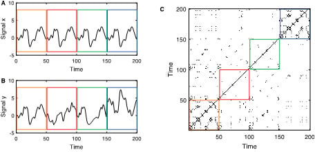
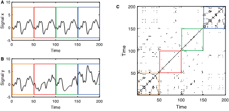
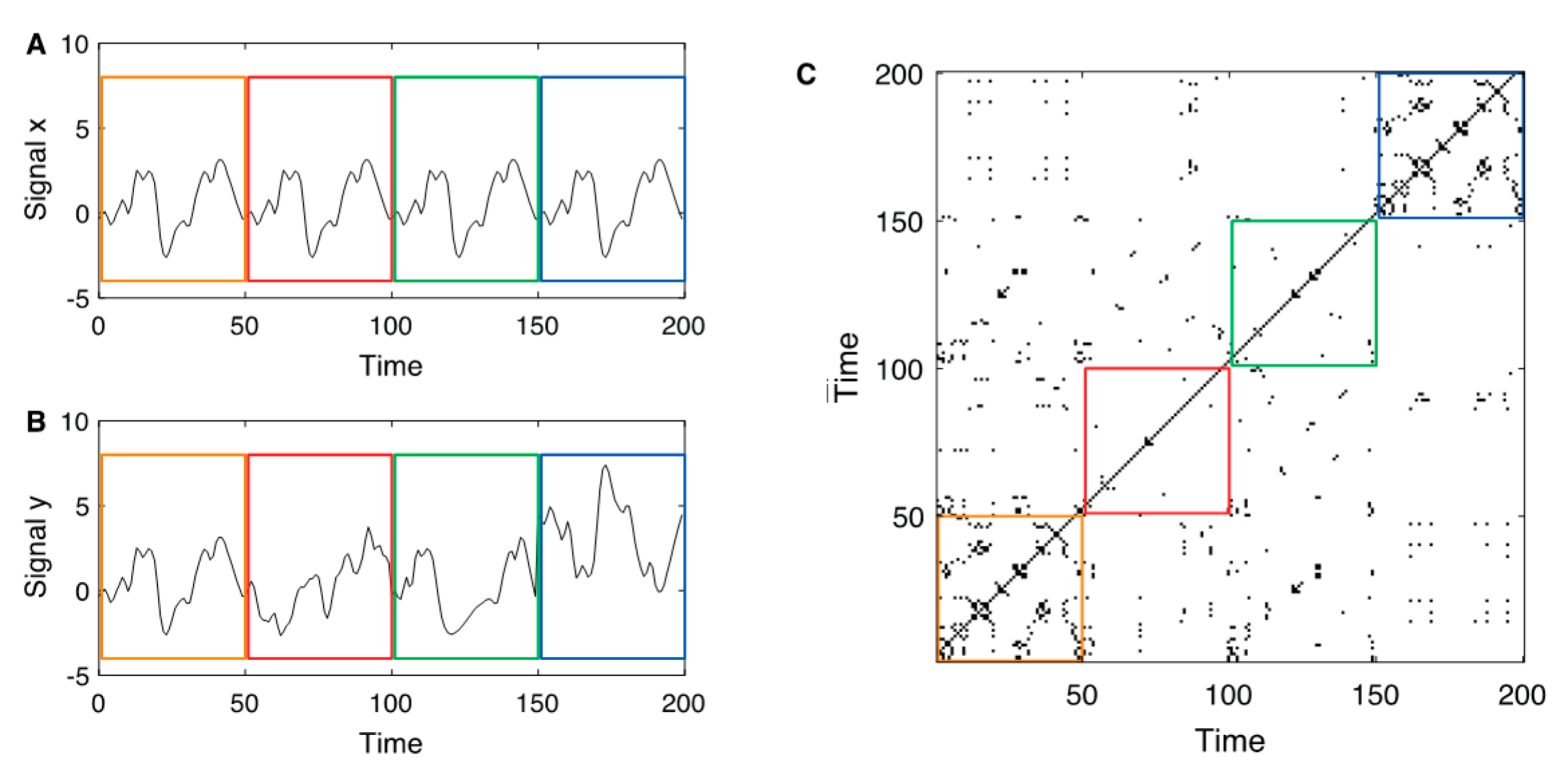
In the CRP analysis, the comparison is made between similar systems. It checks for the occurrences of similar states (values) in the analyzed signals. The main measure of similarity is the line of synchronization (LOS), which is the analogue to the main diagonal in the RP (the line of identity). If both signals are equal, the LOS is a straight line and is the main diagonal in the plot. Slight deviations in one of the systems cause a distortion of the LOS (e.g., interruptions or bendings, Figure 3c). For signals that are uncorrelated, the LOS completely vanishes. The LOS can be used to identify complete synchronization or time distortions (e.g., two periodic signals of different frequencies would have a LOS with a slope that corresponds to the ratio of the frequencies) [67]. In contrast, the JRP always has a main diagonal, because it is based on the individual RPs of each signal. Here, the comparison was performed by calculating the loss of recurrence points in the JRP relative to the individual RPs. If the considered signals share the identical recurrence patterns, the JRP is the same as the individual RPs (i.e., all recurrence points in the original RPs are preserved in the JRP). The recurrence patterns can even be the same when the signals differ at a first glance (e.g., in the first two moments). This allows for checking for generalized synchronization. In Figure 1 shows an illustration of the cross and joint recurrence plots.

In order to check for complete and generalized synchronization between the EVI, NDWI, and LST time series, we calculated the CRP and JRP between them and quantified them using the following measures. As the thresholds ${\epsilon }_x$ and ${\epsilon }_y$ were chosen to preserve the same time of the RPs for signals $x$ and $y$, the recurrence rate (RR) for both signals were identical.

For the identification and quantification of complete synchronization, we used the F-recurrence measure given by $\frac{1}{N}{\displaystyle \sum }_i{C}_{i,i}$, which quantifies the density of points along the main diagonal. The F-recurrence parameter is 1 for complete synchronization and tends to 0 for completely desynchronized systems.

This CRP and JRP analyses were combined with a sliding window approach in order to investigate the temporal change of the synchronization. We applied overlapping, sliding temporal windows with a one-year length to the original time series to calculate the F-recurrence measure before the El Niño event (from 2012 to 2014) and after (from 2016 to 2018); and before the two AMO events (for the first event from 2002 to 2004, for the second event from 2007 to 2009) and after (from 2006 to 2008 and from 2011 to 2013, respectively). For the recurrence threshold, we used an empirically defined threshold that ensured a fixed $\mathrm{RR}=0.2$. The selected value does not qualitatively affect the recurrence quantification analysis (RQA) measures [61,62,67]. The CRP and JRP analyses were carried out in MATLAB using the CRP Toolbox available at http://tocsy.pik-potsdam.de/CRPtoolbox/.

Next, we employed the Fisher test to evaluate the Gaussian distribution of the F-recurrence parameter values as well as the Student’s T-test to assess if the means of the F-recurrence parameter distributions before and after the ENSO and AMO events were the same.

4. Results

4.1. Time Series

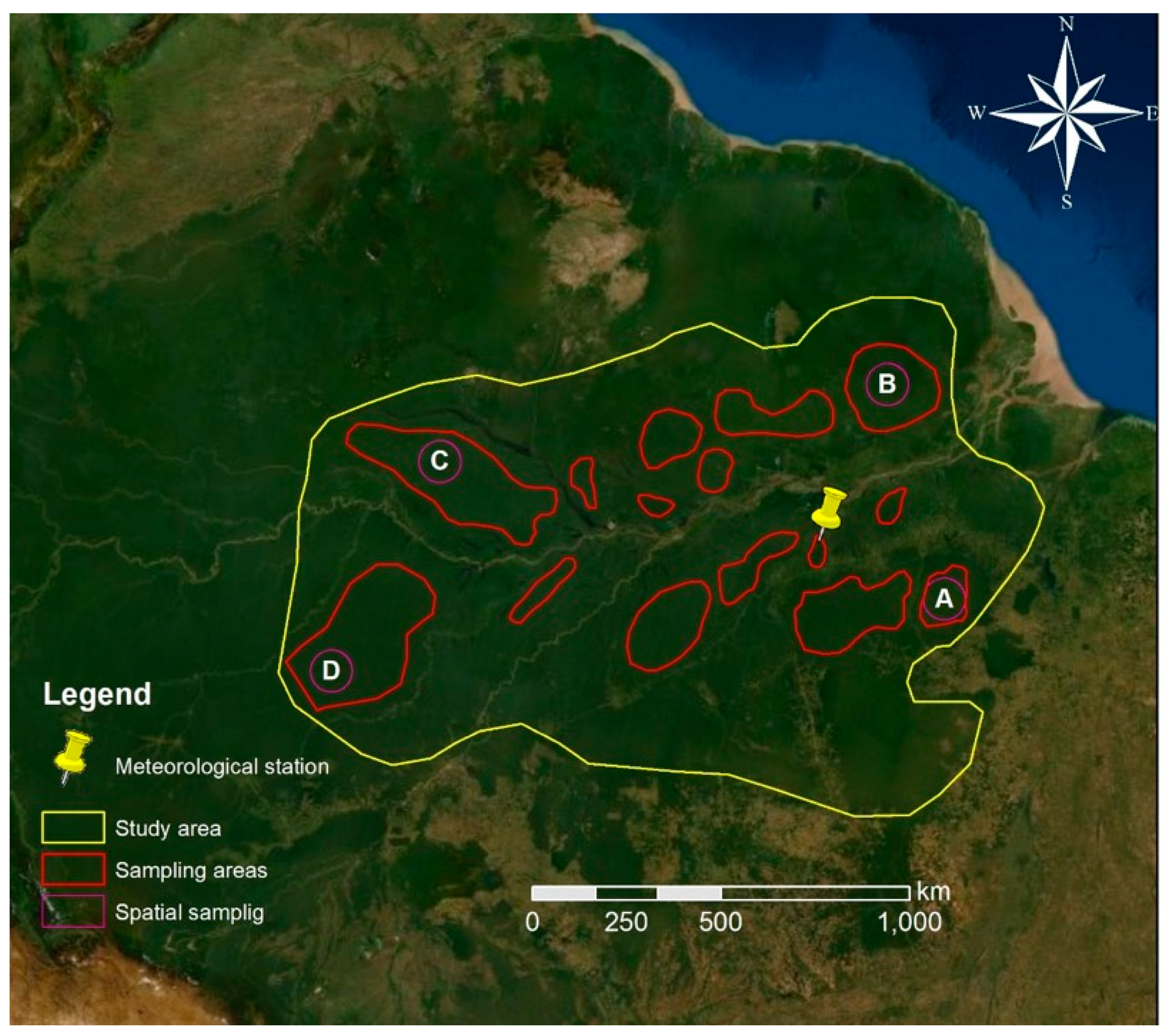
Figure 2 shows the areas of the Amazon forest selected for the present analysis. These areas showed similar spatial patterns with no changes in structure and composition during the time of the analysis (i.e., from 2001 to 2018). We can therefore rule out that changes in these areas were caused by human activities or fires. The main variation in the vegetation indices can thus be linked to the change in the ecological function of the vegetation forest due to the drought effect.

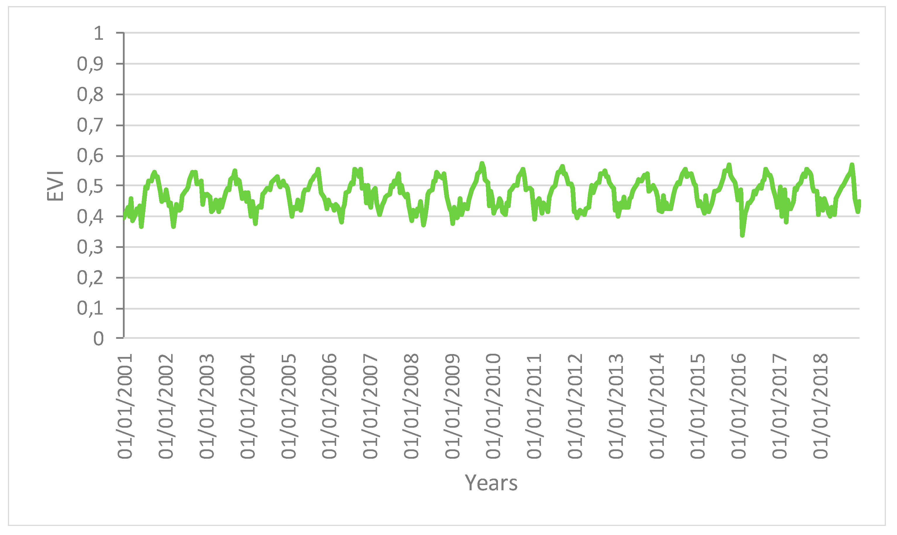
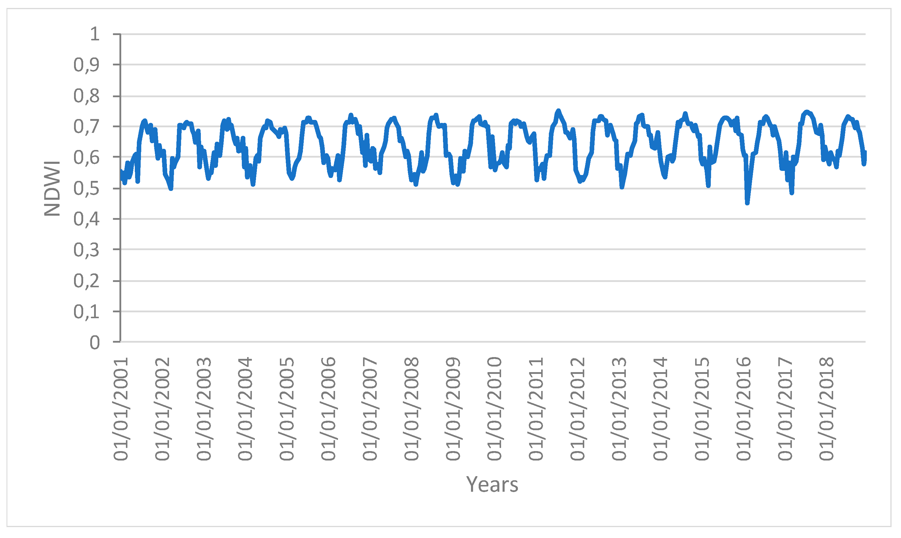
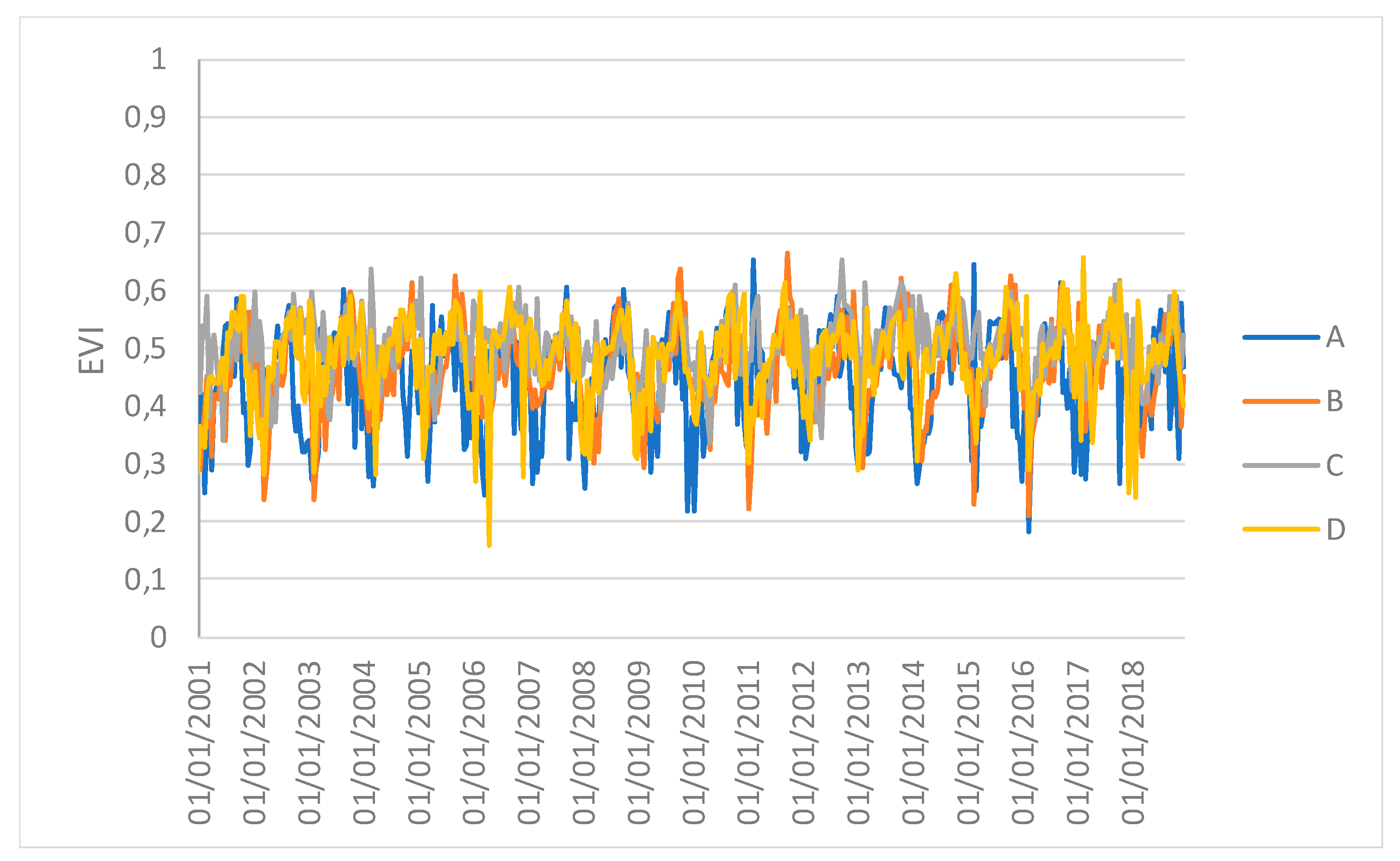
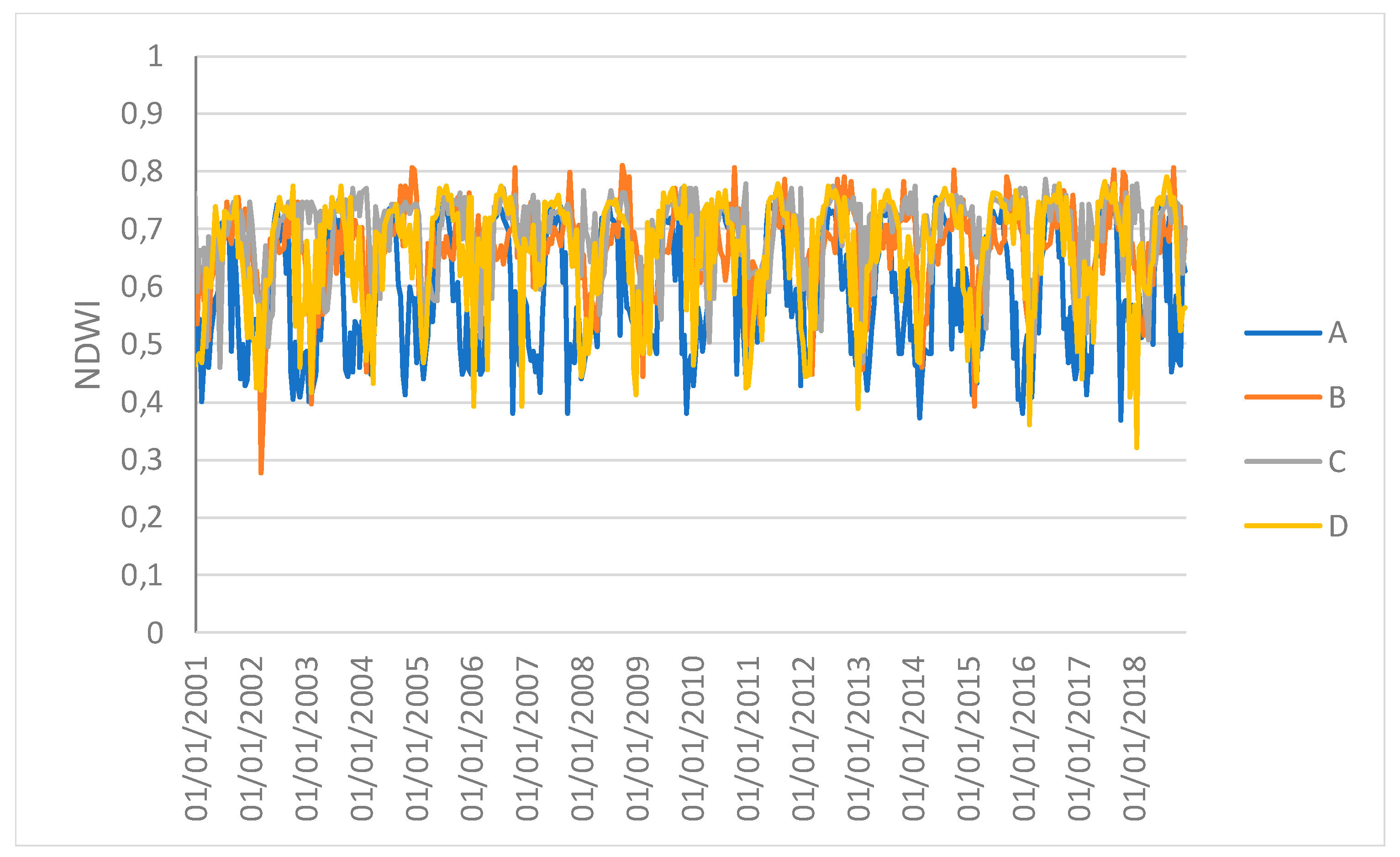
Figure 3, Figure 4 and Figure 5 show the time series profiles of the EVI, NDWI, and LST from January 2001 to December 2018 (with a frequency of 16 days) averaged over the sampling areas, whereas Figure 6 and Figure 7 show the time series of the EVI and NDWI of single sampling areas.

The profiles give an indication of the temporal variation of forest functions linked with photosynthesis in the analyzed area of the Amazon forest. The figures show that the EVI, NDWI, and LST are characterized by both periodic (represented by the wave recurrent pattern) and non-periodic (represented by peaks characterizing each wave) components.

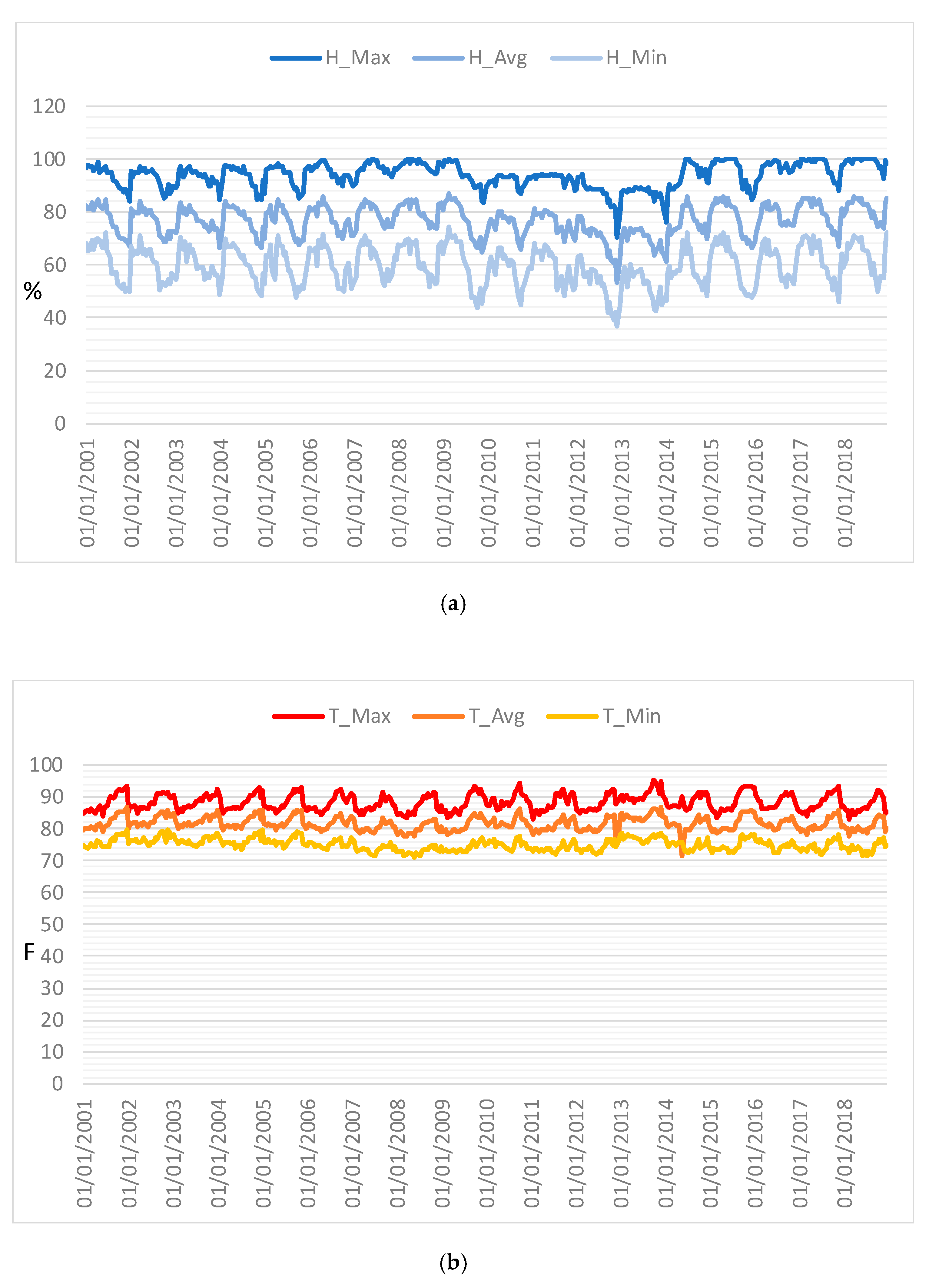
Time series of maximum temperature and humidity were also constructed from 2001 to 2018 with 16 day frequencies (Figure 8) in order to analyze the link between the ecological function of the forest and climate conditions. These profiles help to explore the specific meteorological data measured at the station of the investigated area and provide a way of assessing the meteorological variation in the area. As found for the indices, these time series were characterized by both periodic and non-periodic components.

4.2. Synchronization and Evolution Analysis

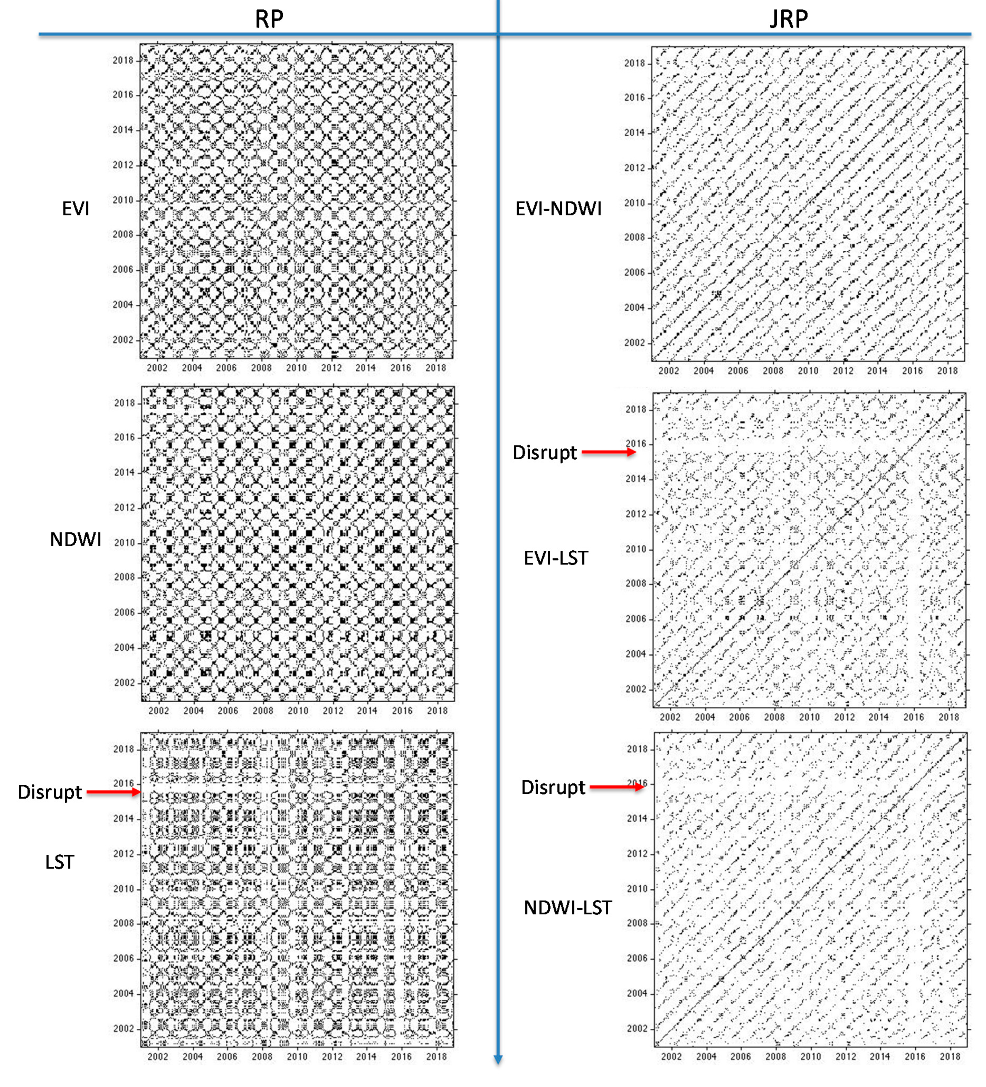
The individual RPs of the EVI and NDWI showed periodic activities representing the seasonal cycle of the forest ecosystem. The JRP between the EVI and NDWI remained as the periodic recurrence pattern over the years, with a regular and periodic temporal profile without particular variations or disruptions. This confirms the simultaneous recurrent pattern of the vegetation dynamics and photosynthetic activity within the undisturbed area (Figure 9).

In contrast, the RP of the LST revealed a disruptive event in 2015. Subsequently, the JRP showed periodic recurrences between the EVI and LST over the years, but with disruptions in the years 2015–2016 (Figure 10). The same situation was present in the JRP between the NDWI and LST. This means that some disturbing event such as an extreme climate event was causing temporal sudden changes in the system that characterizes the LST. In the last period (from 2016 to 2018), the JRP looked very similar to the individual recurrence plots of the first period (from 2001 to 2014) (i.e., the recurrence structure of both signals was the same). Therefore, the system therefore recovered its status afterward, showing a good resilience as the JRP plot maintained a similar structure after the disruption.

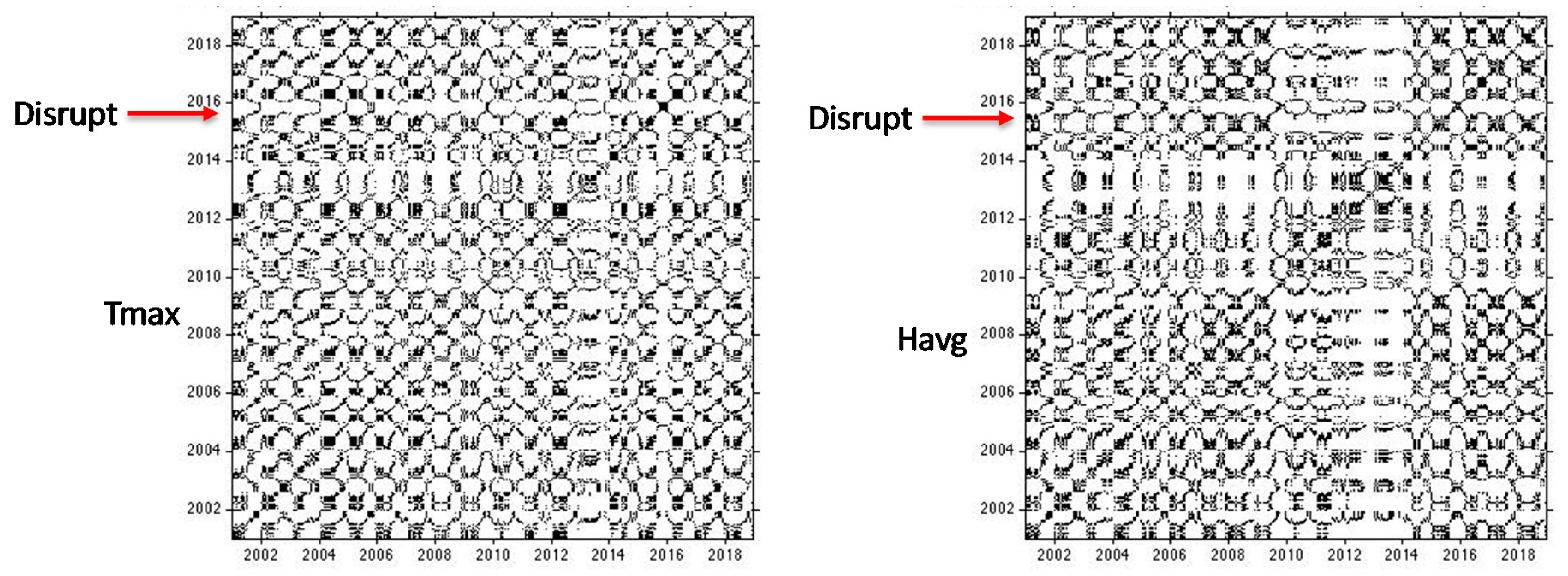
These disruptions can be linked to factors that act on short time scales [65]. By analyzing the recurrent pattern of the time series of T_max and H_avg obtained from the meteorological station, the same disruption could be observed in the same period (Figure 10). Although these meteorological data are not representative of the entire study area, they may provide greater certainty that the anomaly recorded in the LST for 2015 and 2016 was not stochastic or related to issues in the construction of the time series with MODIS images, but to a specific meteorological event. This anomaly was caused by meteorological anomalies in the short term. In particular, these disruptions observed in the RP of LST and JRP of LST and EVI/NDWI were mainly linked to the El Niño event that had a strong impact on the Amazonia in 2015 [35,51]. From the analysis of the RP of T_max and H_avg, other alterations can be noted from 2010 to 2014, which are not highlighted in the LST and even less so in the EVI and NDWI analysis. Since a single meteorological station was considered, this alteration was linked to local variations that cannot refer to the entire system.

To better identify the effect of drought events on the ecosystem function, we carried out the analysis using one-year sliding temporal windows on CRP, considering three years before and three years after 2005–2010 (AMO events) and 2015 (ENSO event). For each time window, we calculated the F-recurrence parameter for the couples EVI-NDWI, EVI-LST, and NDWI-LST. The F-recurrence varied between low and intermediate values, indicating low to intermediate synchronizations. Although the analysis explains why the values were relatively low, there were no statistically significant differences in the distribution of the F-recurrence between the period before and after the ENSO event. The p-values of the Student’s T-test were always 5% higher than the threshold (

Table 1. Statistical tests on the F-recurrence distribution calculated using sliding temporal windows of a one year length before and after the Atlantic Multidecadal Oscillation (AMO) event (year 2005).

F-Recurrence Parameter	Sample	Min.	Max.	Mean	Std. dev.	Fisher p Value	Student’s T-Test p Value	Alpha
EVI-NDWI	before	0.036	0.449	0.211	0.116	0.686	0.645	0.05
	after	0.034	0.479	0.200	0.109
EVI-LST	before	0.060	0.511	0.204	0.099	0.880	0.734
	after	0.054	0.485	0.211	0.101
NDWI-LST	before	0.038	0.477	0.205	0.113	0.669	0.846
	after	0.038	0.455	0.200	0.106

) and, thus, we cannot reject the null hypothesis that the mean values of the F-recurrence distributions before and after the drought event are similar.

This suggests that the droughts did not produce a change in the synchronization of the pattern of the variables investigated (Table 1,

Table 2. Statistical tests on the F-recurrence distribution calculated using sliding temporal windows of one year length before and after the AMO event (year 2010).

F-Recurrence Parameter	Sample	Min.	Max.	Mean	Std. dev.	Fisher p value	Student’s T-Test p value	Alpha
EVI-NDWI	before	0.051	0.565	0.204	0.119	0.679	0.948	0.05
	after	0.036	0.485	0.205	0.126
EVI-LST	before	0.054	0.529	0.208	0.114	0.719	0.949
	after	0.034	0.500	0.206	0.108
NDWI-LST	before	0.038	0.422	0.202	0.105	0.230	0.761
	after	0.018	0.477	0.209	0.125

and

Table 3. Statistical tests on the F-recurrence distribution calculated using sliding temporal windows of one year length before and after the El Niño event (year 2015).

F-Recurrence Parameter	Sample	Min.	Max.	Mean	Std. dev.	Fisher p Value	Student’s T-Test p Value	Alpha
EVI-NDWI	before	0.033	0.462	0.202	0.131	0.723	0.938	0.05
	after	0.034	0.493	0.204	0.125
EVI-LST	before	0.035	0.478	0.220	0.101	0.684	0.267
	after	0.018	0.394	0.198	0.095
NDWI-LST	before	0.033	0.538	0.220	0.116	0.542	0.249
	after	0.000	0.415	0.193	0.106

).

The F analysis for the EVI and NDWI indices was also performed for the four single sampling areas (located in different spatial locations) to verify the presence of a spatial different pattern caused by drought disturbance events. This analysis suggests that ENSO droughts events produced a change in the synchronization of the pattern of the investigated variables only for the area and the AMO events did not produce any effect (

Table 4. Statistical tests on the F-recurrence distribution calculated using sliding temporal windows of one year length before and after the AMO (2005 and 2010) and ENSO (2015) events for the single sampling areas.

Areas	F-Time	Sample	Minimum	Maximum	Mean	Std. Deviation	F p-Value	T p-Value	Alpha
A	2005	before	0.082	0.420	0.199	0.089	0.662	0.827	0.05
		after	0.035	0.493	0.195	0.095
	2010	before	0.051	0.493	0.210	0.112	0.480	0.680
		after	0.058	0.420	0.201	0.083
	2015	before	0.051	0.478	0.191	0.095	0.697	0.782
		after	0.071	0.580	0.197	0.090
B	2005	before	0.107	0.377	0.204	0.071	0.143	0.599
		after	0.038	0.413	0.213	0.088
	2010	before	0.067	0.413	0.193	0.086	0.294	0.304
		after	0.068	0.413	0.213	0.100
	2015	before	0.038	0.391	0.199	0.086	0.616	0.861
		after	0.033	0.420	0.202	0.093
C	2005	before	0.038	0.309	0.197	0.061	0.949	0.186
		after	0.118	0.377	0.211	0.045
	2010	before	0.098	0.338	0.198	0.060	0.429	0.464
		after	0.073	0.369	0.207	0.067
	2015	before	0.117	0.333	0.214	0.053	0.871	0.045
		after	0.082	0.319	0.191	0.055
D	2005	before	0.034	0.394	0.203	0.076	0.732	0.947
		after	0.060	0.394	0.202	0.080
	2010	before	0.478	0.200	0.085	0.114	0.095	0.672
		after	0.362	0.206	0.066	0.108
	2015	before	0.058	0.406	0.202	0.078	0.131	0.724
		after	0.092	0.383	0.207	0.062

).

5. Discussion

Several studies have reported on the impacts of earlier extreme temperatures and drought events on rainforests. With decreasing precipitation caused by drought events, the persistence of the structure and functions of the forest can decrease and shift to an alternative low tree-cover or low capacity to be a carbon sink [68]. However, the impacts of climate anomalies on ecosystem functions are still uncertain. Despite progress in recent years, the complex and non-linear vegetation–rainfall interactions are still poorly represented in process-based vegetation–climate studies [23,67,69].

The results obtained in this paper show that the methodology employed based on RQA is capable of assessing the resilience of a natural system to a specific disturbance event. In fact, it highlighted how the forest responded to a disturbing action due to drought events (global climate effect), which did not alter the functionality of the forest.

Specifically, the first part of the analysis showed the capacity of the area of the Amazon forest analyzed to maintain the same vegetation structure since the vegetation cover did not change at the large scale. At a smaller scale, this does not mean that drought events did not lead to the death of individual trees, because this is the main consequence of severe drought events [20,23,25,26,27].

The analysis of the synchronization of several vegetation indices that are connected to photosynthesis represents a signature that characterizes a specific ecosystem. Variations in this signature imply variations in the system. Analyzing the functions of the forest with a recurrence analysis and considering the forest as a whole, the synchronization of the vegetation indices has shown that they were not altered by drought events. An alternative explanation is that the intensity of the extreme climate events was not sufficiently strong to produce changes in the recurrence pattern of the photosynthetically active green leaf canopy and water content.

Our study therefore suggests the good adaptation of the forest to seasonal drought at the ecosystem scale. This may be linked to the capacity of the roots to use the deep soil water, maintaining the water tension in the xylem relatively constant in both wet or dry seasons [70,71,72]. A combination of access to deep soil water, which helps to ensure evergreen canopies during dry seasons, and the low cloudiness during the dry season, helps the photosynthesis to continue [24]. This may also be linked to the higher quantity of light available for the forest during dry events, which is more limiting than water for tropical forest productivity [73,74].

Warm SSTs over the tropical Pacific (ENSO) induced changes in the atmospheric circulation, which had short temporal effects on the synchronization of the vegetation indices and are different from the changes induced by warm SSTs over the tropical Atlantic. The only variation detected was relative to the LST during ENSO events. This is influenced by the atmospheric temperature, but also by the capacity of the vegetation to mitigate the microclimate with the evapotranspiration of the plants. This local temporal alteration may thus also be interpreted as a lower ability of the forest to mitigate the local microclimate due to stress. However, the disruption was not irreversible and was highlighted only during the ENSO event. Thus, it did not affect the synchronization of the vegetation indices before and after the event.

Considering the similar structure of the vegetation forest, this suggests that the functionality of the forest in relation to photosynthetic activity may be similar before and after the event. The high capacity of the forest to absorb the disturbance can be explained by the feedback of the drought events which, aside from leading to the deaths of individual trees, can produce a “green up” at the ecosystem level, and which increases in solar radiation during drier periods that boost tropical productivity. Therefore, this creates a new opportunity to develop an ecological function with a higher resilience [75,76,77,78,79].

However, the results obtained in this study may be affected by the selection of sampling areas. Furthermore, the 1 km spatial resolution of the images and, especially, the spatially-averaged values, which might hide local variations, can reduce the capacity of the vegetation indices to discriminate the differences. Therefore, the results can be considered valid at the ecosystem scale. Moreover, the time series of spatial averages can hide the spatial variability that the drought events can generate. Repeating the analysis F between the EVI and NDWI for single samples at four different points revealed that only sample C had a different synchronization after the ENSO. This study can thus be used to identify both a global response of the forest system and specific individual local responses.

Focusing on the potential of the RQA, this study has however demonstrated the ability of the method to highlight different recurrence patterns of the vegetation time series caused by disturbance events.

Of course, this methodology does not replace other methodologies commonly employed in the literature, however, it should be considered as an approach that offers a different view in the study of the dynamics of natural systems.

6. Conclusions

Drought events generated by AMO in 2005 and 2010 did not induce functional changes in the forest ecosystem, while the drought event occurring in 2015, linked to ENSO, produced an immediate variation in LST, which, however, did not do any irreversible damage to the functionality of the forest system. The forest thus showed a good functional resilience to the drought events that occurred in the three years.

These findings refer to the specific RQA analysis applied to the selected ecosystem proxies. Specifically, the “retrospective analysis” using RQA applied to the vegetation indices enabled us to understand the past trajectory of a portion of the Amazon forest. The RQA highlighted the recurrent pattern of the natural processes linked to disturbance events in the short and medium term as well as the system response and its ability to recover.

In the first part of the analysis, the RQA evaluated the effect of the climatic disturbances on the evolution of the vegetation indices, that is, at the ecosystem level, the forest was able to overcome the extreme event of ENSO observed in 2015. Under continued global warming and a projected increase in the frequency of ENSO events, more frequent record-breaking climate extremes are expected in Amazonia [80]. We are thus confident that the approach followed here will be useful to evaluate the direct effects of these extreme events on the evolution of the capacity of the forest to maintain its ecological functions.

This approach could also be useful to understand the evolution of the system and its response after the fire that affected a large area of the forest in 2019. A change in the forest functions due to selective logging or below canopy burning, which are not easily detectable from greenness changes, could also be revealed using the RQA. This is important, because although of anthropogenic origin, fires in forested areas have been suggested as having the biggest impact on forest transition under an increased drought frequency scenario [63,81].

Overall, this work has highlighted the following potential of the RQA:

• it provides an immediate and simple interpretation of the results through plot visualization;
• it can be applied to short time series and allows an objective interpretation of specific variations;
• it evaluates the ecological resilience, which relates to the magnitude of the disturbance that a system can absorb before shifting to another ecological condition [81]; and
• it highlights the panarchy of processes at different spatial and temporal scales (e.g., the effect of the large scale ENSO on the smaller scale Amazon system).

Future developments could involve, for example, (i) extending the research to the entire Amazon forest to understand if the findings are representative of the whole biome; (ii) calibrations through field measurements that would improve the analysis; and (iii) the direct comparison of CO₂ emissions to better understand the feedback between human activities, climate conditions, and photosynthesis activity.

The vegetation indices approach clearly provides general information on the dynamics linked to the functions of the forest at the large scale, however, it cannot provide specific indications in relation to the small changes to individual plants caused by extreme events. Our analysis should therefore be integrated with local scale samplings.

References

- Janzen, H.H. Carbon cycling in earth systems—A soil science perspective. Agric. Ecosyst. Environ. 2004, 104, 399–417. [Google Scholar] [CrossRef]
- Espirito-Santo, F.; Gloor, M.; KelleriD, M.; Malhi, Y.; Saatchi, S.; Nelson, B.; Junior, R.C.O.; Pereira, C.; Lloyd, J.; Frolking, S.; et al. Size and frequency of natural forest disturbances and the Amazon forest carbon balance. Nat. Commun. 2014, 5, 3434. [Google Scholar] [CrossRef] [PubMed]
- Qie, L.; Lewis, S.L.; Sullivan, M.J.P.; Lopez-Gonzalez, G.; Pickavance, G.C.; Sunderland, T.; Ashton, P.; Hubau, W.; Abu Salim, K.; Aiba, S.-I.; et al. Long-term carbon sink in Borneo’s forests halted by drought and vulnerable to edge effects. Nat. Commun. 2017, 8, 1966. [Google Scholar] [CrossRef] [PubMed]
- Keeling, C.D.; Chin, J.F.S.; Whorf, T.P. Increased activity of northern vegetation inferred from atmospheric CO2 measurements. Nature 1996, 382, 146–149. [Google Scholar] [CrossRef]
- Myneni, R.B.; Keeling, C.D.; Tucker, C.J.; Asrar, G.; Nemani, R.R. Increased plant growth in the northern high latitudes from 1981 to 1991. Nature 1997, 386, 698–702. [Google Scholar] [CrossRef]
- Houghton, R.A. Keeping management effects separate from environmental effects in terrestrial carbon accounting. Glob. Chang. Biol. 2013, 19, 2609–2612. [Google Scholar] [CrossRef] [PubMed]
- Goetz, S.J.; Bunn, A.G.; Fiske, G.J.; Houghton, R.A. Satellite-observed photosynthetic trends across boreal North America associated with climate and fire disturbance. PNAS 2005, 102, 13521–13525. [Google Scholar] [CrossRef]
- Liu, J.; Chen, J.M.; Cihlar, J.; Chen, W. Net primary productivity distribution in the BOREAS region from a process model using satellite and surface data. J. Geophys. Res. 1999, 104, 27735–27754. [Google Scholar] [CrossRef]
- Odum, H.T. Environment, Power, and Society; John Wiley & Sons: Hoboken, NJ, USA, 1971; ISBN 13 978-0471652755. [Google Scholar]
- Jackson, T.J.; Chen, D.; Cosh, M.; Li, F.; Anderson, M.; Walthall, C.; Doriaswamy, P.; Hunt, E.R. Vegetation water content mapping using Landsat data derived normalized difference water index for corn and soybeans. Remote Sens. Environ. 2004, 92, 475–482. [Google Scholar] [CrossRef]
- MEA, Millennium Ecosystem Assessment. Ecosystems and Human WellBeing: Current State and Trends; Island Press: Washington, DC, USA, 2005; ISBN 9781559632270. [Google Scholar]
- Costanza, R.; Fisher, B.; Mulder, K.; Liu, S.; Christopher, T. Biodiversity and ecosystem services: A multi-scale empirical study of the relationship between species richness and net primary production. Ecol. Econ. 2007, 61, 478–491. [Google Scholar] [CrossRef]
- Richmond, A.; Kaufmann, R.K.; Mynen, R.B. Valuing ecosystem services: A shadow price for net primary production. Ecol. Econ. 2007, 64, 454–462. [Google Scholar] [CrossRef]
- Bishop, J.D.K.; Amaratunga, G.A.J. Quantifying the limits of HANPP and carbon emissions with prolong total species well-being. Environ. Dev. Sustain. 2010, 12, 213–231. [Google Scholar] [CrossRef]
- Semeraro, T.; Vacchiano, G.; Aretano, R. Application of vegetation index time series to value fire effect on primary production in a Southern European rare wetland. Ecol. Eng. 2019, 134, 9–17. [Google Scholar] [CrossRef]
- Jax, K. Ecosystem Functioning; Cambridge University Press: Cambridge, UK, 2010; ISBN 9780511781216. [Google Scholar]
- Holling, C.S.; Gunderson, L.; Peterson, G. Sustainability and Panarchies. In Panarchy: Understanding Transformations in Human and Natural Systems; Gunderson, L.H., Holling, C.S., Eds.; Island Press: Washington, DC, USA, 2002; pp. 63–102. [Google Scholar]
- Xu, C.; Li, Y.; Hu, J.; Yang, X.; Sheng, S.; Liu, M. Evaluating the difference between the normalized difference vegetation index and net primary productivity as the indicators of vegetation vigor assessment at landscape scale. Environ. Monit. Assess. 2012, 184, 1275–1286. [Google Scholar] [CrossRef]
- Michelle, O.; Timothy, R.; Monteagudo, M.; Roel, J.W.; Ted, R.; Nigel, C.A.; Jose Lui, S.C.; Susan, G.W.; William, F.; Vargas, N.; et al. Hyperdominance in Amazonian forest carbon cycling. Nat. Commun. 2014, 6, 6857. [Google Scholar]
- Stark, S.C.; Leitold, V.; Wu, J.; Hunter, M.; De Castilho, C.V.; Costa, F.R.C.; McMahon, S.M.; Parker, G.G.; Shimabukuro, M.T.; Lefsky, M.; et al. Amazon forest carbon dynamics predicted by profiles of canopy leaf area and light environment. Ecol. Lett. 2012, 15, 1406–1414. [Google Scholar] [CrossRef]
- Yang, Y.; Saatchi, S.S.; Xu, L.; Yu, Y.; Choi, S.; Phillips, N.; Kennedy, R.; Keller, M.; Knyazikhin, Y.; Myneni, R.B. Post-drought decline of the Amazon carbon sink. Nat. Commun. 2018, 9, 3172. [Google Scholar] [CrossRef]
- Tyukavina, A.; Hansen, M.C.; Potapov, P.V.; Stehman, S.V.; Smith-Rodriguez, K.; Okpa, C.; Aguilar, R. Types and rates of forest disturbance in Brazilian Legal Amazon, 2000–2013. Sci. Adv. 2017, 3, e1601047. [Google Scholar] [CrossRef]
- Phillips, O.L.; Aragão, L.E.O.C.; Lewis, S.L.; Fisher, J.B.; Lloyd, J.; Lopez-Gonzalez, G.; Malhi, Y.; Monteagudo, A.; Peacock, J.; Quesada, C.A.; et al. Drought Sensitivity of the Amazon Rainforest. Science 2009, 323, 1344–1347. [Google Scholar] [CrossRef]
- Davidson, E.A.; De Araújo, A.C.; Artaxo, P.; Balch, J.K.; Brown, I.F.; Bustamante, M.; Coe, M.T.; DeFries, R.S.; KelleriD, M.; LongoiD, M.; et al. The Amazon basin in transition. Nature 2012, 481, 321–328. [Google Scholar] [CrossRef]
- Nepstad, D.C.; Tohver, I.M.; Ray, D.; Moutinho, P.; Cardinot, G. Mortality of large trees and lianas following experimental drought in an Amazon forest. Ecology 2017, 88, 2259–2269. [Google Scholar] [CrossRef] [PubMed]
- Williamson, G.B.; Laurance, W.F.; Oliveira, A.A.; Delamônica, P.; Gascon, C.; Lovejoy, T.E.; Pohl, L. Amazonian tree mortality during the 1997 El Niño drought. Conserv. Biol. 2000, 14, 1538–1542. [Google Scholar] [CrossRef]
- Hilker, T.; Lyapustin, A.I.; Tucker, C.J.; Hall, F.G.; Myneni, R.B.; Wang, Y.; Bi, J.; de Moura, Y.M.; Sellers, P.J. Vegetation dynamics and rainfall sensitivity of the Amazon. PNAS 2014, 111, 16041–16046. [Google Scholar] [CrossRef]
- Moorcroft, P.; Hurtt, G.; Pacala, S. A method for scaling vegetation dynamics: The ecosystem demography model (ED). Ecol. Monogr. 2001, 71, 557–586. [Google Scholar] [CrossRef]
- Holling, C.S. Engineering resilience versus ecological resilience Engineering Within Ecological Constraints. In Engineering within Ecological Constraints; Schulze, P.E., Ed.; National Academy Press: Washington, DC, USA, 1996; pp. 31–43. [Google Scholar]
- Gunderson, L.H.; Holling, C.S. (Eds.) Panarchy: Understanding Transformations in Systems of Humans and Nature; Island Press: Washington, DC, USA, 2002. [Google Scholar]
- IPCC. Climate Change 2014: Synthesis Report. Contribution of Working Groups I, II and III to the Fifth Assessment Report of the Intergovernmental Panel on Climate Change; Core Writing Team, Pachauri, R.K., Meyer, L.A., Eds.; IPCC: Geneva, Switzerland, 2014. [Google Scholar]
- Perz, S.G.; Muñoz-Carpena, R.; Kiker, G.; Holt, R.D. Evaluating ecological resilience with global sensitivity and uncertainty analysis. Remote Sens. Environ. 2004, 91, 256–270. [Google Scholar] [CrossRef]
- Zurlini, G.; Marwan, N.; Semeraro, T.; Jones, K.B.; Areatno, R.; Pasimeni, M.R.; Valente, D.; Mulder, C.; Petrosillo, I. Investigating landscape phase transitions in Mediterranean rangelands by recurrence analysis. Landsc. Ecol. 2018, 33, 1617–1631. [Google Scholar] [CrossRef]
- Zurlini, G.; Zaccarelli, N.; Petrosillo, I. Indicating retrospective resilience of multi-scale patterns of real habitats in a landscape. Ecol. Indic. 2006, 6, 184–204. [Google Scholar] [CrossRef]
- Barbosa, C.C.A.; Atkinson, P.M.; Dearing, J.A. Remote sensing of ecosystem services: A systematic review. Ecol. Indic. 2015, 52, 430–443. [Google Scholar] [CrossRef]
- Rouse, J.W.; Haas, R.H.; Schell, J.A.; Deering, D.W. Monitoring vegetation systems in the Great Plains with ERTS. In Proceedings of the 3rd ERTS Symposium Washington, DC, USA, 10–14 December 1973; NASA: Washington, DC, USA, 1973; Volume 1, pp. 309–317. [Google Scholar]
- Myneni, R.B.; Hall, F.G.; Sellers, P.J.; Marshak, A.L. The interpretation of spectral vegetation indexes. IEEE Geosci. Remote Sens. 1995, 33, 481–486. [Google Scholar] [CrossRef]
- Xiao, X.; Zhang, Q.; Braswell, B.; Urbanski, S.; Boles, S.; Wofsy, S.; Moore III, B.; Ojima, D. Modeling gross primary production of temperate deciduous broadleaf forest using satellite images and climate data. Remote Sens. Environ. 2004, 91, 256–270. [Google Scholar] [CrossRef]
- Zaccarelli, N.; Li, B.-L.; Petrosillo, I.; Zurlini, G. Order and disorder in ecological time series: Introducing normalized spectral entropy. Ecol. Indic. 2013, 28, 22–30. [Google Scholar] [CrossRef]
- Parrott, L. Quantifying the complexity of simulated spatiotemporal population dynamics. Ecol. Complex. 2005, 2, 175–184. [Google Scholar] [CrossRef]
- Jacquin, A.; Sheeren, D.; Lacombe, J.P. Vegetation cover degradation assessment in Madagascar savanna based on trend analysis of MODIS NDVI time series. Int. J. Appl. Earth Obs. Geoinf. 2010, 12, S3–S10. [Google Scholar] [CrossRef]
- Sabo, J.L.; Post, D.M. Quantifying periodic, stochastic, and catastrophic environmental variation. Ecol. Monogr. 2008, 78, 19–40. [Google Scholar] [CrossRef]
- Ives, A.R.; Abbott, K.C.; Ziebarth, N.L. Analysis of ecological time series with ARMA(p,q) models. Ecology 2010, 91, 858–871. [Google Scholar] [CrossRef]
- Jimenez, J.C.; Libonati, R.; Peres, L.F. Droughts Over Amazonia in 2005, 2010, and 2015: A Cloud Cover Perspective. Front. Earth Sci. 2018, 6, 227. [Google Scholar] [CrossRef]
- Jiménez-Muñoz, J.C.; Mattar, C.; Barichivich, J.; Santamaría-Artigas, A.; Takahashi, K.; Malhi, Y.; Sobrino, J.A.; Schrier, G.V. Record-breaking warming and extreme drought in the Amazon rainforest during the course of El Niño 2015–2016. Sci. Rep. 2019, 6, 33130. [Google Scholar] [CrossRef]
- Coelho, C.A.S.; Cavalcanti, I.A.F.; Costa, S.; Freitas, S.R.; Ito, E.R.; Luz, G.; Santos, A.F.; Nobre, C.A.; Marengo, J.A.; Pezza, A.B. Climate diagnostics of three major drought events in the Amazon and illustrations of their seasonal precipitation predictions. Meteorol. Appl. 2012, 19, 237–255. [Google Scholar] [CrossRef]
- Marengo, J.A.; Nobre, C.A.; Tomasella, J.; Cardosa, M.F.; Oyama, M.D. Hydro-climate and ecological behaviour of the drought of Amazonia in 2005. Philos. Trans. R. Soc. B 2008, 363, 1773–1778. [Google Scholar] [CrossRef]
- MODIS Images. Available online: https://lpdaac.usgs.gov/dataset_discovery/modis/modis_products_table (accessed on 12 November 2019).
- Boles, S.; Xiao, X.; Liu, J.; Zhang, Q.; Munkhutya, S.; Chen, S.; Ojima, D. Land cover characterization of Temperate East Asia: Using multi-temporal image data of VEGETATION sensor. Remote Sens. Environ. 2004, 90, 477–489. [Google Scholar] [CrossRef]
- Xiao, X.; Hollinger, D.; Aber, J.D.; Goltz, M.; Davidson, E.A.; Zhang, Q.Y. Satellite-based modeling of gross primary production in an evergreen needle leaf forest. Remote Sens. Environ. 2004, 89, 519–534. [Google Scholar] [CrossRef]
- Zhang, X.Y.; Friedl, M.A.; Schaaf, C.B.; Strahler, A.H.; Hodges, J.C.F.; Gao, F.; Reed, B.C.; Huete, A. Monitoring vegetation phenology using MODIS. Remote Sens. Environ. 2003, 84, 471–475. [Google Scholar] [CrossRef]
- Xiao, X.; Braswell, B.; Zhang, Q.; Boles, S.; Frolking, S.; Moore, B. Sensitivity of vegetation indices to atmospheric aerosols: Continental-scale observations. Remote Sens. Environ. 2003, 84, 385–392. [Google Scholar] [CrossRef]
- Ceccato, P.; Flasse, S.; Tarantola, S.; Jacquemond, S.; Gregoire, J.M. Detecting vegetation water content using reflectance in the optical domain. Remote Sens. Environ. 2001, 77, 22–33. [Google Scholar] [CrossRef]
- Ceccato, P.; Gobron, N.; Flasse, S.; Pinty, B.; Tarantol, S. Designing a spectral index to estimate vegetation water content from remote sensing data: Part 1: Theoretical approach. Remote Sens. Environ. 2002, 82, 188–197. [Google Scholar] [CrossRef]
- Hopkins, W.G.; Hüner, N.P.A. Introduction to Plant Physiology; John Wiley & Sons, Inc.: Hoboken, NJ, USA, 2004. [Google Scholar]
- Gu, Y.; Brown, J.F.; Verdin, J.P.; Wardlow, B. A five-year analysis of MODIS NDVI and NDWI for grassland drought assessment over the central Great Plains of the United States. Geophys. Res. Lett. 2007, 34, L06407. [Google Scholar] [CrossRef]
- Gu, Y.; Hunt, E.; Wardlow, B.; Basara, J.B.; Brown, J.F.; Verdin, J.P. Evaluation of MODIS NDVI and NDWI for vegetation drought monitoring using Oklahoma Mesonet soil moisture data. Geophys. Res. Lett. 2008, 35, L22401. [Google Scholar] [CrossRef]
- Ceccato, P.; Flasse, S.; Gregoire, J.M. Designing a spectral index to estimate vegetation water content from remote sensing data: Part 2. Validation and applications. Remote Sens. Environ. 2002, 82, 198–207. [Google Scholar] [CrossRef]
- Gao, B.C. NDWI—A normalized difference water index for remote sensing of vegetation liquid water from space. Remote Sens. Environ. 1996, 58, 257–266. [Google Scholar] [CrossRef]
- Lillesand, T.M.; Kiefer, R.M. Remote Sensing and Image Interpretation, 4th ed.; John Wiley & Sons, Inc.: Hoboken, NJ, USA, 2000. [Google Scholar]
- Weather Underground. Available online: https://www.wunderground.com/weather/br/santar%C3%A9m/-2.44,-54.70 (accessed on 12 November 2019).
- Marwan, N.; Kurths, J.; Foerster, S. Analysing spatially extended high-dimensional dynamics by recurrence plots. Phys. Lett. A 2015, 379, 894–900. [Google Scholar] [CrossRef]
- Semeraro, T.; Marwan, N.; Jones, B.; Aretano, R.; Pasimeni, M.R.; Petrosillo, I.; Mulder, C.; Zurlini, G. Recurrence analysis of vegetation time series and phase transitions in Mediterranean rangelands. arXiv 2017, arXiv:1705.04813. [Google Scholar]
- Zurlini, G.; Petrosillo, I.; Aretano, R.; Castorini, I.; D’Arpa, S.; De Marco, A.; Pasimeni, M.R.; Semeraro, T.; Zaccarelli, N. Key fundamental aspects for mapping and assessing ecosystem services: Predictability of ecosystem service providers at scales from local to global. Ann. Di Bot. 2014, 4, 53–63. [Google Scholar]
- Romano, M.; Thiel, M.; Kurths, J.; Von Bloh, W. Multivariate recurrence plots. Phys. Lett. A 2004, 330, 214–223. [Google Scholar] [CrossRef]
- Marwan, N.; Carmen Romano, M.; Thiel, M.; Kurths, J. Recurrence plots for the analysis of complex systems. Phys. Rep. 2007, 438, 237–329. [Google Scholar] [CrossRef]
- Marwan, N.; Thiel, M.; Nowaczyk, N.R. Cross Recurrence Plot Based Synchronization of Time Series. Nonlinear Process. Geophys. 2002, 9, 325–331. [Google Scholar] [CrossRef]
- Bonal, D.; Bosc, A.; Goret, J.Y.; Burban, B.; Gross, P.; Bonnefond, J.M.; Elbers, J.; Ponton, S.; Epron, D.; Guehl, J.M.; et al. The impact of severe dry season on net ecosystem exchange in the Neotropical rainforest of French Guiana. Glob. Chang. Biol. 2008, 14, 1917–1933. [Google Scholar] [CrossRef]
- Delphine, C.Z. Self-amplified Amazon forest loss due to vegetation-atmosphere feedbacks. Nat. Commun. 2017, 8, 14681. [Google Scholar]
- Scheffer, M.; Holmgren, M.; Brovkin, V.; Claussen, M. Synergy between small-and large-scale feedbacks of vegetation on the water cycle. Glob. Chang. Biol. 2005, 11, 1003–1012. [Google Scholar] [CrossRef]
- van Nes, E.H.; Hirota, M.; Holmgren, M.; Scheffer, M. Tipping points in tropical tree cover: Linking theory to data. Glob. Chang. Biol. 2014, 20, 1016–1021. [Google Scholar] [CrossRef]
- Fisher, R.A.; Williams, M.; Lobo do Vale, R.; Costa, A.; Meir, P. Evidence from Amazonian forests is consistent with isohydric control of leaf water potential. PlantCell Environ. 2006, 29, 151–165. [Google Scholar] [CrossRef]
- Brando, P.M.; Nepstad, D.C.; Davidson, E.A.; Trumbore, S.E.; Ray, D.; Camargo, P. Drought effects on litterfall, wood production, and belowground carbon cycling in an Amazon forest: Results of a throughfall reduction experiment. Philos. Trans. R. Soc. B 2008, 363, 1839–1848. [Google Scholar] [CrossRef] [PubMed]
- Da Costa, A.C.L.; Galbraith, D.; Almeida, S.; Portela, B.T.T.; Da Costa, M.; Junior, J.D.A.S.; Braga, A.P.; De Gonçalves, P.H.L.; De Oliveira, A.A.; Fisher, R.A.; et al. Effect of 7 yr of experimental drought on vegetation dynamics and biomass storage of an eastern Amazonian rainforest. New Phytol. 2010, 187, 579–591. [Google Scholar] [CrossRef]
- Morton, D.C.; Nagol, J.; Carabajal, C.C.; Rosette, J.; Palace, M.; Cook, B.D.; Vermote, E.F.; Harding, D.J.; North, P.R.J. Amazon forests maintain consistent canopy structure and greenness during the dry season. Nature 2014, 506, 221–224. [Google Scholar] [CrossRef] [PubMed]
- Saleska, S.R.; Miller, S.D.; Matross, D.M.; Goulden, M.; Wofsy, S.C.; Da Rocha, H.R.; De Camargo, P.B.; Crill, P.M.; Daube, B.C.; De Freitas, H.C.; et al. Carbon in Amazon forests: Unexpected seasonal fluxes and disturbance-induced losses. Science 2003, 302, 1554–1557. [Google Scholar] [CrossRef]
- Huete, A.; Didan, K.; Shimabukuro, Y.E.; Ratana, P.; Saleska, S.R.; Yang, W.; Hutyra, L.R.; Nemani, R.; Myneni, R. Amazon rainforests green-up with sunlight in dry season. Geophys. Res. Lett. 2006, 13, L06405. [Google Scholar] [CrossRef]
- Saleska, S.R.; Didan, K.; Huete, A.R.; da Rocha, H.R. Amazon Forests Green-Up During 2005 Drought. Science 2007, 318, 612. [Google Scholar] [CrossRef]
- Condit, R.; Aguilar, S.; Hernandez, A.; Perez, R.; Lao, S.; Angehr, G.; Hubbell, S.P.; Foster, R.B. Tropical forest dynamics across a rainfall gradient and the impact of an El Niño dry season. J. Trop. Ecol. 2004, 20, 51–72. [Google Scholar] [CrossRef]
- Graham, E.A.; Mulkey, S.; Kitajima, K.; Phillips, K.N.; Wright, S.J. Cloud cover limits net CO2 uptake and growth of a rainforest tree during tropical rainy seasons. PNAS 2013, 100, 572–576. [Google Scholar] [CrossRef]
- Aragão, L.E.O.C.; Malhi, Y.; Roman-Cuesta, R.M.; Saatchi, S.; Anderson, L.O.; Shimabukuro, Y.E. Spatial patterns and fire response of recent Amazonian droughts. Geophys. Res. Lett. 2007, 34, L07701. [Google Scholar] [CrossRef]
Figure 1.
(A) Exemplary reference signal with a pattern that repeats four times (separated by the coloured boxes); (B) exemplary second signal with identical pattern as the reference signal in the first epoch, a completely different, uncorrelated signal in the second epoch, identical signal as the reference but time-deformed in the third epoch (where the time axis is distorted by the function , and a transformed reference signal in the last epoch. (C) Joint recurrence plot between the two signals and . As the main diagonal is present in the individual recurrence plots, it is also present in the joint recurrence plot. The first epoch with the identical segments corresponds to the individual recurrence plots (which are identical for and ). During the second and third epochs, the recurrence structure of and differ, therefore, the JRPs are almost empty during these epochs. In the last epoch, the sub-JRP looks very similar to the individual recurrence plots (akin the sub-JRP in the first box): the recurrence structure of both signals is equal, although the state values differ.
Figure 2.
Study area (yellow) and sampling areas (red) where the time series of the enhanced vegetation index (EVI), normalized difference water index (NDWI) and land surface temperature (LST) were extracted, with indication of further spatial sampling (purple) areas subjected to local analysis of the same time series (modified from Bing Maps).
Figure 3.
Time series profiles of the EVI for the area not affected by human disturbance.
Figure 4.
Time series profiles of the NDWI area not affected by human disturbance.
Figure 5.
Time series profiles of the LST.
Figure 6.
Time series profiles of the EVI of single sampling areas.
Figure 7.
Time series profiles of the NDWI of single sampling areas.
Figure 8.
Time series profiles of (a) humidity and (b) temperature.
Figure 9.
RP of the Tmax and Havg time series.
Figure 10.
Recurrence plot (RP) and joint recurrent plot (JRP) of the EVI, NDWI and LST time series.