Abstract
The thermal-based two-source energy balance (TSEB) model has accurately simulated energy fluxes in a wide range of landscapes with both remote and proximal sensing data. However, tree-grass ecosystems (TGE) have notably complex heterogeneous vegetation mixtures and dynamic phenological characteristics presenting clear challenges to earth observation and modeling methods. Particularly, the TSEB modeling structure assumes a single vegetation source, making it difficult to represent the multiple vegetation layers present in TGEs (i.e., trees and grasses) which have different phenological and structural characteristics. This study evaluates the implementation of TSEB in a TGE located in central Spain and proposes a new strategy to consider the spatial and temporal complexities observed. This was based on sensitivity analyses (SA) conducted on both primary remote sensing inputs (local SA) and model parameters (global SA). The model was subsequently modified considering phenological dynamics in semi-arid TGEs and assuming a dominant vegetation structure and cover (i.e., either grassland or broadleaved trees) for different seasons (TSEB-2S). The adaptation was compared against the default model and evaluated against eddy covariance (EC) flux measurements and lysimeters over the experimental site. TSEB-2S vastly improved over the default TSEB performance decreasing the mean bias and root-mean-square-deviation (RMSD) of latent heat (LE) from 40 and 82 W m−2 to −4 and 59 W m−2, respectively during 2015. TSEB-2S was further validated for two other EC towers and for different years (2015, 2016 and 2017) obtaining similar error statistics with RMSD of LE ranging between 57 and 63 W m−2. The results presented here demonstrate a relatively simple strategy to improve water and energy flux monitoring over a complex and vulnerable landscape, which are often poorly represented through remote sensing models.
1. Introduction
Land surface models, mathematical representations of surface-atmospheric exchanges, are important tools to understand fluxes of energy and mass, which drive climatic and Earth system processes [1]. These models provide vital information to understand the response of ecosystems to climate and environmental changes, and monitor Earth system dynamics [2,3]. Latent heat flux (LE), the aggregated water flux consisting of evaporation from the soil and other wet surfaces (LEs) and plant transpiration (LEc), has recently been the subject of extensive research [4] due to its importance in evaluating ecosystem functional properties. It is a key process that interlinks the water and energy budget along with carbon cycling through the processes of transpiration and photosynthesis [5]. However, LE is a complex and difficult to estimate phenomena, as it is affected by numerous variables related to the characteristics of the soil-surface, atmosphere and vegetation [6]. As a result, LE is highly variable and dynamic, making remote sensing techniques notably useful to predict it at different temporal and spatial scales.
Different remote sensing methods have been proposed to estimate LE, which range from empirically-based to more process-based modeling schemes [7,8,9]. Among these, surface energy balance (SEB) models estimate LE as the residual of the energy balance, which exploit radiometric land surface temperature (LST) from thermal remote sensing as a key boundary condition [10,11,12,13]. There are two main types of SEB models: one-source models that do not discriminate between vegetation and soil components and dual-source models, which explicitly separate the temperature and energy exchange between the vegetation and soil sources considering the directional effects in the remotely sensed radiometric temperature. The two-source energy balance (TSEB) model [10,14], has been applied in a variety of landscapes obtaining reliable estimates of LE [15,16,17,18,19,20], including for water stressed conditions [21,22,23]. TSEB was originally developed for homogeneous cover types, however, adaptations to the model framework have been implemented to better depict partial canopy cover [14]. Past studies demonstrated that TSEB better accounted for the effects of partial vegetation cover compared to one-source models [15,23]. However, in heterogeneous and complex surfaces such as tree-grass ecosystems (TGE), Earth observation and modeling methods tend to have greater uncertainties, e.g., [24,25].
TGEs, a prevalent savanna-like landscape covering nearly 15% of the total Earth surface [26], are frequently located in semi-arid regions with limited and highly seasonal water availability [27], where a greater urgency is needed to monitor the scarce water resources. Since TSEB treats the vegetated layer as a unique layer, the parameterization and application of this model poses greater difficulty in a TGE landscape where two (sometimes three) distinct vegetation covers are present (i.e., isolated trees over a grassland and/or shrubland), making it difficult to represent the vegetation according to a unique set of parameters. Additionally, in these semi-arid ecosystems, the degree in which each type of vegetation (i.e., tree and grass) influence land-surface interactions changes throughout the year depending on their differentiated phenological stages [28]. During the growing season, trees and the grass understory, along with underlying soil, all interact to contribute to the radiative transfer and turbulent exchanges [29]. However, during the dry summer periods, the grass layer senesces due to meteorological and soil conditions (i.e., water availability, air temperature, vapor pressure deficit), converting the system into (nearly) bare, rather rough, soil with scattered trees, substantially changing land-atmospheric dynamics [30]. As Andreu et al. [31] discussed, further adaptations to the TSEB model structure and parameters may be necessary to accurately simulate energy fluxes over TGEs due to the multiple vegetation layers present. In this regard, remote sensing data and algorithms can play a pivotal role in improving land-surface modelling by fully exploiting information from different sensors (e.g., synthetic-aperture radar (SAR) and light-detection and ranging (LiDAR)) to better estimate auxiliary variables (e.g., canopy height) that are normally assumed or static. To account for these spatial and temporal complexities, TSEB was adapted here to consider two major phenological periods, based on when the grass layer is active during the growing season and not active (i.e., senesced) during the dry summer period.
Prior to adapting models, sensitivity analyses (SA) are a useful tool for quantifying and pinpointing the different sources of uncertainties within the modeling procedure [32,33]. This is especially useful to extract the most important and influential parameters or inputs within the model. Different SA methods exist which are often distinguished between local and global techniques [34]. Local methods compute the degree in which the model output changes due to a change in a single parameter, while keeping other parameters constant (i.e., 1st order). On the other hand, global methods evaluate the whole parameter space simultaneously and, thus, compute both the main effect (1st order) and the interactions between parameters (second and higher orders) to obtain the total parameter contribution (total order) to the overall variability in model output. Local SA techniques are usually deemed unsuitable for complex non-linear models since they neglect the often strong and significant parameter interactions [35,36]. While other studies have investigated the sensitivity of specific parameters or inputs within TSEB (e.g., [23,31,37,38,39]) or performed a SA to optimize TSEB (e.g., [19]), a comprehensive SA for TSEB has not been discussed in the literature, especially for complex ecosystems, such as TGEs, where surface heterogeneity may potentially lead to increases in parameterization and complexities.
Therefore, the hypothesis of this work is whether a relatively simple adaptation to TSEB, by considering two distinct modeling periods throughout the year and avoiding additional parameters or changes to the basic model structure, is able to reproduce reliable estimations of turbulent energy fluxes for a spatially and temporally complex semi-arid TGE. To quantify the different sources of uncertainty, the Sobol global SA [40,41] method was used on the main parameters within TSEB combined with a local SA of the two main remote sensing-based inputs: LST and leaf area index (LAI). The modified model results were evaluated against three independent eddy covariance (EC) systems and lysimeter measurements located within the experimental site [42].
2. Materials and Methods
2.1. Study Site
The TSEB model was applied to estimate energy fluxes in a semi-arid TGE located in Majadas de Tiétar (39°56′24.68″N, 5°46′28.70″W) in central Spain [43,44]. TGE ecosystems are prevalent, covering nearly 15% of the total Earth surface [26], and are notably valuable in both an economic (i.e., livestock grazing) and ecological (i.e., biodiversity and carbon sequestration) sense. Majadas de Tiétar is a well-established experimental site where scattered oak trees, mostly Holm Oak (Quercus ilex L.), are superimposed over an herbaceous vegetation understory or grass layer. Holm Oak trees cover roughly 20% of the total land surface at the study site and stand at a mean height of 8 m [43]. The site is a managed semi-natural agroforest (Spanish ‘dehesa’) with low-intensity grazing from livestock (< 0.3 cows ha−1). It lies within a continental Mediterranean climate region with mean annual temperature of 16.7 ºC and annual precipitation of about 650 mm (with significant inter-annual variability) [28]. The area is characterized by very hot and dry summer periods (June to September), with grass rapidly drying and senescing during these periods. The average grass leaf area index (LAI) ranges roughly between 0.3–3.0 m2m−2 throughout the year and can present high variability in spring period (ranging between 0.5 and 2.5 m2m−2) due to its spatial heterogeneity [43,45]. Trees have developed extensive root systems enabling them to survive during long drought periods and, thus, have less temporal variability (mean tree LAI ranging between 1.39–1.75 m2 m−2). As such, the distinct survival strategies between grass and tree species allow for coexistence. At spatial scales of less than tens of meters, the heterogeneity of the site is more apparent with large variability in the diversity and distribution of plant species [43,45]. However, at spatial scales greater than 100 m (i.e., roughly the size of daytime flux footprints), the site is considered more homogeneous with trees, on average, equally distributed over the herbaceous cover [43]. Three EC towers are present within this experimental site and provided input data for this study. They are located relatively close to each other (< 650 m, Figure 1) as part of a large scale manipulation experiment, where nitrogen was added to the northern tower (NT), nitrogen and phosphorus were added to the southern tower (NPT) and the central tower kept as a control (CT) [28,43]. This nutrient manipulation experiment was shown to have caused differences in surface biophysical properties and energy partitioning between the three tower footprints [43], making it interesting to evaluate the model runs using these different towers, which have a certain degree of spatial variability in ecosystem functioning under the same meteorological forcing.
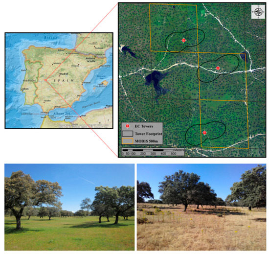
Figure 1.
Majadas experimental site (early spring in lower left panel and summer in lower right panel)) and location of the three EC towers (red points), with respective footprints delimited in black (60% iso-lines for the period of March 2014 until January 2017 and estimated according to Kljun et al. [46]). Selected MODIS 500m pixels for LAI estimations (Section 2.3.2) are highlighted in orange. The upper left panel reference map was created using ArcMap 10.3 online basemaps (ESRI. ´National Geographic’, http://www.arcgis.com/home/item.html?id=30e5fe3149c34df1ba922e6f5bbf808f, 13 December 2011).
2.2. TSEB Model Overview
The TSEB model was first proposed in Norman et al. [10], with important adjustments described in Kustas and Norman [14]. Its main inputs are LST, derived from thermal infrared (TIR) radiation, vegetation structural properties (e.g., LAI, canopy height), and meteorological forcing (irradiance, air temperature and wind speed). The principle source of uncertainty within TSEB lies in the estimation of the sensible heat flux (H), which is calculated through the heat transport equation (Equation (1)).
where H is sensible heat flux (W m−2); is the volumetric heat capacity of air (J m−3 K−1); is the aerodynamic temperature of the surface (K); is the air temperature at a reference/measurement height (K); and is the aerodynamic resistance to heat transport (s m−1). The heat transport equation is satisfied when using aerodynamic surface temperature (i.e., surface temperature at the canopy source-sink height), however, LST obtained from TIR remote sensing (i.e., skin radiometric surface temperature) can differ up to several degrees compared to the aerodynamic surface temperature [10], and their relationship is not well established (i.e., [47]). TSEB thus tackles this issue by assuming that the total blackbody thermal radiance that is emitted by the bulk surface is weighted by the fraction of vegetation observed by the sensor and the emission of both soil and vegetation surfaces, as expressed in Equation (2) taken from Norman et al. [10]:
where is the fraction of vegetation observed by the TIR sensor at zenith angle θ and is mainly a function of LAI; is the vegetation canopy temperature (K); and is the soil surface temperature (K). Using this two-layer approach, the energy balance is formulated in TSEB for each of the layers separately as follows:
where is the net radiation (W m−2); LE is latent heat flux (W m−2); G is the soil heat flux (W m−2); and subscripts s and c refer to soil and vegetation canopy sources, respectively. Note that horizontal heat advection, canopy heat storage as well as the energy used for CO2 fixation, are neglected in Equation (3). Radiative transfer and absorption through the canopy ( and ) are simulated through a radiative transfer model considering spectral differences in the visible, near-infrared and longwave radiation, multiple scattering between soil and canopy, and direct and diffuse irradiance, as described in chapter 15 of Campbell and Norman [48] and incorporated in TSEB by Kustas and Norman [14]. H is derived using an in ‘series’ resistance network [10] (Figure 2), and applying Equations (4)–(6), which allows for heat turbulent interchange between the canopy and soil layers:
where is the air temperature in the canopy space (K) and is equivalent to the aerodynamic temperature (); is the resistance to heat transfer in the boundary layer above soil layer (s m−1); is the bulk canopy resistance to heat transfer (s m−1); is the aerodynamic resistance to heat transfer based on the Monin-Obukhov similarity theory. Refer to Appendix A of Norman et al. [10] for details on the series resistance scheme.
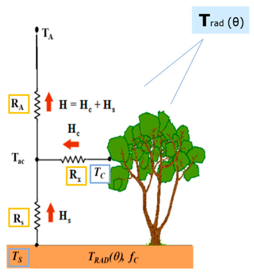
Figure 2.
TSEB Sensible Heat model scheme (adapted from Kustas and Anderson [9]).
Since Equation (2) has two unknowns ( and ), the canopy layer is assumed, as a first estimate, to be initially transpiring at a potential rate () using the Priestley–Taylor formulation:
where is the initial canopy transpiration estimate (W m−2); is the Priestley-Taylor coefficient (default is 1.26) (-), defined in this case only for the canopy component [9]; is the fraction of vegetation that is green and hence actively transpiring (-); ∆ is the slope of the saturation vapor pressure curve at air temperature Ta (kPa K−1); and γ is the psychrometric constant (kPa K−1). This initial assumption, where the canopy is transpiring without water stress (i.e., , is used to initialize the model, which allows to solve all the systems of equations presented above (Equations (2) to (7)). However, if the vegetation is stressed, the Priestley–Taylor formulation will overestimate the transpiration of the canopy and hence underestimate canopy temperature, which, in order to conserve the total surface temperature in Equation (2), will result in an overestimation of both soil temperature and soil sensible heat flux (i.e., Equation (4)). At this point, in order to preserve the energy balance in the soil (Equation (3)), would likely yield negative values, meaning soil condensation, which is unrealistic under daytime conditions. As it is assumed that condensation does not occur during daytime convective conditions, an iteration procedure is applied that reduces in small steps until realistic soil fluxes area achieved (i.e., ≥ 0). A more complete discussion on conditions that reduces is given in Anderson et al. [49] and Li et al. [39]. For more implementation details, the reader is referred to the source code (https://github.com/hectornieto/pyTSEB) and Norman et al. [10].
2.2.1. Radiation Transmission in Sparse Vegetation
The structure and distribution of foliage in the vegetative layer has an important impact on the dynamics of radiation interception and transmission through the canopy [14,49,50]. This in turn has a very important implication for radiometric temperature partitioning between the soil and vegetation components and their resulting contribution to heat fluxes [49]. The original TSEB radiative transfer equations assume a randomly distributed homogenous (i.e., non-clumped) canopy [10]. However, sparse vegetation is generally clumped and tends to intercept less radiation for the same foliage density compared to vegetation randomly dispersed over the surface [14,48]. As such, the clumping index (Ω) quantifies the spatial distribution of foliage to account for non-randomness in vegetated structures. LAI is multiplied by the clumping factor to obtain effective LAI (ΩLAI). As incorporated in Kustas and Norman [14]. TSEB estimates Ω as a function of the difference between the canopy gap fraction compared to a homogenous case using Equation (8) (Section 2 in Kustas and Norman [14]) and estimating the beam extinction coefficient assuming an ellipsoidal leaf angle distribution (LAD) with Equation (9) (Section 15.2 in Campbell and Norman [48]).
where Ω(0) is the clumping index when the vegetation canopy is viewed at nadir (-); is the beam extinction coefficient (-) based on a ellipsoidal LAD function (Campbell and Norman [48]); is the vegetation fractional cover (-); F is the local LAI (F = LAI/); and is the leaf inclination distribution function chi parameter (-) [48]. Ω is also dependent on the solar zenith angle () and is estimated using Equation (10), as described in Section 15.13 of Campbell and Norman [48].
where p = 3.8–0.46 (1/wc); and wc is the vegetation´s width to height ratio (-).
2.2.2. Resistances within and below Canopy
The semi-empirical derivations of and , as introduced in Norman et al. [10] and Kustas and Norman [14], are dependent on wind speeds below and within the vegetative canopy, respectively (Equations (11)–(12)).
where is the wind speed just above the surface where the impact of soil roughness is minimal (i.e., (ms−1); is the wind speed within the canopy-air interspace at the height of momentum source/sink (ms−1); is the effective leaf width size (m); and c (m s−1 K−1/3)), b (-) and C’ (s1/2 m−1) are coefficients taken from Kustas and Norman [14] and Norman et al. [10] based on the works of Sauer and Norman [51], Kondo and Ishida [52], and McNaughton and Van Den Hurk [53] (default values are 0.0025 m s−1 K−1/3, 0.012 and 90 s1/2 m−1 respectively). and in Equations (11) and (12) are both derived from an observed wind speed above the canopy that is extrapolated through and below the canopy based on the exponential wind attenuation law [54]. The two key roughness parameters, the zero-plane displacement height (d0) and the aerodynamic roughness length for momentum transfer (z0m) are estimated from the vegetation structure. When considering the grass canopy layer, the traditional fixed ratio to canopy height method is used to estimate d0 and z0m [48]. In the case of the tree canopy layer, a different approach is used (see Appendix B), which additionally considers the canopy shape and density´s effect on the roughness parameters. This study follows the procedure described in Schaudt and Dickinson [55], which stems from the work of Raupach [56] and Lindroth [57], and is generally viewed as more suitable for tall wooded vegetation. These methods do not apply corrections associated to the roughness sub-layer (e.g., Weligepolage et al. [58]). However, Alfieri et al. [37] found that the TSEB modelled fluxes were largely insensitive to differences in estimated d0 and z0m obtained from various methods in a vineyard. This is due to the fact that rougher surfaces, such as tall canopies, are better coupled to the atmosphere and, hence, the transport of heat and water vapour is more dominated by the canopy´s physiological mechanisms rather than aerodynamic roughness [59].
2.3. Data
2.3.1. Eddy Covariance and Bio-Meteorological Measurements
The three EC towers (CT-FLUXNET identifier ES-LMa, NT–FLUXNET ID ES-LM1, and NPT–FLUXNET ID ES-LM2), simultaneously operating within the Majadas study site, provided all necessary inputs to run TSEB (Table 1), except for continuous vegetation LAI estimates (Section 2.3.2). H and LE estimations from the EC system served to benchmark model performance. Details on the data processing are found in El-Madany et al. [43]. Data were obtained between the period of 2015-01-01 and 2017-12-31. Data which did not satisfy the assumptions of the EC methods [60] or with low turbulent conditions [61] were filtered from the dataset. Since TSEB forces the closure of energy balance (via Equation (3)), energy balance closure of the EC flux measurements was ensured by allocating the residuals to the observed LE, assuming that errors in LE are larger than H due to issues related to the instrumentation (i.e., Foken et al. [62]), as in previous studies (e.g., Guzinski et al. [63]; Kustas et al. [64]; Twine et al. [65]; Niaghi et al. [66]). Measurements from 2015 of the CT tower were selected as the ‘main’ simulation site/period and used to perform the SA (Section 2.4.2) and the main model runs (Section 2.4). Other towers (NT and NPT) and years (2016 and 2017) provided independent evaluations of model performance (Section 2.4.5).

Table 1.
Data used to parameterize and evaluate the TSEB model.
While TSEB has used different methods to estimate ground heat flux (G) (e.g., [10,67]), this study directly forced in situ G measurements as a model input to limit uncertainty and noise in turbulent flux estimations associated with errors in G. However, for the validation model runs, G was modeled with the time difference approach of Santanello and Friedl (Section 2.4.5). At each tower, the weighted average of eight soil heat flux plates, all buried at 5cm depth, represented G at the ecosystem level. Four of these were located in open grass and the other four plates were placed below the tree canopy. The weighted contributions of the plates below the tree and in open grass were estimated based on the solar zenith angle (SZA) throughout the day. At solar noon (i.e., SZA is 0 degrees), it is estimated that the tree canopy cover is 20% and that the plates in the shade below the trees contribute this same percentage (and the open grass plates contribute 80%). At sunset/sunrise (i.e., SZA > 85 degrees), the open grass area (i.e., non-shaded area) does not contribute to the ecosystem G. As such, the SZA is normalized between these two limits and used to scale the relative contribution between the soil heat flux plates buried below the tree canopy and those in the open grass. Note that corrections related to heat storage above the soil heat flux plates were not applied and, as such, G is likely slightly underestimated. The radiometric LST was estimated using proximal sensing from the CNR4 (Kipp & Zonen, Delft, Netherlands) longwave radiometers installed in the EC system (Equation (13)). These radiometers cover a footprint representing roughly 19-25% of tree cover for the three towers (i.e., CT, NT and NPT) used. These are very similar to the average tree contribution to the EC footprint reported in El-Madany et al. [43].
where and are upwelling and downwelling longwave radiance; is the Stephan-Boltzman constant; is the surface emissivity where leaf and bare soil broadband emissivity were taken as 0.99 and 0.94, respectively [68,69]. These broadband emissivity values were supported by computing broadband emissivity from typical soils and vegetation from the ECOSTRESS spectral library (https://speclib.jpl.nasa.gov/).
2.3.2. Vegetation Biophysical Measurements
In situ grass LAI measurements were acquired in the context of the FLUXPEC project (http://www.lineas.cchs.csic.es/fluxpec/) at eleven plots (25 m × 25 m) randomly placed around the CT in nineteen field campaigns between 2013-10-31 and 2016-11-16 [71]. Destructive samples were collected in two 25 cm × 25 cm quadrants within each plot and LAI was derived using gravitational methods, where green and non-green elements were separated to compute both total and green LAI. Time series of reflectance factors from the MODIS/Terra and Aqua Nadir BRDF-adjusted Reflectance Daily L3 500m v006 (MCD43A4) product were acquired for pixels centered in each of the three towers (Figure 1) [72]. The 500m by 500m pixel size was considered adequate to characterize the tower footprint. The normalized difference vegetation index (NDVI) was derived using band 1 (red: 620 nm–670 nm) and band 2 (NIR: 841 nm–876 nm) as follows:
An empirical relationship between NDVI and in-situ destructive grass LAI measurements was developed specifically for the Majadas experimental site (Appendix A, Figure A1). In order to obtain the ecosystem LAI adjusted for the tree canopy effect within the tower footprint (Figure 3), in-situ tree LAI measurements were incorporated to achieve a weighted average between tree (20%) and grass (80%) (Figure A2). The average tree LAI acquired using the LAI-2200 plant canopy analyzer (LAI-2200) (LICOR Bioscience USA, 2011) during five field campaigns at different seasonal periods between 2017-2018 was used as a reference. Local tree LAI ranges between 1.39 and 1.75 m2 m−2 (about 0.3 m2 m−2 effective/landscape LAI) and has low inter-annual variability [28]. Linear interpolation between sampling dates was performed to obtain a continuous daily time series (Figure A2).
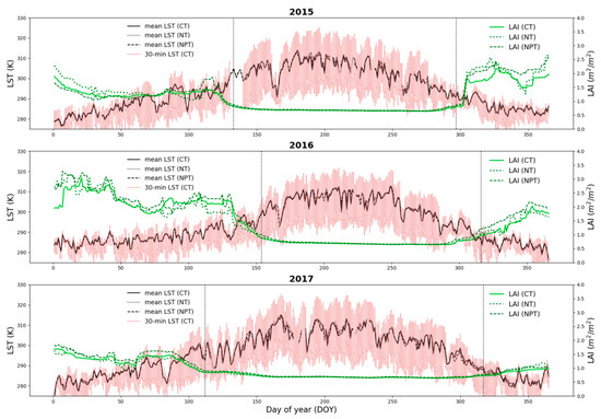
Figure 3.
Annual time series of half-hourly LST at CT (red), daily mean LST (black) and ecosystem LAI (green) for CT (solid), NT (dotted) and NPT (dashed) for 2015, 2016 and 2017. Vertical dotted lines indicate transition dates used for TSEB-2S (Section 2.4.4).
2.4. Model Simulations and Evaluation
Global and local SAs were performed on the main parameters and inputs, respectively using the default TSEB model (Section 2.4.1 and Section 2.4.2). In addition, two end member simulations, where either a pure grassland or broadleaf forest was assumed for the entire year, were performed to better understand the effect of the vegetation canopy on simulated fluxes for extreme cases (Section 2.4.3). The model was then adapted considering two distinct seasonal periods, each having a dominating vegetation layer (Section 2.4.4). All simulations were evaluated for daytime fluxes (i.e., when Sdn > 50 W m−2) since TSEB is designed to model fluxes for daytime conditions with remote sensing data (Section 2.4.5).
2.4.1. Default TSEB Model Configuration
In this default configuration (hereafter as TSEB-DF), the vegetated layer was parameterized attempting to depict the mix between tree and grass observed over tower footprint, where the vegetation cover was dominated by grass, but the turbulent resistances were assumed to be largely affected by the sparse tree layer [43]. As such, ecosystem LAI (weighted average of grass and tree LAI, Figure 3 and Figure A2) was used as input and vegetation resistances and roughness were derived using the weighted average of grass and tree canopy height ( = 0.8 × 0.5m + 0.2 × 8m = 2m). The roughness parameters were estimated following the procedure as described in Schaudt and Dickinson [55]. Table 2 summarizes the parameter values used for this default model configuration. The green fraction () was set to 0.7 being roughly the average value observed from grass field measurements. The model simulations were performed at the sub-hourly (30-min) time step for 2015 over the CT EC footprint and benchmarked against EC derived LE and H.
Table 2.
Parameter values of the TSEB-DF model configuration.
2.4.2. Sensitivity Analysis
Sobol´ Global Parameter Sensitivity Analysis
Variance-based SA methods decompose the total variance between simulated and observed data into various parts, determining the contribution of the different parameters and their combined interactions on total output variance. In this work, the Sobol’ SA method was used as it is able to compute the 1st, 2nd and total order sensitivity indices. To apply this methodology, a selection of model parameters and their respective bounds were configured (Table 3). Based on this, parameters sets for n simulations were generated using the Sobol´ sequence [40,41], a quasi-random method with quasi-Monte-Carlo integration.
where y is an indicator of the model performance and {} is the model parameter set which controls the model behavior and, thus, its performance, y. The Sobol’ approach decomposes the variance observed in y through the variance in all θ factors (Equation (15)) by separating parameters into terms of increasing dimensionality, with each successive dimension representing greater interaction of parameters, represented as:
where is the total output variance; is the portion of variance contributed by parameter (also known as the first order variance or main effect); and is the portion of variance attributed through the interaction between and and so on. The Equation (16) holds if all the parameter factors are independent [40], which is the case for this study. Parameter values do not correlate and are independently assigned over a uniform distribution between the specified bounds (Table 3).
Table 3.
Parameters bounds for the Sobol’ global SA.
The first-order sensitivity (), second-order sensitivity () and total order sensitivity () indices are calculated using Equations (17) to (19) as:
where is the average variance depicted when all parameters except for vary (i.e., is kept fixed); represents the contribution of both the direct (1st order) and indirect (sum of 2nd order) effects of on the total variance, .
Model variance was calculated based on H since LE is computed through the residual of the energy balance in TSEB, where errors in H are transposed into LE. Root-Mean-Square Deviation (RMSD) was used as the objective function to quantify model output variance for the entire simulation year, where tower-based EC H provided the observed time series.
where is modeled H at a 30 minutes time step; is the observed EC H; and N is the total number of observations used. The SA was undertaken with TSEB-DF, considering the 11 parameters within TSEB (i.e., second group of variables in Table 1), which are used in the sub-modules of radiation transfer between vegetation and soil (, and ) roughness and resistance scheme (), and the initial canopy transpiration estimate from the Priestley-Taylor formulation ( and ). Their respective bounds were based on literature or the physical limits of the parameter in question (Table 3). We note that the lower bound for = 1.26 is merely used as a first estimate for the model initialization. TSEB has an internal procedure to reduce due to conditions of stress, and, since no a priori information on stress is known, it is not recommended to use a value lower than 1.26 for model initialization [20]. A total of 45,500 simulations were used for this SA. The Python package SALib (Sensitivity Analysis Library in Python) [73] was integrated with the Python implementation of TSEB (pyTSEB, https://github.com/hectornieto/pyTSEB) to perform these analyses.
Input Local Sensitivity Analysis
Errors associated to the remote sensing derived input data (i.e., LST and LAI) are another important source to the total output uncertainty. Since input data are dynamic, a different method was needed compared to the static parameters described above for the global SA. Random white noise, mimicking potential errors of each input variable, over a uniform distribution of +-3K and +- 0.4 m2 m−2 were added to the ‘observed’ LST and LAI, respectively. The range of errors in LST was chosen to fit within the typical uncertainties associated with remote sensing based LST retrievals over vegetation (e.g., Sobrino et al. [74]). The range in LAI perturbation was based on the errors associated with the LAI empirical model used in this study (Appendix A, Figure A1). The sensitivity indices (SI) were then computed based on the partial derivative of the output result with respect to change in input caused by the implemented random noise, using Equation (21) adapted from van Griensven et al. [34].
where M is model output; refers to the different model inputs; refers to the pertubation of the input caused by artificial noise. The SI is based on the change observed for modeled H.
The input SA was implemented for 365 days (during 2015) with a 30-min time step. Since TSEB incorporates LAI at the daily time scale, the SI is derived based on the daily aggregated absolute change in H in relation to the absolute change in LAI for that day. For the LST analysis, the effect of a deviation in LST on the resulting H will likely be impacted by the time in which the deviation occurs (i.e., a perturbation in LST during morning time will likely impact H differently compared to a midday perturbation). To normalize the time of perturbation, for each simulation day, only the mean net perturbation of LST during midday (between 11:00 and 13:00 UTC) was used to analyze the net effect on H during that same time period. Hence, SIs for both LAI and LST were derived for each daily time step using the absolute change in inputs with the resulting absolute change in output (i.e., H).
2.4.3. End Member Simulations
In addition to the TSEB-DF simulations, two end member scenarios were conducted as limiting case studies. These type of end member configurations are typical for models applied to global remote sensing products, which often assign model parameter values (e.g., or which are typically more difficult to estimate directly) based on a specific or assumed land/vegetation type (e.g., [75]). However, errors in global land cover maps, which tend to be more common for TGEs (e.g., [24]), will cause for a less accurate parameterization and depiction of the surface conditions. For example, the Climate Change Initiative (CCI) land cover product [76] designates the Majadas study site as either ‘mosaic cropland’ or ‘mosaic herbaceous cover’. Therefore, these end member scenarios represent a similar or expected parameterization to the configurations applied for global scale energy flux products (e.g., [75,77]).
The first case assumes a pure grassland, ignoring the tree components, for the entire year (hereafter as TSEBgrass). The second case ignores the grass layer, simulating the vegetated component as a scattered evergreen broadleaf forest (hereafter as TSEBtree). The estimation of the roughness characteristics differed for each scenario as described in Section 2.2.2 (i.e., fixed ratio for grass layer and the method of Schaudt and Dickinson [55] when considering tree canopy) and the most influential parameters (as derived from the SA) were modified to characterize the assumed dominant vegetation with standard values (see Section 3.1.3). In addition, instead of ecosystem LAI, each end member scenario uses the LAI corresponding to the assumed vegetation layer (i.e., grass or tree LAI as shown in Figure A2). These end member scenarios were performed on the CT tower during 2015.
2.4.4. Two-Season Modeling Approach
We propose here an adaptation of the TSEB-DF by using a two-season modeling approach (hereafter as TSEB-2S) that divides the annual simulation into two main phenological periods: a grass dominated growing period (i.e., grass-soil system) and a tree dominated summer/dry period (i.e., tree-soil system). This modeling scheme attempts to depict the vast changes observed in TGE surface condition due to phenology. Phenological processes are important in this ecosystem [28] and these changes in vegetation cover alter the turbulent conditions (i.e., roughness), radiation transmission and, hence, the surface energy balance [29]. In semi-arid TGEs, during the summer period, the grass understory rapidly transforms into a dry and rough layer with minimal transpiration from vegetation. Therefore, the TSEB-2S separates the simulation period for these two major conditions observed: 1) the grass is active and transpiring (growing season) and 2) the grass species are senesced and not transpiring (summer), neglecting any transition period between seasons due to the rapid grass senescence period that characterize semi-arid TGEs [28]. The transition dates were estimated using an asymmetric gaussian filter over the MODIS (MCD43A4 product) derived NDVI time series, where the dry period was assumed to begin when vegetation (i.e., NDVI) begins to decay (downward inflection point) and the dry period ends when vegetation (i.e., NDVI) begins to re-green (upward inflection point). For instance, for the simulation year of 2015, the dry period begins on May 13th and ends on October 24th (refer to Figure 3 for all transitions dates used). As such, this method can be a general and automatic approach to derive the seasonal transition dates at the global scale, which may be applied to other TGE or semi-arid sites with marked seasonality.
2.4.5. Model Evaluation
TSEB-2S was evaluated using independent model simulations for different spatial (three tower sites) and temporal (three different years) characteristics. The benchmark simulation run (i.e., TSEB-DF) and the SA were forced with observed G to limit the noise and uncertainties related to the errors in estimated G. This way we can more accurately pinpoint the uncertainties related to the H (and, by consequence, LE) retrievals. However, the model validation runs were performed by modeling G using the approach of Santanello and Friedl instead of using observed G. This was implemented to better evaluate the model in a more operational setting, where remote sensing-based retrievals may not have in-situ G measurements available. Model performance was evaluated against the observed EC tower measurements in question and quantified with RMSD (Equation (20)), mean bias (Equation (22)) and the Pearson´s correlation coefficient (r).
Additionally, an evaluation of the modeled LE partitioning, between LEc and LEs, was performed. Since TSEB-2S assumes a different and unique vegetation structure and cover for different seasonal periods, it was interesting to evaluate if the model can also obtain reliable estimates of the LE partitioning along with the bulk fluxes. Modeled LEs was evaluated against independent lysimeter LE measurements (LElys) of the understory during the dry summer periods at CT, when the grass is senesced and, thus, LElys is assumed to be equivalent to soil evaporation (i.e., LEs). For a detailed description of the lysimeter set-up in the Majadas experimental site, refer to Perez-Priego et al. [42].
3. Results
3.1. Sensitivity Analysis
3.1.1. Global Sobol´ Parameter SA
The parameter global SA showed that had the largest impact on model results, both as the main effect (Si) and through its interactions with other parameters (ST) (Figure 4). In general, parameters related to vegetated structure () and cover ( and ) demonstrated the largest sensitivity. Notably, many parameters had low first order sensitivities (close to 0) but relatively important total order sensitivities, indicative of large interactions between parameters. The b parameter, used in the computation of , was the only more empirically derived parameter that demonstrated a relatively high influence on modelled output.
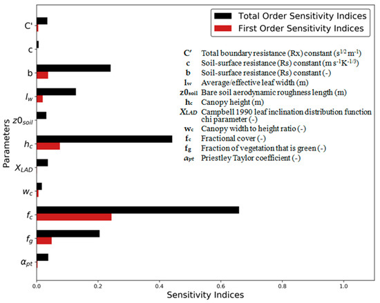
Figure 4.
First (Si) and total (ST) order SI for the main parameters in TSEB-DF.
3.1.2. Local Input SA
Uncertainties related to LST and LAI showed important impacts on model results (Figure 5). Simulated H is particularly sensitive to deviations in LST, where differences of a unit change of LST (∆ 1K) is associated to a median 17.3% change in modelled H. The uncertainty in LAI demonstrated, compared to LST, relatively less influence on H. A 0.1 m2/m2 change in LAI is associated with a 2.9% change in simulated H with TSEB-DF.
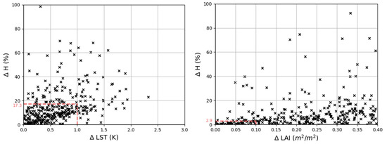
Figure 5.
Scatter plots of the absolute percent change in daily aggregated H (y-axis) with the associated absolute perturbation of the daily aggregated input (x-axis): LST (left) and LAI (right) using TSEB-DF. The median percent change in modelled H for a 1K change in LST (left) and a 0.1 m2/m2 change in LAI (right) are shown as dashed red lines.
3.1.3. TSEBgrass, TSEBtree and TSEB-2S Model Configuration
The global SA results illustrated in Figure 4 showed that parameters related to the vegetation cover (i.e., and ) and structure (i.e., ) had the most influence on model performance. Since these are physical and measureable parameters, these were set for each end-member scenario (Section 2.4.3) according to the assumed dominant vegetation as described in Table 4. The was set to 0.7 for the grass configuration according average field observations, while it was set to 0.9 for the evergreen tree cover to account for the presence of non-photosynthetic material such as branches. The for the tree layer was set to 8 m according to the mean height of trees within the study site [43] and its was set 0.2, this being about the average tree canopy fraction observed for the tower footprints [43]. Additionally, the was increased to 0.05 m for the tree cover to better represent the larger leaves of the oak species (compared to the grass species) within the study site. The resistance b coefficient, used in the formulation of , was increased for the scattered tree cover, as was successfully tested and implemented in Kustas et al. [21] to better simulate rough surfaces and partially vegetated surfaces. The b parameter was given a value of 0.034 for the tree-soil summer period, based on the range reported in Sauer et al. [70] for partial vegetation conditions [21,70]. Other parameters, such as , which is presumably different between grasses and trees, were not modified since they showed little sensitivity (Figure 4).
Table 4.
TSEBgrass and TSEBtree model configurations based on global SA.
To improve the seasonal depiction and related changes to the ecosystem, the TSEB model was adapted using a two-season modelling approach (TSEB-2S) as described in Section 2.4.4. The simulation was divided into two main phenological periods where a dominant vegetation is assumed in each case and TSEB is parameterized according to the respective end-member parameter values shown in Table 4 (i.e., TSEBgrass during the growing season and TSEBtree during the dry summer).
3.2. Model Evaluations for Main Simulation Period (2015 CT)
TSEB-DF, the end-member configurations (TSEBgrass, TSEBtree), and TSEB-2S were all first evaluated against EC measurements from CT for the entire year of 2015. Figure 6 shows the TSEB-DF modelled vs. observed half hourly turbulent fluxes as well as the annual trend of daytime average sensible heat flux, both modeled and observed. Model results of TSEB-DF vastly underestimate H (bias: -45 W m−2) and, consequently, overestimate LE (bias: 40 W m−2) as compared with observed EC data. As shown in Figure 6 (left panel), high errors are observed throughout (RMSD of H: 82 W m−2) but errors stem particularly from the very large underestimations of H during the hot and dry summer period (Figure 6, right panel). TSEB-DF was attempted to be parameterized as a mixed layer between tree and grass vegetation. However, it was not able to accurately reproduce LE (and H) largely because its parameterization was not able to consider the drastic change occurring during the summer, where roughly 80% of surface cover (i.e., grass understory) becomes non-physiologically active and, thus, non-transpiring.
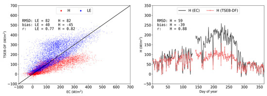
Figure 6.
Observed vs modeled daytime half-hourly H (red) and LE (blue) density scatterplot (left) and time series of simulated (red) and observed (black) daytime daily mean H (right) for TSEB-DF in 2015 at CT.
The end member simulations demonstrate the ‘boundary conditions’ when the simulations completely ignored one of the vegetation layers throughout the year (Figure 7). Predictably, TSEBgrass, underestimates H even more than TSEB-DF (bias: −54 W m−2), while, by contrast, LE is largely underestimated in TSEBtree (bias: −23 W m−2), with large errors (RMSD: 82 W m−2). Both TSEBgrass and TSEBtree performed poorly because they do not adequately depict the surface conditions for the different phenological periods with one of the two major vegetation covers being ignored throughout the year. TSEBtree performed slightly better compared to TSEBgrass because it better captured the conditions and fluxes for the summer drought season, which was the period with the largest biases and uncertainties.
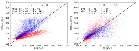
Figure 7.
Observed vs modeled half-hourly daytime H (red) and LE (blue) density scatterplot for TSEBgrass (left) and TSEBtree (right) for 2015 at CT.
The performance of the proposed TSEB-2S parameterization is shown in Figure 8. The simulation of LE and H for 2015 improved considerably when using TSEB-2S compared to TSEB-DF (and end-members). Errors with TSEB-2S decreased substantially (decrease in RMSD from 82 W m−2 to 59 W m−2 and 55 W m−2 for LE and H, respectively) and the seasonal average daily H was much improved, particularly during the summer/dry period (RMSD of daily mean H decreased from 59 W m−2 to 26 W m−2). TSEB-2S allowed different parameterizations to be applied according to the assumed ‘dominant’ vegetation structure and cover in contrasting phenological periods observed in TGEs. All metrics for model performance improved with the use of TSEB-2S. RMSD and bias decreased substantially compared to TSEB-DF and the correlation (i.e., r) between modeled and observed data increased. However, the winter-autumn period (roughly between DOY 25 and 125) still showed a slight systematic H underestimation with TSEB-2S similar to TSEB-DF.
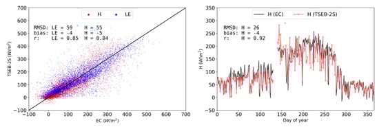
Figure 8.
Observed vs modeled daytime half-hourly H (red) and LE (blue) density scatterplot (left) and time series of simulated (red) and observed (black) daytime daily mean H (right) for TSEB-2S simulations of 2015 at CT.
3.3. TSEB-2S Validation
TSEB-2S substantially improved estimated fluxes compared to the default implementation of TSEB (TSEB-DF). To further validate this modeling strategy, TSEB-2S was tested independently for different years (2016 and 2017) with very different intra-annual dynamics, and against two other EC towers (NT and NPT) within the experimental site (using the same meteorological forcing). In addition to evaluating the bulk fluxes, the LE partitioning between soil evaporation and transpiration was evaluated using lysimeter measurements at the CT.
3.3.1. Independent Evaluations for 2016 and 2017 over CT, NT and NPT Towers
TSEB-2S was tested for all EC towers (CT, NT and NPT) in 2016 and 2017. The results from these other towers and years (Figure 9) were within similar error ranges to the benchmark TSEB-2S 2015 simulation at the CT. RMSD and bias for LE, in all validating simulations, range between 57 and 63 W m−2 and −2 and −12 W m−2, respectively. This range in error is very much in line to the benchmark simulation period even though modeled, rather than observed, G was implemented. The available energy (AE), Rn – G, was also generally well modeled for all model runs (Figure A3).
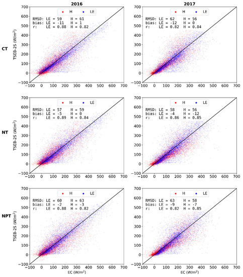
Figure 9.
Observed vs modeled daytime half-hourly H (red) and LE (blue) density scatterplot for TSEB-2S for CT, NT and NPT; and years 2016 (left column) and 2017 (right column).
3.3.2. LE Partitioning
The LE partitioning in TSEB-2S was evaluated against independent estimates from the lysimeter at the CT footprint during the summer drought, when there is no grass transpiration and, thus, LE measured by the lysimeter (LElys) corresponds to soil evaporation [30,42]. Results indicate a general, slight LEs underestimation during the dry period for the three years analyzed (Figure 10). Additionally, important errors stem from the greater short-term variability of the modeled fluxes compared to the relatively stable lysimeter measurements. The LEs underestimation (bias: −18 W m2) and errors (RMSD: 41 W m2) were largest for 2016. The larger errors during this year were partly explained by the greater underestimation from the dry-down period (roughly DOY170-185), which is also apparent, while less substantial, for 2015. As shown in Figure 10, modeled LEs had a much more rapid decrease in magnitude compared to the gradual decrease observed from the lysimeter during this dry-down period. TSEB-2S was able to capture the temporal dynamics and evaporation peaks relatively well but the dry-down after the rare rainfall events was also more gradual in the observed lysimeter compared to the modeled fluxes. This may be explained by the evaporation being sustained from the deeper soil, which is more difficult to capture from the model since it is forced with the ‘skin’ radiometric surface temperature (i.e., LST).
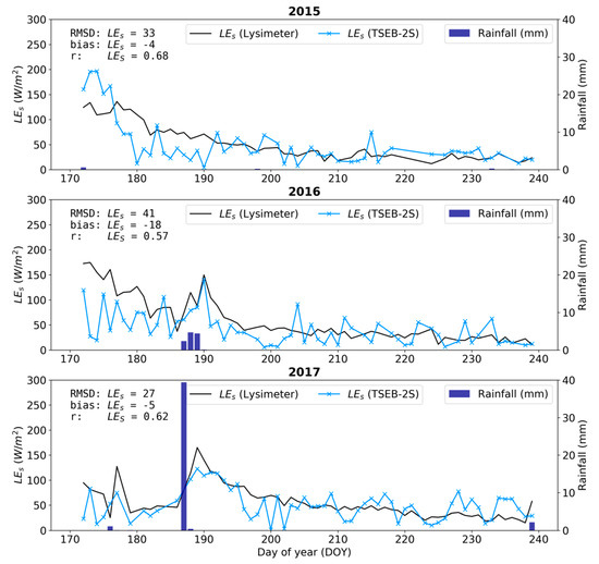
Figure 10.
Time series of simulated (blue) and observed (black) daytime daily mean LEs at CT during the peak summer in 2015, 2016 and 2017 using TSEB-2S. LE measured by the lysimeter is assumed to be equivalent to LEs during the summer period due to grass senescence.
4. Discussion
The proposed TSEB-2S vastly improved model performance in simulating LE and H compared to the default TSEB configuration (RMSD and bias of modelled H decreases from 82 and −45 W m−2 to 55 and −5 W m−2, respectively). The simple assumption of two separate phenological and modelling periods, one dominated by a grass-soil system and the other dominated by a tree-soil system, allowed for a two-layer model to accurately simulate turbulent energy fluxes in an essentially three (tree-grass-soil) layer ecosystem. TSEB assumes only one vegetated layer, being more or less photosynthetically active, over a non-photosynthetically active layer (i.e., bare soil or similar). Therefore, it becomes difficult to properly parameterize the model when numerous vegetation covers are simultaneously present. Additionally, as in the case of many TGEs, the influence of the grass understory changes throughout the year, where it becomes largely non-photosynthetically active (i.e., not transpiring) during the summer. Therefore, these vastly different seasonal conditions and characteristics were better captured using TSEB-2S, by assuming a ‘dominant’ vegetation cover for different phenological periods, compared to the default, single mixed vegetation, configuration of TSEB (TSEB-DF). The relatively simple and automatic separation of seasons from a MODIS-NDVI time series can easily be extrapolated to other TGEs or similar temporally dynamic sites, as these data are globally available. The results also demonstrate that large changes to the vegetated surface have a considerable influence on the surface energy balance. This confirms the importance of vegetation characteristics in controlling and mediating ecosystem level energy fluxes, where seasonal dynamics and phenology of vegetation are key considerations for land-atmospheric modelling. The findings presented here describe a relatively simple and general approach to account for changes in land-atmospheric exchanges due to phenology such as those occurring in semi-arid TGEs. In this regard, a similar strategy can be implemented in other global soil-vegetation-atmosphere-transfer (SVAT) or prognostic models to better accommodate seasonality for ecosystems with comparable characteristics.
The TSEB-2S model demonstrated robustness, being able to accurately simulate different intra-annual dynamics for various years (i.e., different phenological timings) and sites with differing surface conditions, in this case, derived from a nutrient fertilization experiment (Figure 9). Results and the associated magnitudes of errors for all TSEB-2S model runs are similar to the error bounds found in other energy balance model studies (e.g., [14,15,21,22,38,63,78]) and close to the typical uncertainty of surface turbulent flux measurement systems (i.e., ~50 W m−2; [79]). For instance, RMSD of LE between 62 and 70 W m−2 were achieved by Timmermans et al. [23], who compared the use of TSEB against a one-source energy balance model for a sparsely vegetated grassland and rangeland. In the work of Boulet et al. [78], different dual-source model schemes were tested and obtained an RMSD between 53 and 73 W m−2 for midday instantaneous LE for both irrigated and rainfed wheat fields. Therefore, the results presented here, are in line with past studies related to LE retrievals, with these considering much more homogeneous land cover types, which better fit the assumptions inherent in SEB models compared to the multiple and more structurally complex vegetation cover in TGEs. Andreu et al. [31] applied various modified versions of TSEB, notably with different wind profiles and roughness schemes, in similarly complex TGEs and reported errors between 44 and 60 W m−2 for simulated LE. These are comparable to the error bounds presented here even though quite different approaches were used. In our study, the basic TSEB model structure was not modified, instead opting to alter the model parameterization depending on the phenological period using typical land cover characteristics (i.e., grasslands and evergreen broadleaved trees). As such, the findings here may complement the methods used by Andreu et al. [31], who also reported the largest errors during the dry, summer period.
The global SA demonstrated that TSEB was most sensitive to . This is largely due to being a key input to estimate the Ω (Kustas and Norman [14]), which in turn affects the radiation interception and partitioning between the mixed vegetated and soil surfaces. The estimation of Ω is mostly based on the transmission through the vegetated layer where is used to obtain a local LAI (LAI/) and as an important weighting factor for the gap fraction estimation (Section 2.2.1). These results are largely in line with results from Li et al. [39], who found that the Ω uncertainties had a large impact on flux outputs from TSEB. They tested incremental values, between 0.1 and 1, that resulted in sharp H changes, particularly between higher values, an indication of a high sensitivity for this parameter. The was found to be more sensitive compared to even though both parameters are part of the initial canopy transpiration estimate from the Priestly-Taylor formulation (Equation (7)). This is the case since is merely used as a priori estimate for initializing the model and is gradually decreased when there are conditions of water stress, until the energy balance is achieved with realistic daytime fluxes using LST as a boundary condition (as previously discussed in [10,78]). Figure A4 shows the daily average trend for the retrieved effective with TSEB-2S at CT in 2015. Note in Figure A4 that (defined for only the canopy source i.e., Kustas and Anderson [9]) maintains closer to the initial value of 1.26 during the dry summer period since TSEB-2S is simulating the canopy transpiration as a scattered broadleaved evergreen tree cover, which has extensive root system able to withdraw water even under drought conditions. The b coefficient, used to estimate the soil resistance to heat transport (i.e.,), was the only more empirically derived parameter that demonstrated a relatively large influence on model results. However, no significant relationship (Figure A5A, r = 0.01) was obtained between and errors (i.e., residuals) in modelled H and a very small relationship between (canopy boundary resistance) and errors in H was found (Figure A5B, r = −0.19). The latter is likely caused by uncertainties in tree LAI, as is inversely proportional to LAI since the canopy is considered as a set of single-leaf resistors placed in parallel.
The input SA showed that uncertainties in LST and LAI both translate into uncertainties in modeled H. However, model results were found to be much more sensitive to LST compared to LAI. Gan and Gao [38] also found TSEB to be sensitive to biases in LST, where a 1K change is associated with median daily ~12–25 W m−2 bias. A local LAI SA in Li et al. [39] added +-20% deviation to LAI and investigated the associated relative H change in TSEB. Their associated ~3–8% bias in modeled H is similar to the results presented here, with a 20% change in LAI being associated with a median H bias of 6.1% with TSEB-DF. As such, the more comprehensive SA analysis presented here, considering parameter interaction in the global SA combined with a local input SA, were largely in line with results presented in different local and parameter specific SAs from the literature. These results will be useful for future studies, as we quantified the relative influence of the different modeling components in TSEB, which may be similar for other thermal-based energy balance models.
This work additionally investigated the partitioning of LE, which is a complex process to separate in ecosystems that have multiple vegetation layers. As shown, bulk (soil + vegetation) fluxes were well modeled in TSEB-2S for different years and towers. However, the partitioning of LE had greater uncertainty, with biases observed comparing modeled LEs to the lysimeter measurements (Figure 10). Since total LE was well modeled, this indicates errors associated with the partitioning itself. This may be due to TSEB interpreting moderately stressed vegetation with a moist soil as fully transpiring vegetation with a dry soil. However, the partition of LE is largely controlled through LAI within TSEB [17]. The poorer performance in the LE partitioning could be due to the assumed vegetation cover of the two different seasons not properly depicting the complex vegetation characteristics observed, affecting net radiation partitioning, notably during the growing season when the tree layer is neglected. TSEB’s relatively poor performance in partitioning LE was also observed over a vineyard in Kustas et al. [17]. As stated in Kustas et al. [17], more studies need to evaluate whether the poor partitioning is linked to uncertainties in input values (i.e., LAI) or biases caused by the modelling structure itself (i.e., initial potential canopy transpiration, radiation transfer).
As demonstrated, a simple adaptation to the modelling scheme in TSEB, depicting the phenological change in the vegetation source, were able to successfully simulate LE and H in a complex ecosystem. However, certain limitations are still present including the slight systematic underestimation of H during the grass growing season, particularly visible in the 2015 daily H time series (Figure 8). This is likely due to the modeling scheme in this period ignoring the effect of the tree canopy layer on the turbulent transport and hence on the calculation of the aerodynamic resistances. Compared to grasslands, tree canopies are more aerodynamically coupled to the atmosphere and hence their aerodynamic resistance is lower, resulting in that trees can dissipate heat more efficiently [43]. As discussed by El-Madany et al. [43], tree canopies in the Majadas experimental site were an additional H source, even though they tend to have a lower LST than the grass layer. As such, ignoring the tree canopy during the growing periods may not adequately represent the turbulent transport characteristics of the ecosystem, resulting in H underestimations, in some cases. On the other hand, neglecting the tree canopy during the growing season was supported by the evidence that the understory layer dominates LE in this site (as shown by Perez-Priego [42]). This may explain why TSEB-2S was largely capable to accurately model LE during this seasonal period for the different years assessed. Further adaptations to the TSEB model scheme may be needed for the more operational and larger scale use of this model, notably for similarly complex ecosystems such as TGEs. The differences between soil, grass, and tree layers should inherently be integrated within the modelling structure to robustly consider their different geometric, aerodynamic, and phenological properties and their resulting effect on energy fluxes.
5. Conclusions
When accounting for different phenological periods through an automatic vegetation seasonal change detection using a MODIS time series analysis, the TSEB model provided robust LE and H estimations for a three-layered heterogeneous and semi-arid TGE using a combination of satellite (LAI) and proximal (LST) sensors. This, in conjunction with the SA, confirms the important role that vegetation characteristics, notably its structure (i.e., ) and cover (i.e., and ), have on ecosystem level energy fluxes. The was the single most influential parameter on model performance, largely due to its role in characterizing vegetation clumping and how this, in turn, interacts significantly with other parameters. In addition, the uncertainties related to the traditionally remotely sensed derived inputs, notably LST, showed an important influence on output uncertainties.
The LE partitioning, between canopy and soil, showed a larger bias compared to the bulk fluxes. Based on this, further research should focus on the understanding of the radiation partitioning between the canopy and soil layers, and particularly, inherently accounting for the important differences between soil, grass, and tree layers of TGEs within the modeling structure. However, the relative simplicity of TSEB-2S has the potential to be applied with both satellite and/or airborne data over similarly complex landscapes in different regions. This may provide a simple solution to improve remote sensing-based flux products over semi-arid TGEs and other savanna-like ecosystems, which often assume a homogeneous vegetation layer.
Author Contributions
All authors contributed to discussing and improving the manuscript. M.P.M., H.N., D.R. and V.B.-L. designed and formulated the research. M.M. and A.C. designed the experimental infrastructure. V.B.L. analysed the data, created the figures and wrote the manuscript. A.C., M.M., T.S.E.-M. collected eddy covariance and biomet data. O.P.-P. collected, processed and provided lysimeter data. M.P.M. sampled and analyzed field LAI samples. All authors have read and agreed to the published version of the manuscript.
Funding
The research received funding from the European Union’s Horizon 2020 research and innovation programme under the Marie Sklodowska-Curie grant agreement No 721995. It was also funded by Ministerio de Economía y Competitividad through FLUXPEC CGL2012-34383 and SynerTGE CGL2015-G9095-R (MINECO/FEDER, UE) projects. The research infrastructure at the measurement site in Majadas de Tiétar was partly funded through the Alexander von Humboldt Foundation, ELEMENTAL (CGL 2017-83538-C3-3-R, MINECO-FEDER) and IMAGINA (PROMETEU 2019; Generalitat Valenciana).
Acknowledgments
We would to thank the all the anonymous reviewers for their comments and suggestions throughout the revision phase. The authors also acknowledge all colleagues and members of the FLUXPEC and SynerTGE projects for their help during the field campaigns and laboratory post-processing.
Conflicts of Interest
The authors declare that they have no conflict of interest.
Appendix A

Figure A1.
Empirical model between MODIS (MCD43A4) NDVI and in-situ destructive grass LAI measurements developed for Majadas experimental site.

Figure A2.
Grass, tree, and ecosystem LAI time series for the CT tower for 2015. Note that tree LAI shown here refers to the effective (landscape) LAI, meaning that the tree-based measurement was weighted by its fractional cover (i.e., 0.2).

Figure A3.
Observed vs modeled daytime half-hourly available energy (AE) [Rn – G] density scatterplot for TSEB-2S for CT, NT and NPT; and years 2016 (left column) and 2017 (right column).

Figure A4.
Time series of daily daytime average of retrieved effective with TSEB-2S for 2015 at the CT.

Figure A5.
Rs (A) and Rx (B) vs residual H error for TSEB-2S at the CT in 2015.
Appendix B
The roughness parameters (i.e., z0m and d0) for the tree canopy are estimated following the procedure described by Schaudt and Dickinson [55]. The reader is also referred to the source code of pyTSEB (https://github.com/hectornieto/pyTSEB/). The roughness parameters are estimated as follows:
where , is the vegetation fractional cover (-), is the canopy width to height ratio (-).
The Lindroth [57] correction factors, fz and fd for z0m and d0m respectively, are then implemented as:
where LAI is the leaf area index (-).
z0m and d0 are then calculated as:
where is the canopy height (m).
References
- Bonan, G.B.; Doney, S.C. Climate, ecosystems, and planetary futures: The challenge to predict life in Earth system models. Science 2018, 359, eaam8328. [Google Scholar] [CrossRef] [PubMed]
- Krinner, G.; Viovy, N.; de Noblet-Ducoudré, N.; Ogée, J.; Polcher, J.; Friedlingstein, P.; Ciais, P.; Sitch, S.; Prentice, I.C. A dynamic global vegetation model for studies of the coupled atmosphere-biosphere system. Glob. Biogeochem. Cycles 2005, 19. [Google Scholar] [CrossRef]
- Richardson, A.D.; Keenan, T.F.; Migliavacca, M.; Ryu, Y.; Sonnentag, O.; Toomey, M. Climate change, phenology, and phenological control of vegetation feedbacks to the climate system. Agric. For. Meteorol. 2013, 169, 156–173. [Google Scholar] [CrossRef]
- Stoy, P.C.; El-Madany, T.; Fisher, J.B.; Gentine, P.; Gerken, T.; Good, S.P.; Liu, S.; Miralles, D.G.; Perez-Priego, O.; Skaggs, T.H. Reviews and syntheses: Turning the challenges of partitioning ecosystem evaporation and transpiration into opportunities. Biogeosci. Discuss. 2019, 10, 3747–3775. [Google Scholar] [CrossRef]
- Jasechko, S.; Sharp, Z.D.; Gibson, J.J.; Birks, S.J.; Yi, Y.; Fawcett, P.J. Terrestrial water fluxes dominated by transpiration. Nature 2013, 496, 347. [Google Scholar] [CrossRef]
- Ershadi, A.; McCabe, M.F.; Evans, J.P.; Walker, J.P. Effects of spatial aggregation on the multi-scale estimation of evapotranspiration. Remote Sens. Environ. 2013, 131, 51–62. [Google Scholar] [CrossRef]
- Li, Y.; Huang, C.; Hou, J.; Gu, J.; Zhu, G.; Li, X. Mapping daily evapotranspiration based on spatiotemporal fusion of ASTER and MODIS images over irrigated agricultural areas in the Heihe River Basin, Northwest China. Agric. For. Meteorol. 2017, 244–245, 82–97. [Google Scholar] [CrossRef]
- Kalma, J.D.; McVicar, T.R.; McCabe, M.F. Estimating land surface evaporation: A review of methods using remotely sensed surface temperature data. Surv. Geophys. 2008, 29, 421–469. [Google Scholar] [CrossRef]
- Kustas, W.P.; Anderson, M.C. Advances in thermal infrared remote sensing for land surface modeling. Agric. For. Meteorol. 2009, 149, 2071–2081. [Google Scholar] [CrossRef]
- Norman, J.M.; Kustas, W.P.; Humes, K.S. Source approach for estimating soil and vegetation energy fluxes in observations of directional radiometric surface temperature. Agric. For. Meteorol. 1995, 77, 263–293. [Google Scholar] [CrossRef]
- Bastiaanssen, W.G.M.; Menenti, M.; Feddes, R.A.; Holtslag, A.A.M. A remote sensing surface energy balance algorithm for land (SEBAL). 1. formulation. J. Hydrol. 1998, 212, 198–212. [Google Scholar] [CrossRef]
- Su, Z. The surface energy balance system (SEBS) for estimation of turbulent heat fluxes. Hydrol. Earth Syst. Sci. Discuss. 2002, 6, 85–100. [Google Scholar] [CrossRef]
- Allen, R.; Tasumi, M.; Trezza, R. Satellite-Based energy balance for mapping evapotranspiration with internalized calibration (METRIC)\97Model. J. Irrig. Drain. Eng. 2007, 133, 380–394. [Google Scholar] [CrossRef]
- Kustas, W.P.; Norman, J.M. Evaluation of soil and vegetation heat flux predictions using a simple two-source model with radiometric temperatures for partial canopy cover. Agric. For. Meteorol. 1999, 94, 13–29. [Google Scholar] [CrossRef]
- Gonzalez-Dugo, M.P.; Neale, C.M.U.; Mateos, L.; Kustas, W.P.; Prueger, J.H.; Anderson, M.C.; Li, F. A comparison of operational remote sensing-based models for estimating crop evapotranspiration. Agric. For. Meteorol. 2009, 149, 1843–1853. [Google Scholar] [CrossRef]
- Guzinski, R.; Anderson, M.C.; Kustas, W.P.; Nieto, H.; Sandholt, I. Using a thermal-based two source energy balance model with time-differencing to estimate surface energy fluxes with day-night MODIS observations. Hydrol. Earth Syst. Sci. 2013, 17, 2809–2825. [Google Scholar] [CrossRef]
- Kustas, W.P.; Alfieri, J.G.; Nieto, H.; Wilson, T.G.; Gao, F.; Anderson, M.C. Utility of the two-source energy balance (TSEB) model in vine and interrow flux partitioning over the growing season. Irrig. Sci. 2019, 37, 375–388. [Google Scholar] [CrossRef]
- Nieto, H.; Kustas, W.P.; Torres-Rúa, A.; Alfieri, J.G.; Gao, F.; Anderson, M.C.; White, W.A.; Song, L.; Alsina, M.M.; Prueger, J.H.; et al. Evaluation of TSEB turbulent fluxes using different methods for the retrieval of soil and canopy component temperatures from UAV thermal and multispectral imagery. Irrig Sci. 2019, 37, 389–406. [Google Scholar] [CrossRef]
- Diarra, A.; Jarlan, L.; Er-Raki, S.; Le Page, M.; Aouade, G.; Tavernier, A.; Boulet, G.; Ezzahar, J.; Merlin, O.; Khabba, S. Performance of the two-source energy budget (TSEB) model for the monitoring of evapotranspiration over irrigated annual crops in North Africa. Agric. Water Manag. 2017, 193, 71–88. [Google Scholar] [CrossRef]
- Agam, N.; Kustas, W.P.; Anderson, M.C.; Norman, J.M.; Colaizzi, P.D.; Howell, T.A.; Prueger, J.H.; Meyers, T.P.; Wilson, T.B. Application of the Priestley-Taylor approach in a two-source surface energy balance model. J. Hydrometeor. 2010, 11, 185–198. [Google Scholar] [CrossRef]
- Kustas, W.P.; Nieto, H.; Morillas, L.; Anderson, M.C.; Alfieri, J.G.; Hipps, L.E.; Villagarcía, L.; Domingo, F.; García, M. Revisiting the paper “Using radiometric surface temperature for surface energy flux estimation in Mediterranean drylands from a two-source perspective”. Remote Sens. Environ. 2016, 184, 645–653. [Google Scholar] [CrossRef]
- Li, Y.; Kustas, W.P.; Huang, C.; Nieto, H.; Haghighi, E.; Anderson, M.C.; Domingo, F.; Garcia, M.; Scott, R.L. Evaluating soil resistance formulations in thermal-based two-source energy balance (TSEB) model: Implications for heterogeneous semiarid and arid regions. Water Resour. Res. 2019, 55, 1059–1078. [Google Scholar] [CrossRef]
- Timmermans, W.J.; Kustas, W.P.; Anderson, M.C.; French, A.N. An intercomparison of the surface energy balance algorithm for land (SEBAL) and the two-source energy balance (TSEB) modeling schemes. Remote Sens. Environ. 2007, 108, 369–384. [Google Scholar] [CrossRef]
- Jung, M.; Henkel, K.; Herold, M.; Churkina, G. Exploiting synergies of global land cover products for carbon cycle modeling. Remote Sens. Environ. 2006, 101, 534–553. [Google Scholar] [CrossRef]
- Cleugh, H.A.; Leuning, R.; Mu, Q.; Running, S.W. Regional evaporation estimates from flux tower and MODIS satellite data. Remote Sens. Environ. 2007, 106, 285–304. [Google Scholar] [CrossRef]
- Friedl, M.A.; Sulla-Menashe, D.; Tan, B.; Schneider, A.; Ramankutty, N.; Sibley, A.; Huang, X. MODIS Collection 5 global land cover: Algorithm refinements and characterization of new datasets. Remote Sens. Environ. 2010, 114, 168–182. [Google Scholar] [CrossRef]
- Schnabel, S.; Dahlgren, R.A.; Moreno-Marcos, G. Soil and water dynamics. In Mediterranean Oak Woodland Working Landscapes: Dehesas of Spain and Ranchlands of California; Campos, P., Huntsinger, L., Oviedo Pro, J.L., Starrs, P.F., Diaz, M., Standiford, R.B., Montero, G., Eds.; Landscape Series; Springer: Dordrecht, The Netherlands, 2013; pp. 91–121. ISBN 978-94-007-6707-2. [Google Scholar]
- Luo, Y.; El-Madany, T.; Filippa, G.; Ma, X.; Ahrens, B.; Carrara, A.; Gonzalez-Cascon, R.; Cremonese, E.; Galvagno, M.; Hammer, T. Using near-infrared-enabled digital repeat photography to track structural and physiological phenology in Mediterranean tree-grass ecosystems. Remote Sens. 2018, 10, 1293. [Google Scholar] [CrossRef]
- Baldocchi, D.D.; Xu, L.; Kiang, N. How plant functional-type, weather, seasonal drought, and soil physical properties alter water and energy fluxes of an oak-grass savanna and an annual grassland. Agric. For. Meteorol. 2004, 123, 13–39. [Google Scholar] [CrossRef]
- Perez-Priego, O.; Katul, G.; Reichstein, M.; El-Madany, T.S.; Ahrens, B.; Carrara, A.; Scanlon, T.M.; Migliavacca, M. Partitioning eddy covariance water flux components using physiological and micrometeorological approaches. J. Geophys. Res. Biogeosci. 2018, 123. [Google Scholar] [CrossRef]
- Andreu, A.; Kustas, W.; Polo, M.; Carrara, A.; González-Dugo, M. Modeling surface energy fluxes over a dehesa (Oak Savanna) ecosystem using a thermal based two-source energy balance model (TSEB) I. Remote Sens. 2018, 10, 567. [Google Scholar] [CrossRef]
- Jin, X.; Xu, C.-Y.; Zhang, Q.; Singh, V.P. Parameter and modeling uncertainty simulated by GLUE and a formal Bayesian method for a conceptual hydrological model. J. Hydrol. 2010, 383, 147–155. [Google Scholar] [CrossRef]
- Migliavacca, M.; Sonnentag, O.; Keenan, T.F.; Cescatti, A.; O’Keefe, J.; Richardson, A.D. On the uncertainty of phenological responses to climate change, and implications for a terrestrial biosphere model. Biogeosciences 2012, 9, 2063–2083. [Google Scholar] [CrossRef]
- Van Griensven, A.; Meixner, T.; Grunwald, S.; Bishop, T.; Diluzio, M.; Srinivasan, R. A global sensitivity analysis tool for the parameters of multi-variable catchment models. J. Hydrol. 2006, 324, 10–23. [Google Scholar] [CrossRef]
- Pianosi, F.; Iwema, J.; Rosolem, R.; Wagener, T. A multimethod global sensitivity analysis approach to support the calibration and evaluation of land surface models. In Sensitivity Analysis in Earth Observation Modelling; Elsevier: Amsterdam, The Netherlands, 2017; pp. 125–144. [Google Scholar]
- Rosolem, R.; Hoshin, G.; Shuttleworth, J.W.; Xubin, Z.; Gonçalves, L.G. A fully multiple-criteria implementation of the Sobol’ method for parameter sensitivity analysis. J. Geophys. Res. Atmos. 2012, 117. [Google Scholar] [CrossRef]
- Alfieri, J.G.; Kustas, W.P.; Nieto, H.; Prueger, J.H.; Hipps, L.E.; McKee, L.G.; Gao, F.; Los, S. Influence of wind direction on the surface roughness of vineyards. Irrig. Sci. 2019, 37, 359–373. [Google Scholar] [CrossRef]
- Gan, G.; Gao, Y. Estimating time series of land surface energy fluxes using optimized two source energy balance schemes: Model formulation, calibration, and validation. Agric. For. Meteorol. 2015, 208, 62–75. [Google Scholar] [CrossRef]
- Li, F.; Kustas, W.P.; Prueger, J.H.; Neale, C.M.; Jackson, T.J. Utility of remote sensing-based two-source energy balance model under low-and high-vegetation cover conditions. J. Hydrometeorol. 2005, 6, 878–891. [Google Scholar] [CrossRef]
- Saltelli, A.; Annoni, P.; Azzini, I.; Campolongo, F.; Ratto, M.; Tarantola, S. Variance based sensitivity analysis of model output. Design and estimator for the total sensitivity index. Comput. Phys. Commun. 2010, 181, 259–270. [Google Scholar] [CrossRef]
- Sobol’, I.M. Global sensitivity indices for nonlinear mathematical models and their Monte Carlo estimates. Math. Comput. Simul. 2001, 55, 271–280. [Google Scholar] [CrossRef]
- Perez-Priego, O.; El-Madany, T.S.; Migliavacca, M.; Kowalski, A.S.; Jung, M.; Carrara, A.; Kolle, O.; Martín, M.P.; Pacheco-Labrador, J.; Moreno, G.; et al. Evaluation of eddy covariance latent heat fluxes with independent lysimeter and sapflow estimates in a Mediterranean savannah ecosystem. Agric. For. Meteorol. 2017, 236, 87–99. [Google Scholar] [CrossRef]
- El-Madany, T.S.; Reichstein, M.; Perez-Priego, O.; Carrara, A.; Moreno, G.; Pilar Martín, M.; Pacheco-Labrador, J.; Wohlfahrt, G.; Nieto, H.; Weber, U.; et al. Drivers of spatio-temporal variability of carbon dioxide and energy fluxes in a Mediterranean savanna ecosystem. Agric. For. Meteorol. 2018, 262, 258–278. [Google Scholar] [CrossRef]
- Casals, P.; Gimeno, C.; Carrara, A.; Lopez-Sangil, L.; Sanz, M. Soil CO2 efflux and extractable organic carbon fractions under simulated precipitation events in a Mediterranean Dehesa. Soil Biol. Biochem. 2009, 41, 1915–1922. [Google Scholar] [CrossRef]
- Migliavacca, M.; Perez-Priego, O.; Rossini, M.; El-Madany, T.S.; Moreno, G.; van der Tol, C.; Rascher, U.; Berninger, A.; Bessenbacher, V.; Burkart, A. Plant functional traits and canopy structure control the relationship between photosynthetic CO2 uptake and far-red sun-induced fluorescence in a Mediterranean grassland under different nutrient availability. New Phytol. 2017, 214, 1078–1091. [Google Scholar] [CrossRef] [PubMed]
- Kljun, N.; Calanca, P.; Rotach, M.W.; Schmid, H.P. A simple two-dimensional parameterisation for Flux Footprint Prediction (FFP). Geosci. Model. Dev. 2015, 8, 3695–3713. [Google Scholar] [CrossRef]
- Colaizzi, P.D.; Evett, S.R.; Howell, T.A.; Tolk, J.A. Comparison of aerodynamic and radiometric surface temperature using precision weighing lysimeters. In Proceedings of the Remote Sensing and Modeling of Ecosystems for Sustainability; International Society for Optics and Photonics: Washington, DC, USA, 2004; Volume 5544, pp. 215–230. [Google Scholar]
- Campbell, G.S.; Norman, J.M. An Introduction to Environmental Biophysics, 2nd ed.; Springer: New York, NY, USA, 1998. [Google Scholar]
- Anderson, M.C.; Norman, J.M.; Kustas, W.P.; Li, F.; Prueger, J.H.; Mecikalski, J.R. Effects of vegetation clumping on two-source model estimates of surface energy fluxes from an agricultural landscape during SMACEX. J. Hydrometeorol. 2005, 6, 892–909. [Google Scholar] [CrossRef]
- García, M.; Gajardo, J.; Riaño, D.; Zhao, K.; Martín, P.; Ustin, S. Canopy clumping appraisal using terrestrial and airborne laser scanning. Remote Sens. Environ. 2015, 161, 78–88. [Google Scholar] [CrossRef]
- Sauer, T.J.; Norman, J.M. Simulated canopy microclimate using estimated below-canopy soil surface transfer coefficients. Agric. For. Meteorol. 1995, 75, 135–160. [Google Scholar] [CrossRef]
- Kondo, J.; Ishida, S. Sensible heat flux from the Earth’s surface under natural convective conditions. J. Atmos. Sci. 1997, 54, 498–509. [Google Scholar] [CrossRef]
- McNaughton, K.G.; Van Den Hurk, B.J.J.M. A ‘Lagrangian’ revision of the resistors in the two-layer model for calculating the energy budget of a plant canopy. Bound. Layer Meteorol. 1995, 74, 261–288. [Google Scholar] [CrossRef]
- Goudriaan, J. Crop Micrometeorology: A Simulation Study; Center for Agricultural Publications and Documentation: Wageningen, The Netherlands, 1977. [Google Scholar]
- Schaudt, K.J.; Dickinson, R.E. An approach to deriving roughness length and zero-plane displacement height from satellite data, prototyped with BOREAS data. Agric. For. Meteorol. 2000, 104, 143–155. [Google Scholar] [CrossRef]
- Raupach, M.R. Simplified expressions for vegetation roughness length and zero-plane displacement as functions of canopy height and area index. Bound. Layer Meteorol. 1994, 71, 211–216. [Google Scholar] [CrossRef]
- Lindroth, A. Aerodynamic and canopy resistance of short-rotation forest in relation to leaf area index and climate. Bound. Layer Meteorol. 1993, 66, 265–279. [Google Scholar] [CrossRef]
- Weligepolage, K.; Gieske, A.S.M.; van der Tol, C.; Timmermans, J.; Su, Z. Effect of sub-layer corrections on the roughness parameterization of a Douglas fir forest. Agric. For. Meteorol. 2012, 162, 115–126. [Google Scholar] [CrossRef]
- Villalobos, F.J.; Orgaz, F.; Testi, L.; Fereres, E. Measurement and modeling of evapotranspiration of olive (Olea europaea L.) orchards. Eur. J. Agron. 2000, 13, 155–163. [Google Scholar] [CrossRef]
- Foken, T.; Göockede, M.; Mauder, M.; Mahrt, L.; Amiro, B.; Munger, W. Post-Field data quality control. In Handbook of Micrometeorology: A Guide for Surface Flux Measurement and Analysis; Kluwer Academic Publishers: Dordrecht, The Netherlands, 2004; pp. 181–208. [Google Scholar]
- Papale, D.; Reichstein, M.; Aubinet, M.; Canfora, E.; Bernhofer, C.; Kutsch, W.; Longdoz, B.; Rambal, S.; Valentini, R.; Vesala, T. Towards a standardized processing of net ecosystem exchange measured with eddy covariance technique: Algorithms and uncertainty estimation. Biogeosciences 2006, 3, 571–583. [Google Scholar] [CrossRef]
- Foken, T.; Aubinet, M.; Finnigan, J.J.; Leclerc, M.Y.; Mauder, M.; Paw, U.K.T. Results of a panel discussion about the energy balance closure correction for trace gases. Bull. Am. Meteorol. Soc. 2011, 92, ES13–ES18. [Google Scholar] [CrossRef]
- Guzinski, R.; Nieto, H.; Jensen, R.; Mendiguren, G. Remotely sensed land-surface energy fluxes at sub-field scale in heterogeneous agricultural landscape and coniferous plantation. Biogeosciences 2014, 11, 5021–5046. [Google Scholar] [CrossRef]
- Kustas, W.P.; Alfieri, J.G.; Anderson, M.C.; Colaizzi, P.D.; Prueger, J.H.; Evett, S.R.; Neale, C.M.; French, A.N.; Hipps, L.E.; Chávez, J.L. Evaluating the two-source energy balance model using local thermal and surface flux observations in a strongly advective irrigated agricultural area. Adv. Water Resour. 2012, 50, 120–133. [Google Scholar] [CrossRef]
- Twine, T.E.; Kustas, W.P.; Norman, J.M.; Cook, D.R.; Houser, P.R.; Meyers, T.P.; Prueger, J.H.; Starks, P.J.; Wesely, M.L. Correcting eddy-covariance flux underestimates over a grassland. Agric. For. Meteorol. 2000, 103, 279–300. [Google Scholar] [CrossRef]
- Rashid Niaghi, A.; Jia, X.; Steele, D.D.; Scherer, T.F. Drainage water management effects on energy flux partitioning, evapotranspiration, and crop coefficients of corn. Agric. Water Manag. 2019, 225, 105760. [Google Scholar] [CrossRef]
- Santanello, J.A.; Friedl, M.A. Diurnal covariation in soil heat flux and net radiation. J. Appl. Meteorol. 2003, 42, 851–862. [Google Scholar] [CrossRef]
- Nieto, H.; Kustas, W.P.; Alfieri, J.G.; Gao, F.; Hipps, L.E.; Los, S.; Prueger, J.H.; McKee, L.G.; Anderson, M.C. Impact of different within-canopy wind attenuation formulations on modelling sensible heat flux using TSEB. Irrig. Sci. 2019, 37, 315–331. [Google Scholar] [CrossRef]
- Sobrino, J.A.; Jiménez-Muñoz, J.C.; Verhoef, W. Canopy directional emissivity: Comparison between models. Remote Sens. Environ. 2005, 99, 304–314. [Google Scholar] [CrossRef]
- Sauer, T.J.; Norman, J.M.; Tanner, C.B.; Wilson, T.B. Measurement of heat and vapor transfer coefficients at the soil surface beneath a maize canopy using source plates. Agric. For. Meteorol. 1995, 75, 161–189. [Google Scholar] [CrossRef]
- Mendiguren, G.; Pilar Martín, M.; Nieto, H.; Pacheco-Labrador, J.; Jurdao, S. Seasonal variation in grass water content estimated from proximal sensing and MODIS time series in a Mediterranean Fluxnet site. Biogeosciences 2015, 12, 5523–5535. [Google Scholar] [CrossRef]
- Pacheco-Labrador, J.; El-Madany, T.S.; Martín, M.P.; Migliavacca, M.; Rossini, M.; Carrara, A.; Zarco-Tejada, P.J. Spatio-Temporal Relationships between Optical Information and Carbon Fluxes in a Mediterranean Tree-Grass Ecosystem. Remote Sens 2017, 9, 608. [Google Scholar] [CrossRef]
- Herman, J.; Usher, W. SALib: An open-source Python library for sensitivity analysis. J. Open Source Softw. 2017, 2, 97. [Google Scholar] [CrossRef]
- Sobrino, J.A.; Jiménez-Muñoz, J.C.; Zarco-Tejada, P.J.; Sepulcre-Cantó, G.; de Miguel, E. Land surface temperature derived from airborne hyperspectral scanner thermal infrared data. Remote Sens. Environ. 2006, 102, 99–115. [Google Scholar] [CrossRef]
- Guzinski, R.; Nieto, H. Evaluating the feasibility of using Sentinel-2 and Sentinel-3 satellites for high-resolution evapotranspiration estimations. Remote Sens. Environ. 2019, 221, 157–172. [Google Scholar] [CrossRef]
- Defourny, P.; Kirches, G.; Brockmann, C.; Boettcher, M.; Peters, M.; Bontemps, S.; Lamarche, C.; Schlerf, M.; Santoro, M. Land Cover CCI: Product User Guide Version 2. Available online: https://www.esa-landcover-cci.org/?q=webfm_send/84 (accessed on 10 March 2020).
- Ryu, Y.; Baldocchi, D.D.; Kobayashi, H.; van Ingen, C.; Li, J.; Black, T.A.; Beringer, J.; van Gorsel, E.; Knohl, A.; Law, B.E.; et al. Integration of MODIS land and atmosphere products with a coupled-process model to estimate gross primary productivity and evapotranspiration from 1 km to global scales. Glob. Biogeochem. Cycles 2011, 25. [Google Scholar] [CrossRef]
- Boulet, G.; Mougenot, B.; Lhomme, J.-P.; Fanise, P.; Lili-Chabaane, Z.; Olioso, A.; Bahir, M.; Rivalland, V.; Jarlan, L.; Merlin, O.; et al. The SPARSE model for the prediction of water stress and evapotranspiration components from thermal infra-red data and its evaluation over irrigated and rainfed wheat. Hydrol. Earth Syst. Sci. 2015, 19, 4653–4672. [Google Scholar] [CrossRef]
- Kustas, W.P.; Norman, J.M. A two-source energy balance approach using directional radiometric temperature observations for sparse canopy covered surfaces. Agron. J. 2000, 92, 847–854. [Google Scholar] [CrossRef]
© 2020 by the authors. Licensee MDPI, Basel, Switzerland. This article is an open access article distributed under the terms and conditions of the Creative Commons Attribution (CC BY) license (http://creativecommons.org/licenses/by/4.0/).