Next Article in Journal
An Improved Descalloping Method Combined With Imaging Parameters for GaoFen-3 ScanSAR
Next Article in Special Issue
Synergistic Use of Multi-Temporal RADARSAT-2 and VENµS Data for Crop Classification Based on 1D Convolutional Neural Network
Previous Article in Journal
Volcanic Hot-Spot Detection Using SENTINEL-2: A Comparison with MODIS–MIROVA Thermal Data Series
Previous Article in Special Issue
Automatic Mapping of Center Pivot Irrigation Systems from Satellite Images Using Deep Learning
 
 
Erratum published on 14 May 2020, see Remote Sens. 2020, 12(10), 1568.
Article

Improved Winter Wheat Spatial Distribution Extraction Using A Convolutional Neural Network and Partly Connected Conditional Random Field

1
College of Information Science and Engineering, Shandong Agricultural University, 61 Daizong Road, Taian 271000, Shandong, China
2
School of Computer Science, Hubei University of Technology, 28 Nanli Road, Wuhan 430068, Hubei, China
3
Shandong taian NO.2 middle school, 6 Hushandong Road, Taian 271000, Shandong, China
4
South-to-North Water Transfer East route shandong trunk line Co., Ltd., 33399 Jingshidong Road, Jinan 250000, Shandong, China
5
Shandong Technology and Engineering Center for Digital Agriculture, 61 Daizong Road, Taian 271000, Shandong, China
6
Chinese Academy of Sciences, Institute of Remote Sensing and Digital Earth, 9 Dengzhuangnan Road, Beijing 100094, China
*
Author to whom correspondence should be addressed.
These authors are co-first authors as they contributed equally to this work.
Remote Sens. 2020, 12(5), 821; https://doi.org/10.3390/rs12050821
Submission received: 6 February 2020 / Revised: 27 February 2020 / Accepted: 28 February 2020 / Published: 3 March 2020
(This article belongs to the Special Issue Deep Learning and Remote Sensing for Agriculture)

Abstract

:
Improving the accuracy of edge pixel classification is crucial for extracting the winter wheat spatial distribution from remote sensing imagery using convolutional neural networks (CNNs). In this study, we proposed an approach using a partly connected conditional random field model (PCCRF) to refine the classification results of RefineNet, named RefineNet-PCCRF. First, we used an improved RefineNet model to initially segment remote sensing images, followed by obtaining the category probability vectors for each pixel and initial pixel-by-pixel classification result. Second, using manual labels as references, we performed a statistical analysis on the results to select pixels that required optimization. Third, based on prior knowledge, we redefined the pairwise potential energy, used a linear model to connect different levels of potential energies, and used only pixel pairs associated with the selected pixels to build the PCCRF. The trained PCCRF was then used to refine the initial pixel-by-pixel classification result. We used 37 Gaofen-2 images obtained from 2018 to 2019 of a representative Chinese winter wheat region (Tai’an City, China) to create the dataset, employed SegNet and RefineNet as the standard CNNs, and a fully connected conditional random field as the refinement methods to conduct comparison experiments. The RefineNet-PCCRF’s accuracy (94.51%), precision (92.39%), recall (90.98%), and F1-Score (91.68%) were clearly superior than the methods used for comparison. The results also show that the RefineNet-PCCRF improved the accuracy of large-scale winter wheat extraction results using remote sensing imagery.

Graphical Abstract

1. Introduction

The crop spatial distribution includes the shape, location, and area of each piece of crop planting area. The accurate measurement of crop spatial distributions is of great significance for scientific research, food security, estimates of grain production, and agricultural management and policy [1,2,3]. Whether the edges are fine is a key indicator of the crop spatial distribution data quality; to achieve this, research related to obtaining large-scale and high-quality crop spatial distribution has attracted widespread attention [4,5].
Ground surveys can be used to obtain accurate crop spatial distributions. However, this method is highly labor-intensive and time-consuming, thereby making it difficult to obtain large-scale data [6]. The data obtained via ground surveys are mainly used to verify the data obtained using other technologies [7].
As remote sensing technologies can rapidly obtain up-to-date, large-scale, finely detailed ground images, remote sensing imagery has become the main source of data used to generate accurate crop spatial distributions [8,9,10]. Image segmentation technology can produce pixel-by-pixel classification results; thus, it is widely used in extracting crop spatial distributions [11,12]. Furthermore, both the specific pixel feature extraction method and classifier have a decisive impact on the accuracy of the classification results [13,14].
As pixel features form the basis for high-quality image segmentation, previous studies have developed various feature extraction methods to obtain effective pixel features [15,16]. Previously, spectral features were used in remote sensing image segmentation, of which the normalized difference vegetation index (NDVI) was the frequently used feature when extracting vegetation [17]. The spectral feature extraction method is based on statistical and analytical technologies. By performing a series of mathematical operations on the channel value of each pixel, the result obtained is used as the value of the pixel feature [18].
In low-spatial-resolution images, such as from Moderate Resolution Imaging Spectroradiometer (MODIS) and Enhanced Thematic Mapper/Thematic Mapper (ETM/TM), pixels inside winter wheat and other crop fields have good consistency and low change rates, which can better distinguish crop fields from other land-use types [19,20]. However, at the edge of the crop planting area, the feature value extracted from the mixed pixels has a weak discrimination ability, resulting in more pixels being misclassified [21,22]. In addition, differences in crop growth within the planting area adversely affect the spectral feature extraction, thereby resulting in mis-segmented pixels that form the so-called "salt and pepper" phenomenon [23,24].
As the spectral features only express the characteristic information of the pixels themselves, the effect is usually not ideal when applied to higher-spatial-resolution images [23]. There is more detailed information in higher-spatial-resolution remote sensing images, and the spatial correlation between pixels is significantly enhanced, but the spectral characteristics cannot express this correlation information, and therefore, in such cases, spectral features are ineffective [25,26]. To better express the spatial correlation information between pixels, previous studies have proposed a series of texture feature extraction methods, such as the wavelet transform [27,28], Gabor filter [29,30], and gray level co-occurrence matrix (GLCM) [31]. Combining spectral and textural features enables the extraction of higher-quality crop spatial distributions from low- and medium-resolution imagery [32].
In addition to the spectral and texture features, previous studies have developed a series of methods, including neural networks [33,34], support vector machines [35,36], random forests [37,38,39], and decision trees [40,41], to obtain features with improved distinguishing abilities for high-spatial-resolution remote sensing images. These methods generally use the channel values of pixels as the input, as well as complex mathematical operations to obtain improved distinguishing features. As these methods do not consider or barely consider the spatial correlation between pixels, the distinguishing ability of the extracted features is not ideal for several types of new higher-spatial-resolution remote sensing images.
With the success of convolutional neural networks (CNNs) in camera image processing, researchers began to successfully use these networks for feature extraction from remote sensing images and have achieved good results [42,43,44,45]. The convolution operation can accurately express the spatial relationship between pixels and extract deep information from the pixels (when the convolution kernel is set appropriately), combining the advantages of previous feature extraction methods [14,46,47,48]. Classic CNNs, such as the Fully Convolutional Network (FCN) [49], SegNet [50], DeepLab [51], and RefineNet [52], form the basis for the rapidly developing field of remote sensing image segmentation. Although the use of CNNs can significantly improve the accuracy of remote sensing image segmentation, errors remain common near object edges owing to the inherent characteristics of the convolution operation [49,50,51,53]. Thus, convolution must be combined with other post-processing techniques to improve the accuracy of the results [51,54,55].
RefineNet and most other classic CNNs typically use two-dimensional (2-D) convolution methods to extract feature values. Two-dimensional convolution methods are unsuitable for processing images with small channels, such as optical remote sensing images or camera images [56]. To preserve the spectral and spatial features when processing hyperspectral remote sensing images, previous studies have used three-dimensional (3-D) convolution methods to extract spectral–spatial features [56,57]. As the 3-D convolution method can fully use the abundant spectral and spatial information of hyperspectral imagery, this convolution method has achieved remarkable success in the classification of hyperspectral images.
Conditional random field (CRF) is a commonly used post-processing technique for camera image segmentation [55,58]. As CRFs have the ability to capture both local and long-range dependencies within an image, they significantly improve CNN segmentation results [59]. The existing CRFs, such as the fully connected CRF modeling processes, are complicated and require a large number of calculations [60]. To complete the calculations, previous studies have used approximate calculations [60,61], reduction of the number of samples involved in modeling [62,63], and introduced conditional independence [64,65,66]. However, in doing so, the performance of the CRFs gets reduced [67]. To combine a CNN and CRFs, and achieve end-to-end training, several studies [67,68,69] have converted the CRF into an iterative calculation, while others [64] have converted the CRF into a convolution operation.
The existing CRF mode uses only the channel value and position of the pixel, which emphasizes the smoothness of the image data [70]. As the spatial resolution of a remote sensing image is significantly lower than that of a camera image, the color change at the boundary of the object is not as apparent as in the camera image. When CRF is applied to remote sensing image segmentation, new features should be used in the modeling process. In the existing CRF modeling, the CNN is used only as a unary potential function, and any other information provided by the CNN is not used. In addition, it is unreasonable to use the equal weight method to connect the unary potential function and the pairwise potential function, which needs to be improved.
As winter wheat is an important food crop, previous studies have proposed numerous methods to extract the spatial distribution information of winter wheat from remote sensing images. When using low- and medium-resolution images as data sources, NDVI and other vegetation indices are typically used as the main features [71]. When higher-resolution remote sensing images are used as data sources, regression methods [72], support vector machines [73,74], random forests [75], linear discriminant analysis [76], and CNNs [77,78] are the more commonly used methods. There is a significant number of mis-segmented pixels at the edges of winter wheat planting areas, which are common problems that these methods must overcome. Although the edge accuracy of the winter wheat planting area can be improved with the use of a CRF [78], improving the computational efficiency of CRFs is still an important issue that requires an urgent solution.
In this study, we proposed a partly connected conditional random field (PCCRF) model to post-process the RefineNet extraction results, referred to as RefineNet-PCCRF, to eventually achieve the goal of obtaining the high-quality winter wheat spatial distribution. The main contributions of this paper are as follows:
  • The statistical analysis technology is used to analyze the segmentation results of RefineNet, and prior knowledge is applied to PCCRF modeling.
  • Based on prior knowledge, we modified the fully connected conditional random field (FCCRF) to build the PCCRF. We refined the definition of pairwise potential energy, employing a linear model to connect the unary potential energy and pairwise potential energy. Compared to the equal weight connection model used in the FCCRF, the new fusion model used in the PCCRF can better reflect the different roles of information generated from a larger receptive field and information generated from a smaller receptive field.
  • We only used pixel pairs associated with the selected pixels in the PCCRF, which can effectively reduce the amount of data required for computing models and improve the computational efficiency of the PCCRF.
  • Benefiting from the ability to describe the spatial correlation between pixel categories of a CRF, RefineNet-PCCRF can not only improve the classification accuracy of edge pixels in the winter wheat planting area, but it also has high computing efficiency.

2. Study Area and Dataset

2.1. Study Area

Tai’an City covers an area of 7761 km2 within the Shandong Province of China (116°20′ to 117°59′ E, 35°38′ to 36°28′ N), including 3665 km2 of farmland. This region is an important crop production area (Figure 1). The area is a temperate, continental, semi-humid, monsoon climate zone with four distinct seasons and sufficient light and heat to allow for crop growth. The average annual temperature is 12.9 °C, the average annual sunshine is 2627.1 h, and the average annual rainfall is 697 mm. The main crops include winter wheat (grown from October through June of the following year) and corn (grown from April to November).

2.2. Remote Sensing and Pre-Processing

We collected 37 Gaofen-2 (GF-2) remote sensing images from November 2018 to April 2019 covering the entire study area. Each GF-2 image consisted of a multispectral and panchromatic image. The former was composed of four spectral bands (blue, green, red, and near-infrared), where the spatial resolution of each multispectral image was 4 m, whereas that of the panchromatic image was 1 m.
Environment for Visualizing Images (ENVI) software Version 5.5 (developed by Harris Geospatial Solutions, Broomfield, Colorado, United States of America) is a remote sensing image processing software that integrates numerous mainstream image processing tools and therefore improves the efficiency of image processing and utilization. ENVI can especially use an interactive data language to develop image processing programs according to our requirements, which can further improve our work efficiency. We used ENVI which copyright purchased by Shandong Provincal Climate Center to preprocess the imagery through three steps: atmospheric correction used the Fast line-of-sight atmospheric analysis of spectral hypercubes (FLAASH) module, orthorectification used the Rational Polynomial Coefficient (RPC) module, and data fusion used the Nearest Neighbor Diffusion (NNDiffuse) Pan Sharpening module. We developed a batch program using an interactive data language (IDL) to improve the degree of automation during pre-processing.
After pre-processing, each image contained four channels (red, blue, green, and near-infrared) with a spatial resolution of 1 m.
The main land-use types used for image capture were winter wheat, mountain land, water, urban residential area, agricultural building, woodland, farm land, roads, and rural residential area, among others. As winter wheat was the main crop in the pre-processed images, we used it as the extraction target in this study to test the effectiveness of the proposed method.

2.3. Create Image–Label Pair Dataset

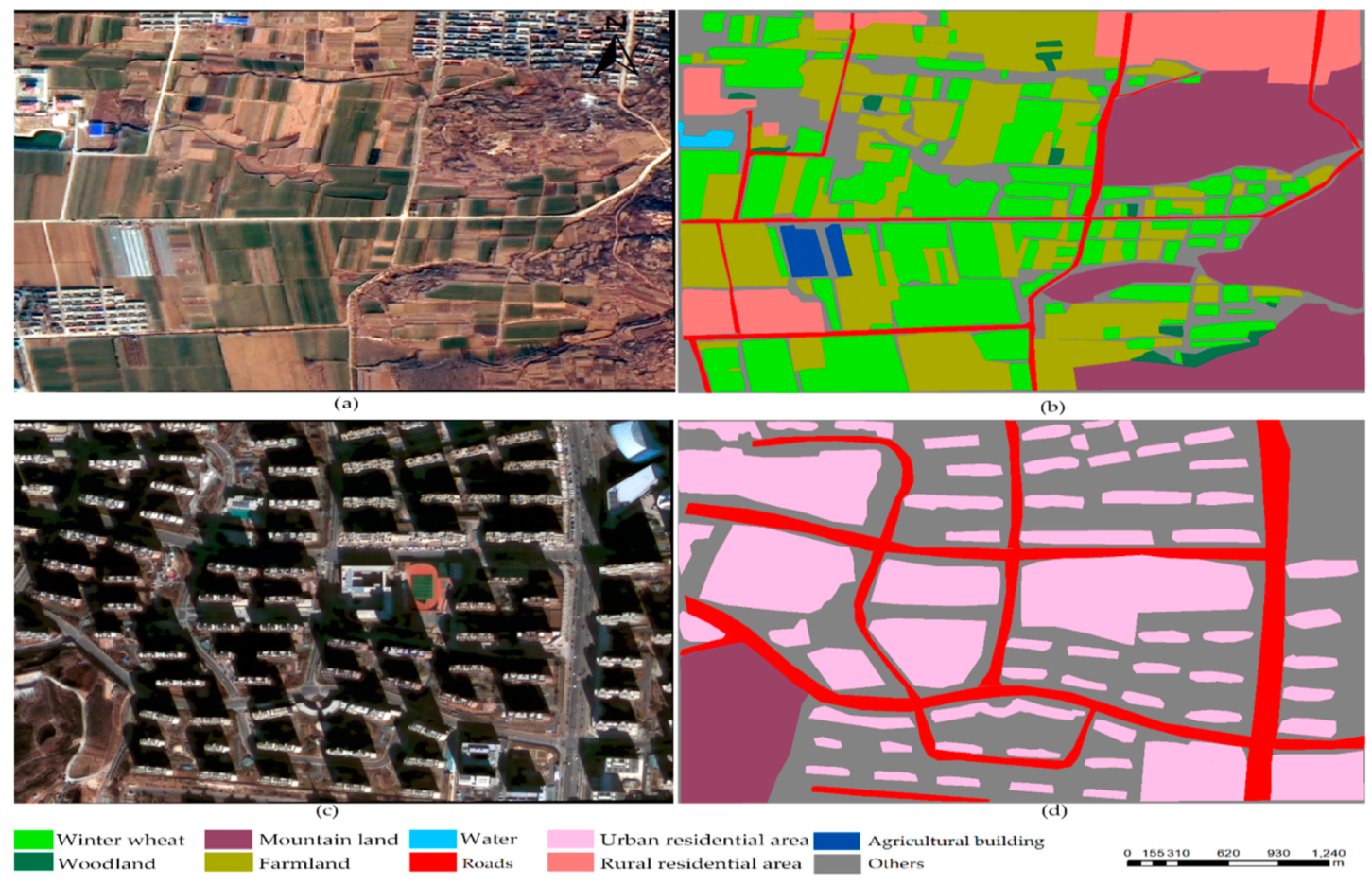
Larger image blocks are advantageous for model training. Considering the hardware used in our research, we cut each pre-processed image into equal-sized image blocks (1000 × 1000 pixels). A total of 920 cloudless image blocks were selected for manual labeling with numbers assigned to the following categories: (1) winter wheat, (2) mountain land, (3) water, (4) urban residential area, (5) agricultural building, (6) woodland, (7) farm land, (8) roads, (9) rural residential area, and (10) others. While selecting the pixel blocks, we used the following principle: each pixel block should contain at least three land-use types, where the area proportion of each land-use type in the selected images was similar to that in the pre-processed images.
We created a label file for each image block, comprising a single-channel image file in which the number of rows and columns was identical to the corresponding image. We used visual interpretation to assign a category number to each pixel and saved it in the corresponding location in the label file. After labeling, the image block and its corresponding label file formed an image–label pair (Figure 2).

3. Methodology

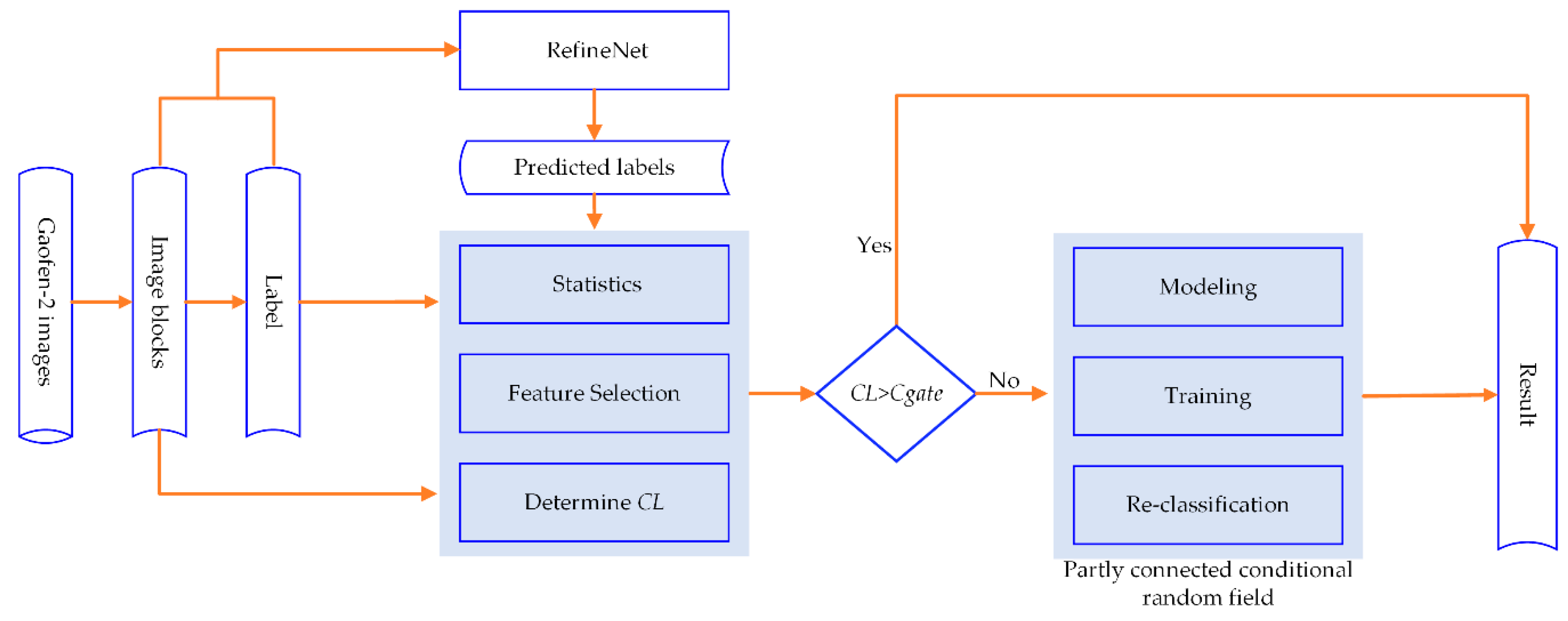
We first modified the original RefineNet model as an initial segmentation model (Section 3.1), and then performed statistical analysis on the initial segmentation results to obtain the prior knowledge (Section 3.2). Based on the obtained knowledge, we constructed the PCCRF model (Section 3.3) and trained the model (Section 3.4). The trained model was then used to refine the initial segmentation results of the CNNs to generate the final results. We designed a set of comparative experiments to evaluate the performance of the proposed method (Section 3.5). Figure 3 summarizes the entire flowchart of the proposed approach.

3.1. Improved RefineNet Model

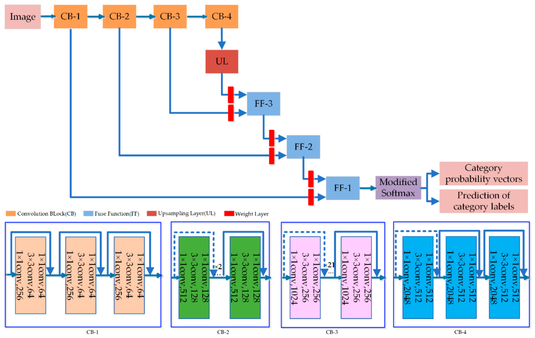
We selected RefineNet as our initial segmentation model. Unlike the FCN, SegNet, DeepLab, and other models, this model uses a multi-path structure that fuses low-level detailed semantic features with high-level rough semantic features, thereby effectively improving the distinguishability of the pixel features. We modified the classic RefineNet model to initially segment remote sensing images; Figure 4 shows the structure of the improved RefineNet model.
Improvements to the RefineNet model were as follows.
First, we replaced the equal weight fusion model used in the classic model with a linear fusion model to fuse detailed low-level semantic features and high-level rough semantic features. The fusion method is as follows:
s = a ×   f + b ×   g ,
where s denotes the fused features, f represents the detailed low-level semantic feature values generated by the convolution block, g denotes the up-sampling feature of the high-level rough semantic features, and a and b are the coefficients of the fusion model. The specific values of a and b must be determined via model training.
Second, we modified the classifier of RefineNet, i.e., Softmax, to simultaneously output the prediction category label and category probability vector, P, for each pixel.
The probability value of a pixel was assigned as the ith category label pi, which was calculated as follows:
p i = e r i 1 m e r j ,
where m is the number of categories, and ri and rj represent the output of the RefineNet encoder, i.e., the product of the pixel’s feature vector and ith feature function, respectively. Based on the definition of pi, P can be defined as follows:
P = ( p 1 , p 2 , , p m ) .
We used the stochastic gradient descent algorithm [79] to train the improved RefineNet model, and used the trained model to segment image blocks to obtain initial segmentation results, including the prediction label image and category probability vectors for each pixel.

3.2. Statistical Analysis of the Initial Segmentation Results

In a previous study [21], we proposed the confidence level, CL, as an indicator to evaluate the credibility degree of the predicted category label of the pixel using the CNN:
C L = p m a x p m a x ,
where pmax represents the maximum value of P and pmax represents the maximum value of P with pmax excluded.
We used Cgate to represent the confidence level threshold. The predicted category label of the pixel was considered credible if CL > Cgate, and not if otherwise. After Cgate was determined, the pixel set I = {1, 2, …, m} was divided into two subsets, as follows:
P C = { i } ,   C L   of   pixel   i C g a t e   of   pixel   i ,
P I C = { i } ,   C L   of   pixel   i < C g a t e   of   pixel   i .
As the classification results of the pixels in the PC were credible, we only needed to post-process the classification results of the pixels in the PIC.
The value of Cgate had a significant impact on the overall accuracy. When Cgate was high, the number of pixels that required post-processing was large, such that there was a significant improvement in the overall classification accuracy. When the value of Cgate was low, the number of pixels that required post-processing was small, but improvements to the overall classification accuracy were not always apparent.
The following steps were used in our study to determine the value of Cgate. First, we used a TIFF file to store the CL while we predicted the category label, category probability vector, and manual-labeled category.
Second, the pixels were divided into two sets based on the artificially-labeled category and predicted category using the following rules:
P R = { i } ,   mannul   category   label   of   pixel   i = Predicted   category   label   of   i ,
P W = { i } , mannul   category   label   of   pixel   i Predicted   catagory   label   of   i .
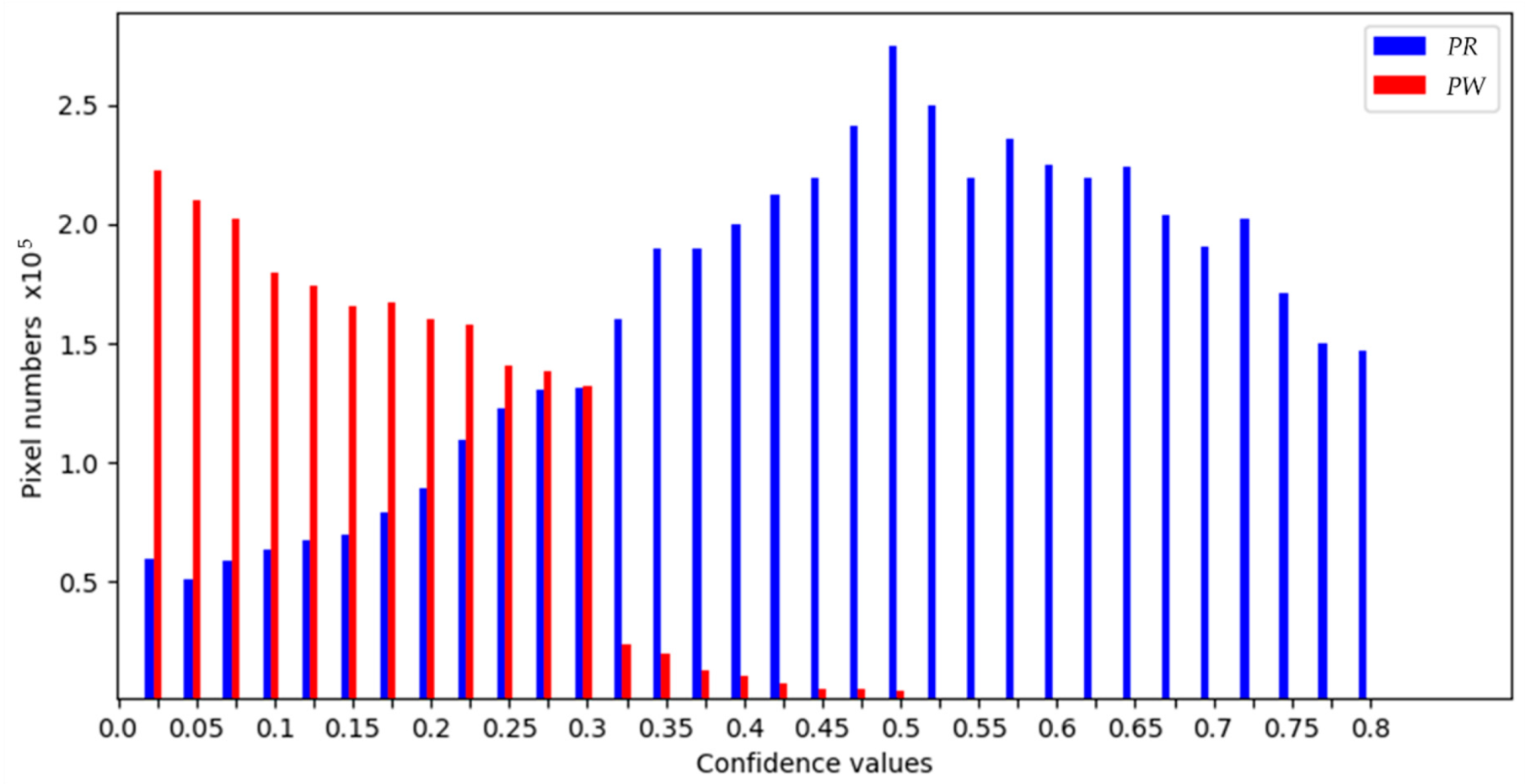
Third, a histogram was produced for PR and PW using the CL as the x-axis and the number of pixels corresponding to a certain CL value as the y-axis. Figure 5 provides an example of a histogram, which was used to determine the value of Cgate. In general, the principle is that when CL is greater than Cgate, the number of misclassified pixels should be as small as possible.

3.3. The PCCRF Model

3.3.1. Description of the Modeling Scheme

According to the obtained prior knowledge, in the classification results generated by the CNN, the results for the pixels located inside the object are credible, but the credibility of the pixels located at the edge of the object is low. Furthermore, only low-credibility classification results require post-processing.
Based on previous studies [51,52,53,58,59], approximately 80% of the pixel-by-pixel classification results generated by CNN models are credible. Therefore, only approximately 20% of the pixel classification results require post-processing. This strategy can significantly reduce the number of calculations, thereby improving the efficiency and performance of the model. This is in reference to our use of term “partly connected.”
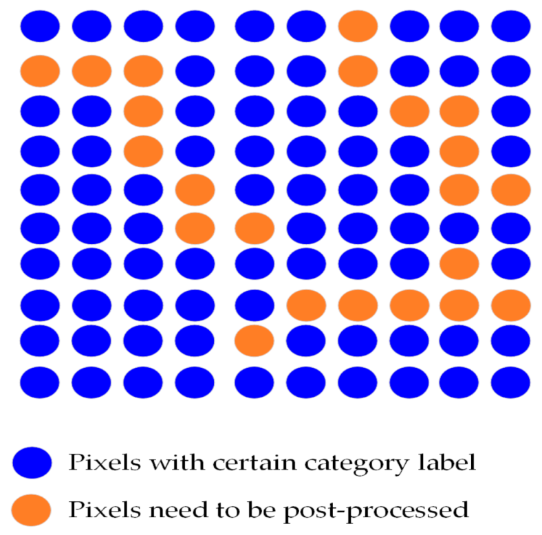
Based on the abovementioned analysis, we consider the following case: on a given image, when the category labels of certain pixels have been determined by the CNN, how the category labels of the remaining pixels are to be determined needs to be clarified (Figure 6).
We can observe that the main difference between the PCCRF and FCCRF is that the former can take full advantage of the fact that certain pixels have already been assigned certain category labels.
In the PCCRF, we used the category probability vectors generated by the CNN to build a unary potential energy similar to the FCCRF by using the relationship between pixel pairs to build a pairwise potential energy. Considering that there are numerous mixed pixels on the remote sensing image, we must select appropriate features to form a feature vector for the pixels (Section 3.3.2), and then use these vectors to define the pairwise potential energy (Section 3.3.3). Based on this, we can provide the definition of a PCCRF (Section 3.3.4).

3.3.2. Features Selection

Based on prior knowledge, the inner and edge pixels of the winter wheat planting areas are extremely similar in terms of color and texture. Considering that the near-infrared band (NIR) can better distinguish between crops and non-crops, we selected the red, blue, green, and NIR bands, along with the NDVI, contrast (CON), uniformity (UNI), inverse difference (INV), and entropy (ENT), to construct the feature vectors for the pixels. The NDVI was calculated following the methods reported in Ma et al. [17]:
N D V I = N I R R e d N I R + R e d .
Here, CON, UNI, INV, and ENT were extracted using the methods proposed by Yang and Yang [27], based on the GLCM:
C O N = n = 0 q 1 n 2 { i = 1 q j = 1 q g ( i , j ) }   where   | i j | = n ,
U N I = i = 1 q j = 1 q ( g ( i , j ) ) 2 ,
I N V = i = 1 q j = 1 q g ( i , j ) 1 + ( i j ) 2 ,
E N T = i = 1 q j = 1 q ( g ( i , j ) log { g ( i , j ) } ,
where q is the gray level and g(i,j) is an element of the GLCM.
The feature vector f of each pixel comprises nine elements, structured as follows:
f = ( r e d , g r e e n , b l u e , N I R , N D V I , U N I , C O N , E N T , I N V ) .

3.3.3. Definition of the Pairwise Potential Energy

Based on the Gaussian kernel function, we define the potential energy of a pixel pair, τ ( x i , x j ) , as:
τ ( x i , x j ) = μ ( x i , x j ) ( ω ( 1 ) e x p ( | | f i f j | | 2 2 θ α 2 | | I i I j | | 2 2 θ β 2 ) + ω ( 1 ) e x p ( | | f i f j | | 2 2 θ γ 2 ) ) ,
where i and j each represent a single pixel of image I, xi is the predicted category label of pixel i by the CNN, xj represents the predicted category label of pixel j by the CNN, xi and xj are elements of category label set L = {l1, l2, …, ln}, f i , f j represent the feature vector of the pixel, as discussed in Section 3.3.2, | | I i I j | | is the Manhattan distance between i and j, | | f i f j | | is the Euclidean distance between i and j, and μ( x i , x j ) is the label comparison function. When x i and x j are identical, the value was set to 0; otherwise, it is set to 1. Here, ω ( 1 ) ,   ω ( 2 ) , θ α , θ β , and θ γ are determined through training the PCCRF.
Based on the definition of τ i j , we can define the sum of the pairwise potential energy of xi, τ ( x i ) , as:
τ ( x i ) = j I   τ ( x i , x j ) .
The total pairwise potential energy associated with i is defined as follows:
τ ( i ) = x i L τ ( x i ) .
Considering that the unary potential energy is an element of the category probability vector, the value range is [0, 1], and therefore, we used τ ( i ) to normalize τ ( x i ) :
n τ ( x i ) = τ ( x i ) τ ( i ) .
We used n τ ( x i ) to build the PCCRF.

3.3.4. Definition of PCCRF

As discussed in Section 3.2, I is the set of pixels and PC and PIC are the subsets of I. As the classification results of the pixels in PC were credible, we only needed to optimize the classification results of the pixels in PIC. Based on the above-mentioned analysis, we only used such pixel pairs to build the PCCRF, where at least one pixel in the pixel-pair belonged to PIC.
Let i be a pixel in PIC and j be a pixel in I. Therefore, x = {x1, x2, …, xm} represents a label set assignment of PIC. Then, θ represents the model parameter set of ω ( 1 ) , ω ( 2 ) , θ α , θ β , and θ γ . We define the Gibbs energy of x as follows:
E ( x | P I C , θ ) = i P I C ( φ ( x i ) + ( 1 ) n τ ( x i ) ) ,
where φ ( x i ) represents the unary potential energy of x i , φ ( x i ) is an element of the category probability vector of pixel i generated by the CNN, is the weight value for the unary potential energy, and ( 1 ) is the weight value for the pairwise potential energy. Here, is determined while training the PCCRF.
Based on the above analysis, we define the PCCRF as follows:
P ( X = x | P I C , θ ) = E ( x | P I C , θ ) y X E ( y | P I C , θ ) ,
where X represents the set of all possible label set assignments of the PIC and y represents a label set assignment of the PIC.
By minimizing the above CRF energy, E(x), we can assign an optimal set of labels to the PIC.
In the PCCRF, φ ( x i ) provides the information from a large receptive field to predict the category label for a pixel, while n τ ( x i ) provides additional information from a small receptive field to optimize the category label.
The PCCRF takes full advantage of prior information. When the predicted category of the pixel using the CNN is credible, the category label can be determined using only the information from a large receptive field. Otherwise, it uses additional information to optimize the category label.

3.4. PCCRF Training

We defined the objective function of the PCCRF based on the cross-entropy of the samples as follows:
H ( p , q ) = q = 1 t q i log ( p i ) ,
where p is the predicted category probability distribution (CPD) output by the PCCRF, q is the actual CPD, t is the number of category labels, and i is the index of an element in the CPD. Based on this, the loss function of the PCCRF model was defined as follows:
Loss = 1 Total t s i = 1 t q i log ( p i ) ,
where Total is the number of samples used in the training stage. We then used the stochastic gradient descent to train the model via the following steps:
  • Pretrained the RefineNet;
  • Constructed the PCCRF training dataset using the training prediction results generated by the trained RefineNet;
  • Performed statistical analysis on the training dataset and determined the value of Cgate;
  • Initialized the parameters of the PCCRF model; and
  • Calculated the parameters of the PCCRF using the method proposed in Zheng et al. [55].

3.5. Experimental Setup

We conducted comparison experiments based on the RefineNet (which combines low-level and high-level features) and SegNet (which only uses high-level semantic features) using three levels of configuration for each experiment: the original model, classic CRF post-processing, and PCCRF post-processing (Table 1).
We applied data augmentation techniques on the training dataset, such as horizontal flip, color adjustment, and vertical flip steps. The color adjustment factors included brightness, hue, saturation, and contrast. Each image in the training dataset was processed 10 times. All images created using the data augmentation techniques were only used for training the CNNs.
We used cross-validation techniques in the comparative experiments. Each CNN model was trained over five rounds. In each round, 200 images were selected as test images and the other images were used as training images to guarantee that each image was used at least once as a test image.
Table 2 lists the hyper-parameter setup used to train the proposed RefineNet-PPCRF. In the comparison experiments, the hyper-parameters were also applied to the comparison model.

4. Results and Evaluation

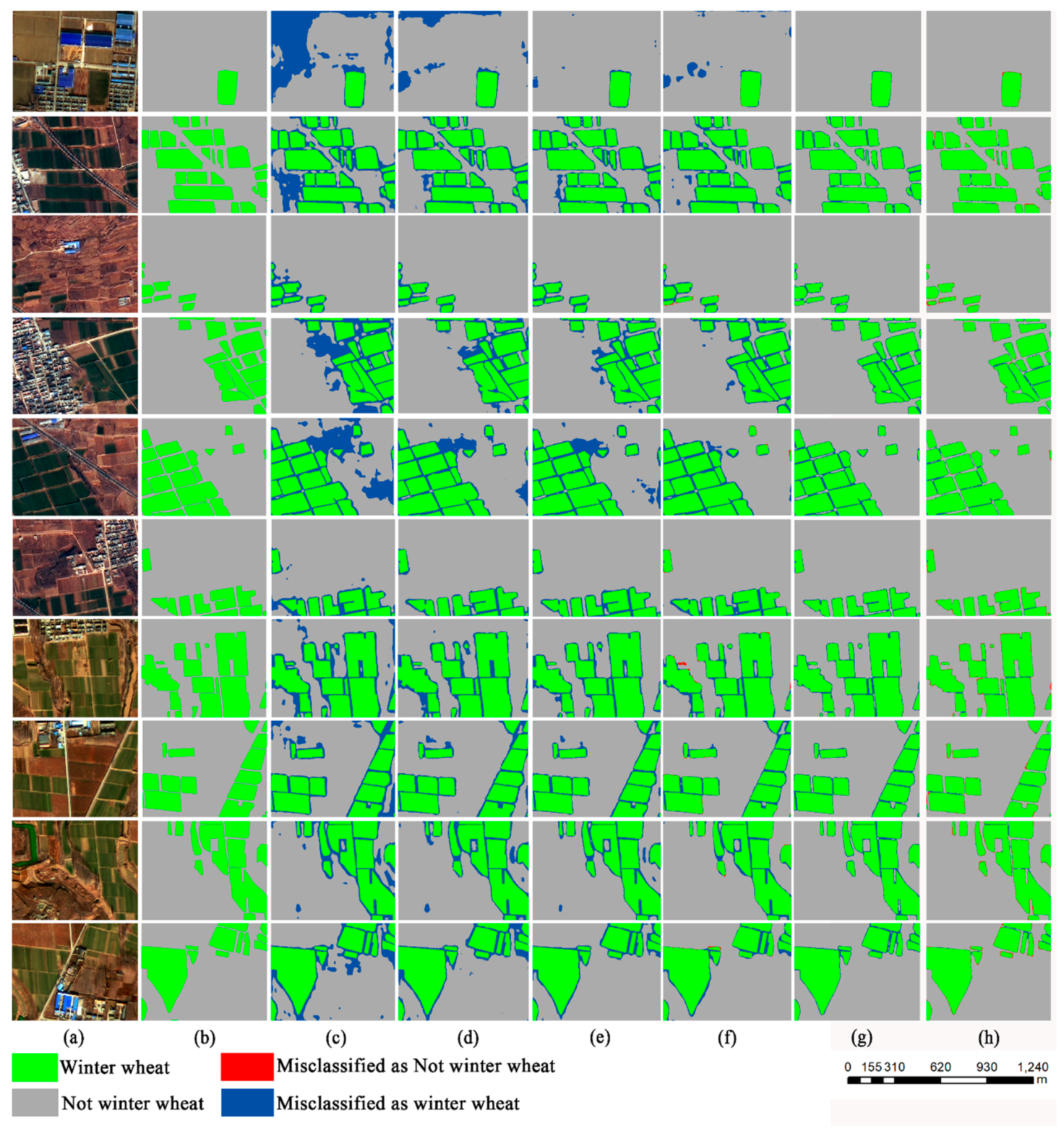
Figure 7 presents 10 randomly selected image blocks and their corresponding results using the six comparison methods.
Although there were certain misclassified pixels in the inner regions of the winter wheat planting area in the SegNet results, the overall classification accuracy of each comparison method in the inner regions of the winter wheat planting area was satisfactory. The difference between the result of the six comparison modes at the edge was observable. In the SegNet results, the edges of the winter wheat fields were rough, and therefore, the RefineNet results were superior to those of the SegNet, thereby demonstrating the importance of using fused features over high-level features. Both the CRF and PCCRF post-processing methods produced superior results, thus demonstrating the importance of post-processing procedures. The SegNet-PCCRF was superior to SegNet-CRF, while the RefineNet-PCCRF was superior to the RefineNet-CRF; this demonstrated that the PCCRF was more suitable as a post-processing method. Comparing the SegNet-PCCRF and RefineNet-CRF, the performance of the RefineNet-CRF was superior, thereby confirming that the initial segmentation method was also a an extremely significant factor in determining the final result.
We used four popular criteria, named accuracy, precision, recall, and F1-score [80] to evaluate the performance of the proposed model. They were calculated using the confusion matrix.
Accuracy is the ratio of the number of correctly classified samples to the total number of samples, calculated as:
Accuracy = i = 1 m c i i i = 1 m j = 1 m c i j   ,
where c i i denotes the number of correctly classified samples, and c i j is the number of samples of class i misidentified as class j. Precision denotes the average proportion of pixels correctly classified into one class from the total retrieved pixels, calculated as:
Precision = 1 2 i c i i / j c i j   .
Recall represents the average proportion of pixels that are correctly classified in relation to the actual total pixels of a given class, calculated as:
Recall = 1 2 i c i i / i c i j   .
F1-score represents the harmonic mean of precision and recall, calculated as:
F 1 = 2 · Precision × Recall Precision + Recall   .
We evaluated the results using the accuracy, precision, recall, and F1-score. The RefineNet-PCCRF scored highest among all models using all metrics (Table 3).
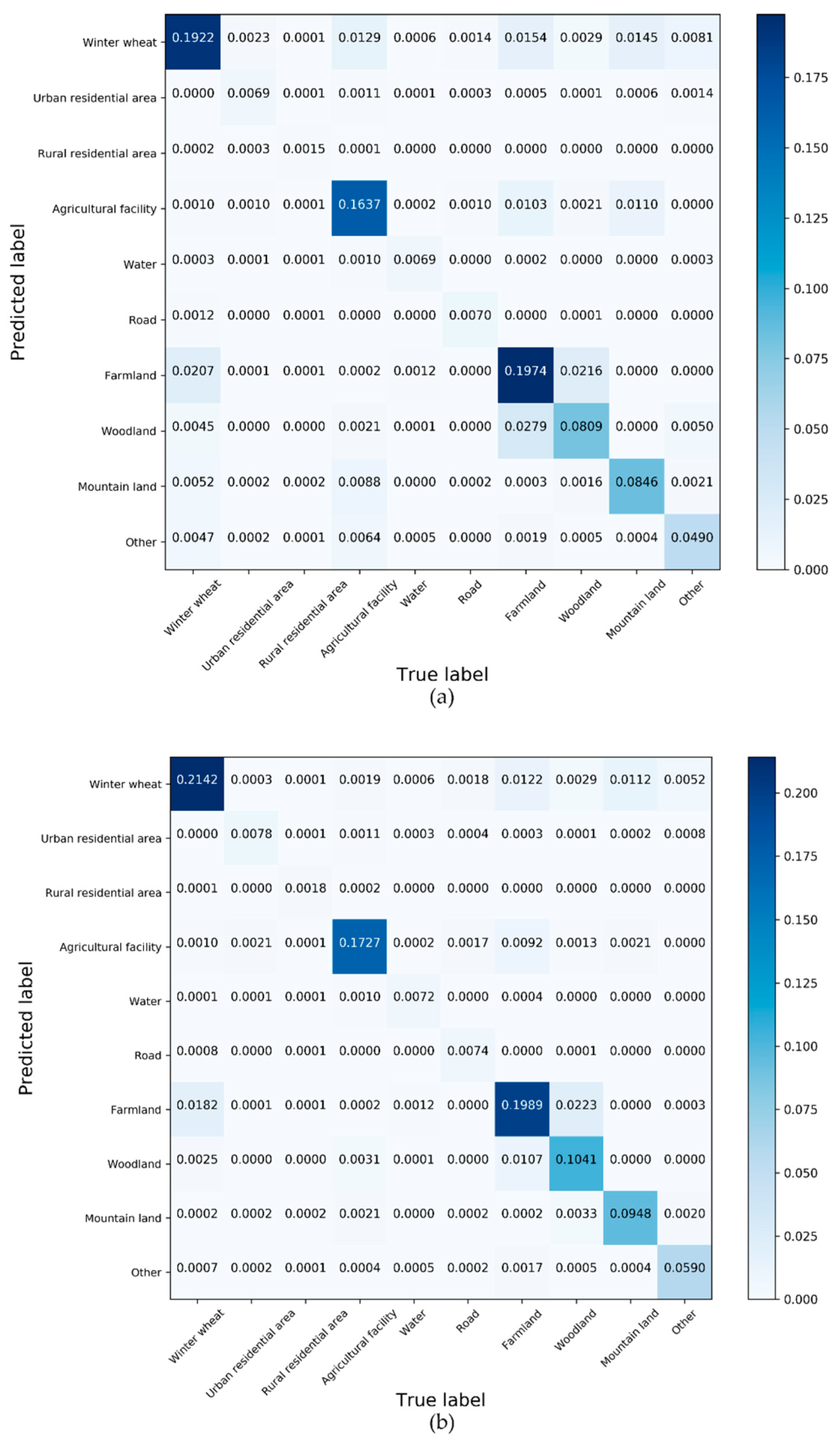
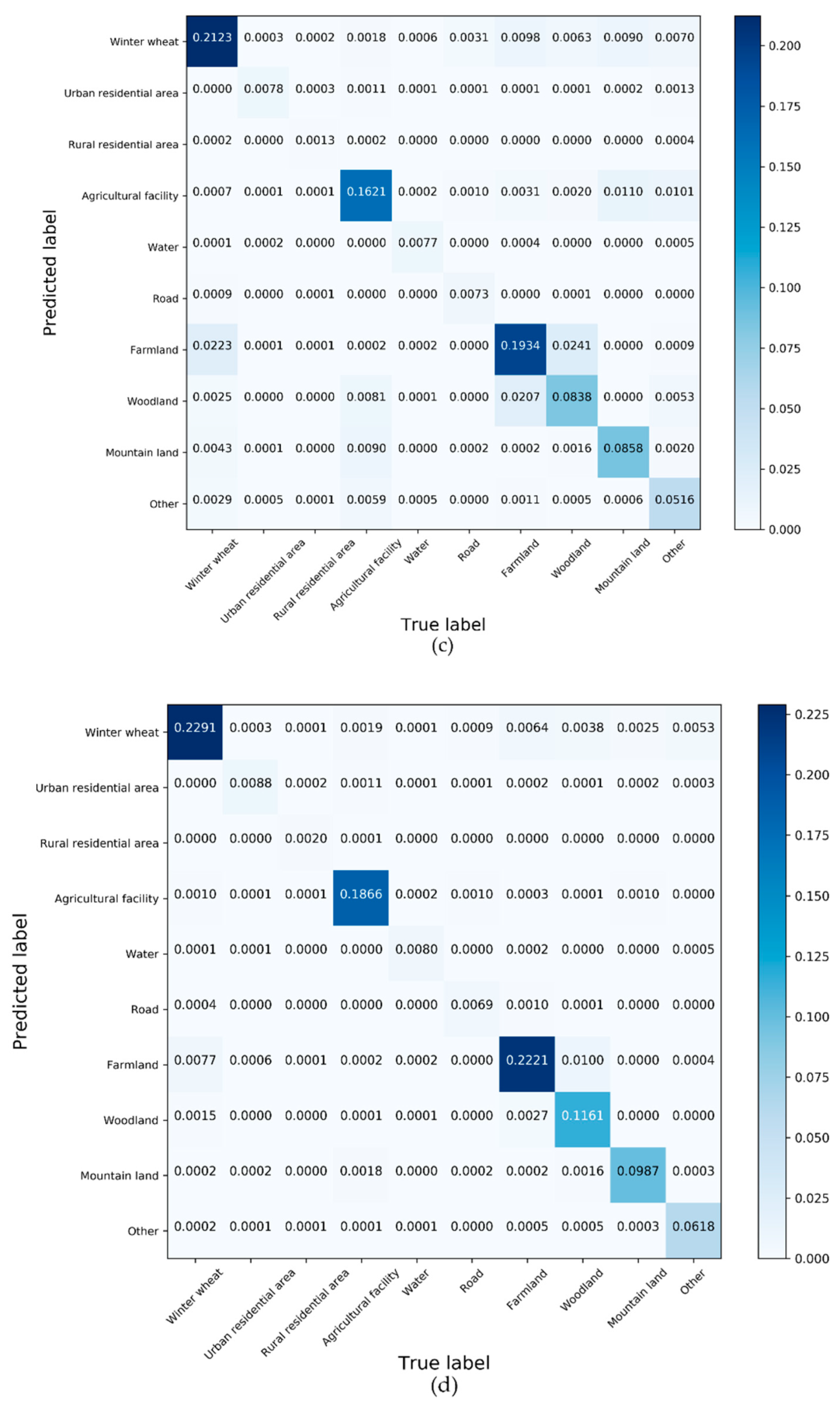
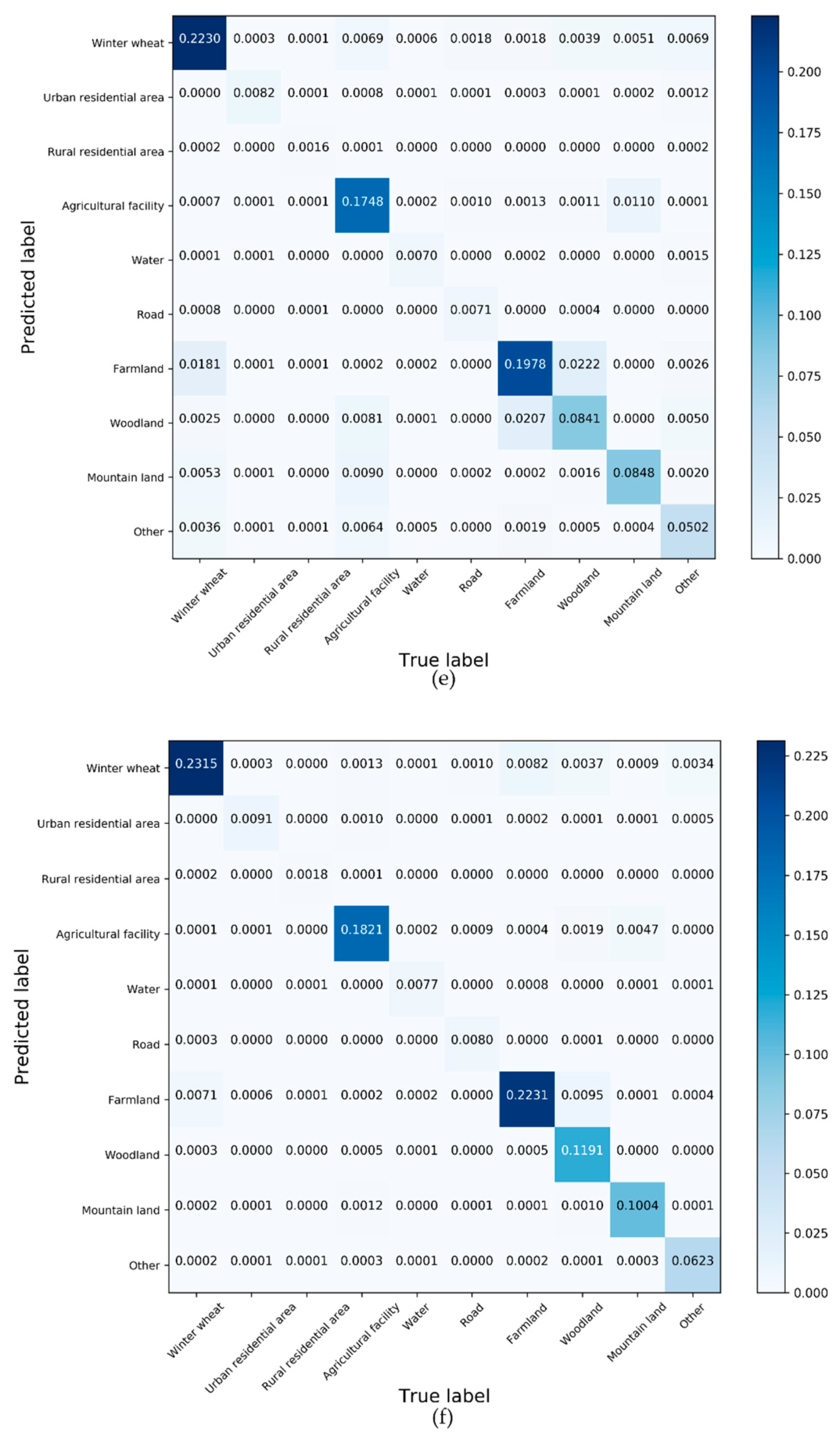
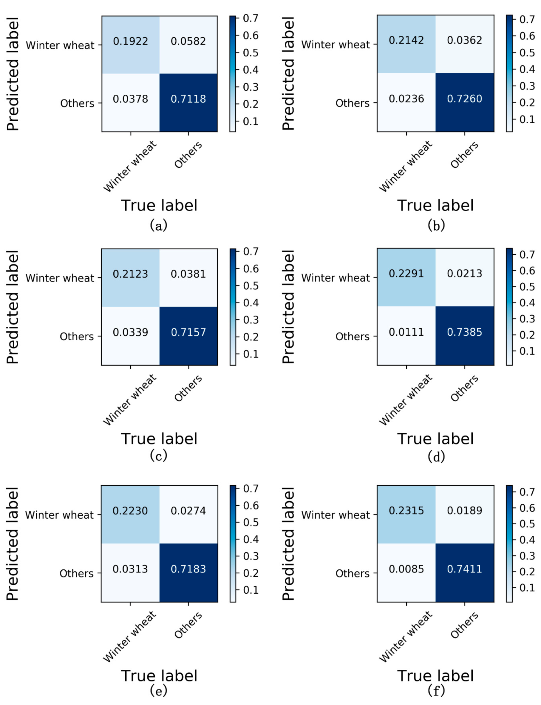
The confusion matrices for all categories (Figure 8) and The confusion matrices for winter wheat and others (Figure 9) for each models demonstrating that the RefineNet-PCCRF achieved the best segmentation results.
In the confusion matrices of the six models, there was nearly no confusion between the winter wheat and urban areas. This could be attributed to the difference in the characteristics of the two land-use types. However, the confusion between winter wheat and farmland was serious. This was because most winter wheat regions that were misclassified as farmlands had poor growing conditions. In these areas, their characteristics were similar to those of farmlands in winter, which led to a greater probability of misclassification. There was also a certain degree of confusion in the winter wheat and woodland areas. This was because certain trees were still green in winter, similar to the characteristics in the regions of winter wheat. However, in this case, due to the use of both texture and high-level semantic information, the degree of confusion was significantly lower than that of farmland. This also explained the advantage of post-processing from another aspect, as it led to the introduction of new information, which could effectively improve the accuracy of the classification results.
Table 4 lists the average time required for each method to complete the testing of a single image. The proposed RefineNET-PPCRF method required approximately 3% more time but improved the accuracy by 5%–8%. The time consumed by the CRF was higher than that using the proposed PCCRF method because the CRF had to calculate the distances between all pixel–pixel pairs for a single image, while the proposed PCCRF method calculated the distances for only a small number of pixel–pixel pairs. The number of pixel–pixel pairs calculated in the SegNet-PCCRF was only approximately 30% of that of the SegNet-CRF. The number of pixel–pixel pairs calculated in the RefineNet-PCCRF is only approximately 20% of that in the RefineNet-CRF.

5. Discussion

5.1. PCCRF Necessity

The CNN models typically use multiple convolutional layers to obtain high-level semantic features, which then assign the features to each pixel in the receptive field through a deconvolution operation. When the operation is performed at the edges of the object, since there may be two or more types of pixels in the sensory field, this can cause differences in the feature values of edges and inner pixels, resulting in a higher classification error at object edges (Figure 7).
The structural characteristics of the convolutional neural network indicate that there will be inevitable misclassification of pixels at the edges. This problem can only be improved using post-processing methods or improving the structure of the convolutional neural network.
At present, numerous post-processing methods have been proposed, but most of these methods fail to make full use of the results provided by convolutional neural networks. The PCCRF proposed in this study comprehensively uses the advantages of the CRF and prior knowledge provided by the CNN, which is a more effective post-processing method.

5.2. Comparison between PCCRF and FCCRF

PCCRF has three clear advantages over FCCRF. First, it has a clearer model structure. In PCCRF, a category probability vector is used to express the calculation result, and each component represents the probability that the pixel to be processed is classified into a certain category. The class probability vector of a pixel is divided into two levels for calculation: (1) a pixel-level class probability vector that represents the class probability distribution calculated on the basis of the characteristics of the pixel itself and (2) a class-level class probability vector that represents a class probability distribution calculated on the basis of the class of pixels around the pixel to be classified. The scale factor expresses the fusion of two types of information in which the two messages involved in the fusion have the same meaning. In contrast, in FCCRF, each component of the first level vector is a class feature value calculated on the basis of the characteristics of the pixel itself, whereas each component of the second-level vector is a category feature value calculated on the basis of the category information of the pixel to be processed and the surrounding pixels. The two feature values with different properties are added together to produce the class feature value of the pixel. The meaning of the eigenvalues obtained using this processing method is not clear enough.
Second, FCCRF does not introduce any prior knowledge, and all pixel-pairs need to be calculated, which leads to overcalculation. Hence, there is a need to solve model parameters through finding approximate values. In contrast, PCCRF introduces prior knowledge and only processes pixels with low classification reliability, effectively reducing the number of calculations and directly solving the model through methods such as the stochastic gradient descent algorithm.
Third, PCCRF uses color, texture, and low-level semantics to form feature vectors, which is more in line with the characteristics of remote sensing data. FCCRF obtains good results using only color features because the camera image resolution is usually very high and the detailed information is very rich. The color of the pixels often differs greatly where two objects are adjacent. However, in remote sensing imagery, a large number of mixed pixels means that the differences in the pixel color of two objects are often much smaller, and hence, the additional information used by PCCRF improves its classification performance.

5.3. Cgate Effect

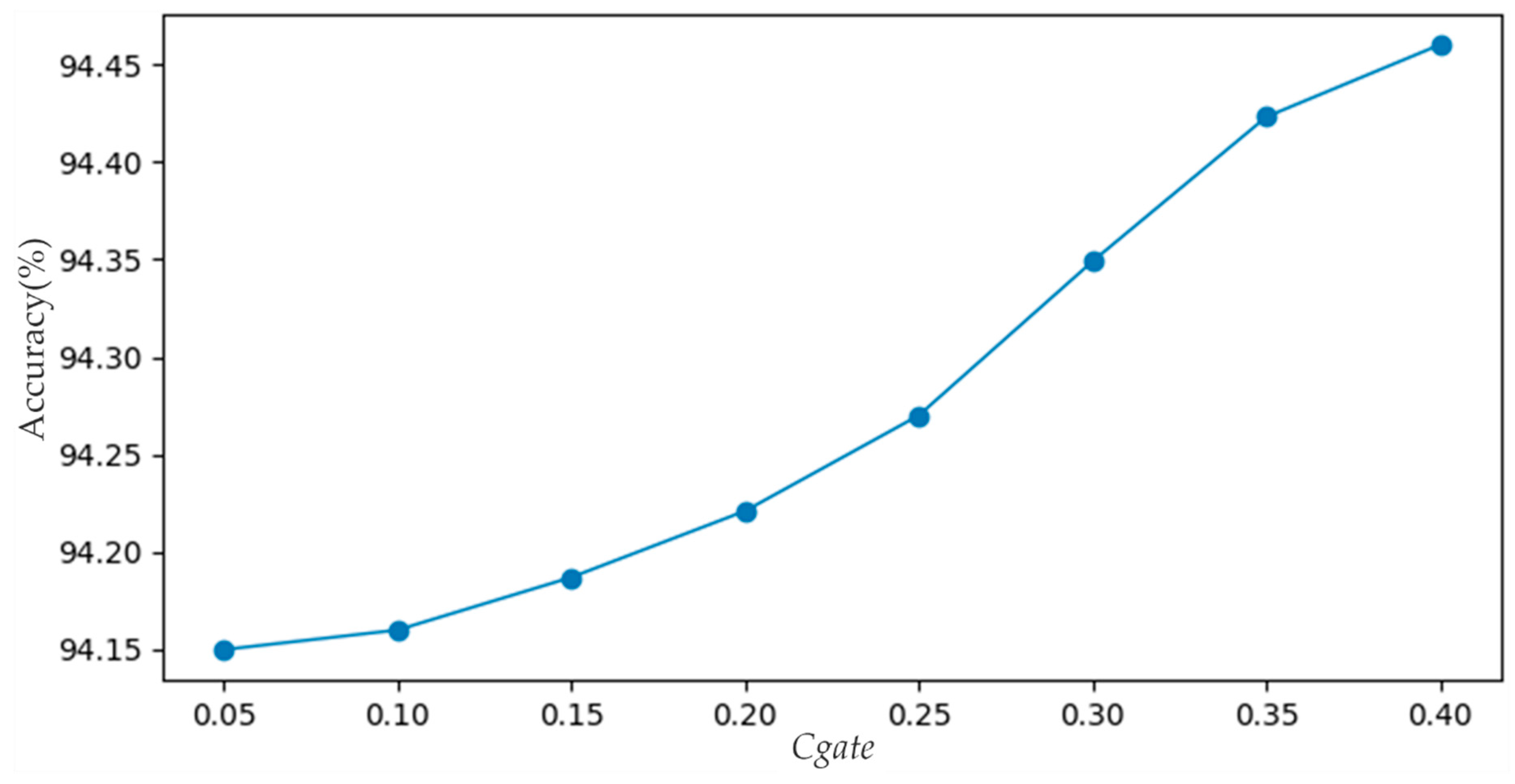
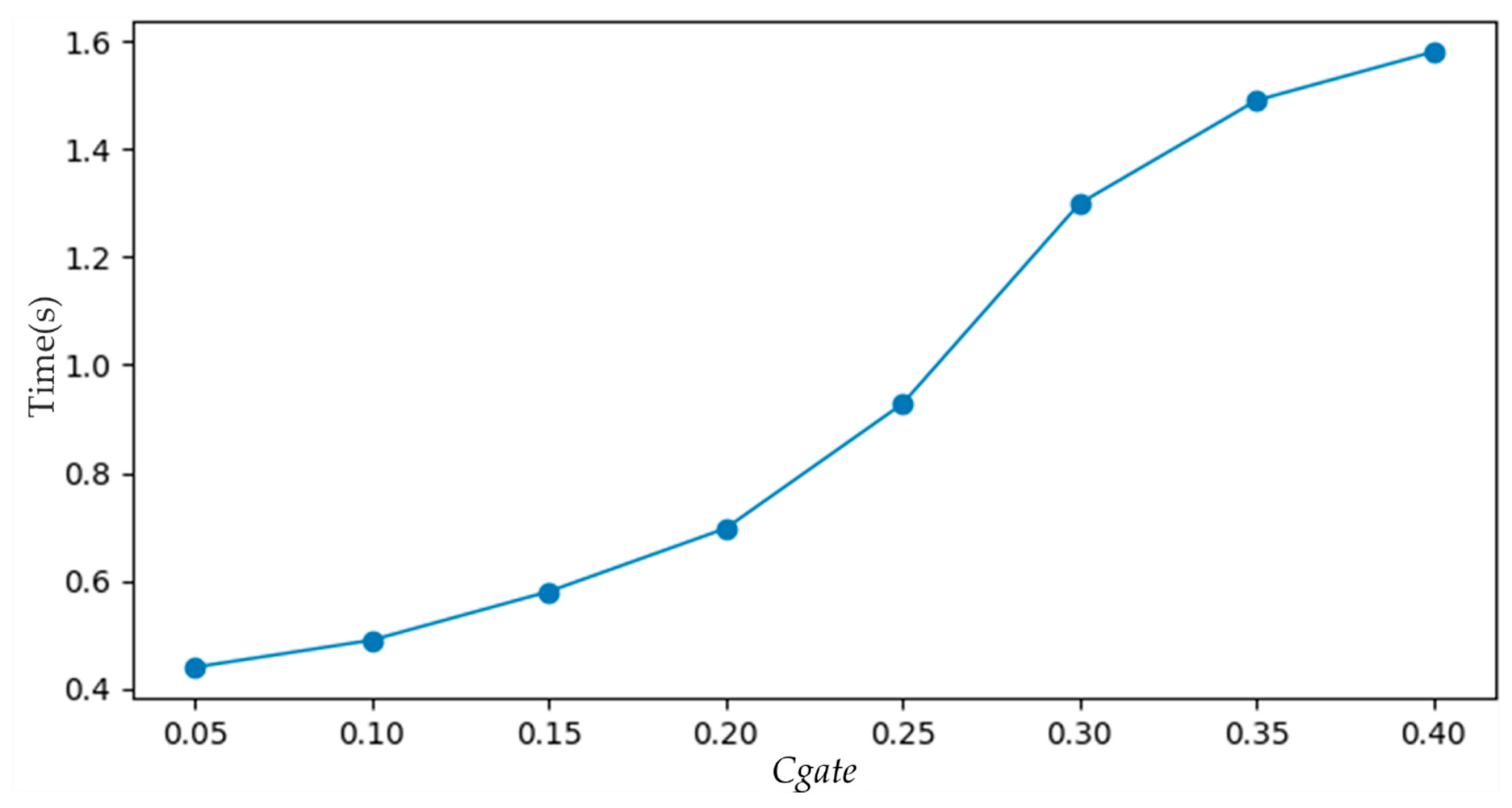
Given the overall importance of the Cgate parameter in the RefineNet-PCCRF, we held other parameters steady and calculated the relationships among the Cgate, accuracy (Figure 10), and consumed time (Figure 11).
Higher Cgate values improved the accuracy because pixels were filtered with a higher level of confidence. Post-processing resulted in the reclassification of the initially misclassified pixels, thus improving the accuracy of the overall result. Therefore, when selecting the Cgate value, we must consider the classification ability of the initial segmentation model. In addition, selecting a model with a stronger classification ability for preliminary segmentation can significantly improve the performance of the results obtained from the PCCRF model. Higher Cgate values also increased the consumed time; this indicated that a further reduction in the number of pixels involved in modeling, i.e., using more prior knowledge, is the key to further improving the calculation efficiency of both the PCCRF and classic CRF models.

5.4. Comparison between PP-CNN and RefineNet-PPCRF

To obtain high-quality spatial distribution information of winter wheat, we used an improved Euclidean distance to establish PP-CNN as a post-processing method [81]. According to the improved Euclidean distance of the feature vector between a pixel being classified and the determined winter wheat pixel, it can be determined whether the pixel being classified is displaying winter wheat. Unlike the PP-CNN, the proposed PCCRF was established on the basis of the CRF. Due to the advantage of the CRF using global distribution characteristics, the PP-CRF can more accurately determine the category label of the edge of the winter wheat planting area.
In general, the PP-CNN can be used in cases where the feature differences are stable between the mixed pixels on the edge of the winter wheat planting area and the inner pixels of the same area. When the difference is unbalanced, the distance threshold bias is large, which increases the probability of pixel classification errors during post-processing. The PCCRF fully considers the spatial correlation between pixel categories, hence yielding a strong global balance ability. Therefore, this method can better handle situations where the edge pixels are significantly different from the inner pixels, thereby effectively reducing the impact of large differences in crop growth.

6. Conclusions

CNNs can significantly improve the overall accuracy of remote sensing image segmentation results. However, in the segmentation results, there are certain misclassified pixels in the adjacent land-use types. This study used the advantages of the CRF model that can describe the spatial correlation between pixel categories, introduced a variety of prior knowledge, and proposed a PCCRF model. The proposed PCCRF model can be used to post-process the results of the CNN to better solve the problem of rough edges in the results extracted using only the CNN.
The main contributions of this study are as follows: (1) Pre-processing (such as statistical analysis of the CNN segmentation results) allows for the use of post-processing and modeling of prior knowledge, such that only those pixels with a lower confidence are processed, thus significantly reducing calculation time. As the RefineNet has high segmentation accuracy, this post-processing only requires the use of 20% of all the pixels. (2) According to the characteristics of the winter wheat planting area on the remote sensing image, the PCCRF uses original channel values, texture features, and low-level semantic features to compose the feature vector and construct the pairwise potential energy. This feature vector better matches the characteristics of the remote sensing imagery. At the same time, after normalizing the pairwise potential energy, the data range is identical to that of the unary potential energy. This aspect is more reasonable than that of the FCCRF. (3) The PCCRF uses a linear model to fuse the unary energy and pairwise energy such that the parameters of the linear mode are determined while training the PCCRF. This strategy is more reasonable than the fixed weight value strategy adopted by the FCCRF. Due to the ability to describe the globe spatial correlation between pixel categories of the CRF, the RefineNet-PCCRF can efficiently improve the classification accuracy of edge pixels in a winter wheat planting area.
As the prior knowledge required by the PCCRF can only be obtained via statistical analysis of the CNN segmentation results, the PCCRF and CNN must be used separately to generate improved extraction results, which is the major limitation of our method. In future studies, we intend to use hyperparameters and other means to express prior knowledge, convert the PCCRF into convolution operations, and construct a complete end-to-end training model.

Author Contributions

Conceptualization: C.Z. and Z.X.; methodology: C.Z. and Z.X.; software: S.W., H.Y., and Z.Z.; validation: Y.W.; formal analysis: C.Z., Z.X., and S.W.; investigation: H.Y., and Z.Z.; resources, S.G.; data curation, S.G. and Y.W.; writing—original draft preparation, C.Z., Z.X., and S.W; writing—review and editing: C.Z.; visualization: S.G.; supervision: C.Z.; project administration: C.Z. and S.G; funding acquisition: C.Z. All authors have read and agreed to the published version of the manuscript.

Funding

This research was funded by the National Key R&D Program of China, grant numbers 2017YFA0603004 and 2017YFD0301004; the Science Foundation of Shandong, grant number ZR2017MD018; the Key Research and Development Program of Ningxia, grant number 2019BEH03008; the Open Research Project of the Key Laboratory for Meteorological Disaster Monitoring, Early Warning and Risk Management of Characteristic Agriculture in Arid Regions, grant numbers CAMF-201701 and CAMF-201803; and the arid meteorological science research fund project by the Key Open Laboratory of Arid Climate Change and Disaster Reduction of China Meteorological Administration (CMA), grant number IAM201801. The Article Processing Charges (APC) was funded by ZR2017MD018.

Acknowledgments

The authors would like to thank Zhongshan Mu and Tianyu Zhao for data provision and participating in field investigation.

Conflicts of Interest

The authors declare no conflict of interest.

References

  1. Chen, X.-Y.; Lin, Y.; Zhang, M.; Yu, L.; Li, H.-C.; Bai, Y.-Q. Assessment of the cropland classifications in four global land cover datasets: A case study of Shaanxi Province, China. J. Integr. Agric. 2017, 16, 298–311. [Google Scholar] [CrossRef] [Green Version]
  2. Ma, L.; Gu, X.; Xu, X.; Huang, W.; Jia, J.J. Remote sensing measurement of corn planting area based on field-data. Trans. Chin. Soc. Agric. Eng. 2009, 25, 147–151. (In Chinese) [Google Scholar] [CrossRef]
  3. Nabil, M.; Zhang, M.; Bofana, J.; Wu, B.; Stein, A.; Dong, T.; Zeng, H.; Shang, J. Assessing factors impacting the spatial discrepancy of remote sensing based cropland products: A case study in Africa. Int. J. Appl. Earth Obs. 2020, 85, 102010. [Google Scholar] [CrossRef]
  4. Song, Q.; Hu, Q.; Zhou, Q.; Hovis, C.; Xiang, M.; Tang, H.; Wu, W. In-Season Crop Mapping with GF-1/WFV Data by Combining Object-Based Image Analysis and Random Forest. Remote Sens. 2017, 9, 1184. [Google Scholar] [CrossRef] [Green Version]
  5. Atzberger, C.; Rembold, F. Mapping the Spatial Distribution of Winter Crops at Sub-Pixel Level Using AVHRR NDVI Time Series and Neural Nets. Remote Sens. 2013, 5, 1335–1354. [Google Scholar] [CrossRef] [Green Version]
  6. Zhang, J.; Feng, L.; Yao, F. Improved maize cultivated area estimation over a large scale combining MODIS–EVI time series data and crop phenological information. ISPRS J. Photogramm. Rem. Sens. 2014, 94, 102–113. [Google Scholar] [CrossRef]
  7. Jiang, T.; Liu, X.; Wu, L. Method for mapping rice fields in complex landscape areas based on pre-trained convolutional neural network from HJ-1 A/B data. ISPRS Int. J. Geo-Inf. 2018, 7, 418. [Google Scholar] [CrossRef] [Green Version]
  8. Wang, L.; Jia, L.; Yao, B.; Ji, F.; Yang, F. Area change monitoring of winter wheat based on relationship analysis of GF-1 NDVI among different years. Trans. Chin. Soc. Agric. Eng. 2018, 34, 184–191. (In Chinese) [Google Scholar] [CrossRef]
  9. Wang, D.; Fang, S.; Yang, Z.; Wang, L.; Tang, W.; Li, Y.; Tong, C. A regional mapping method for oilseed rape based on HSV transformation and spectral features. ISPRS Int. J. Geo-Inf. 2018, 7, 224. [Google Scholar] [CrossRef] [Green Version]
  10. Georgi, C.; Spengler, D.; Itzerott, S.; Kleinschmit, B. Automatic delineation algorithm for site-specific management zones based on satellite remote sensingdata. Precis. Agric. 2018, 19, 684–707. [Google Scholar] [CrossRef] [Green Version]
  11. Mhangara, P.; Odindi, J. Potential of texture-based classification in urban landscapes using multispectral aerial photos. S. Afr. J. Sci. 2013, 109, 1–8. [Google Scholar] [CrossRef] [Green Version]
  12. Wang, F.; Kerekes, J.P.; Xu, Z.Y.; Wang, Y.D. Residential roof condition assessment system using deep learning. J. Appl. Remote Sens. 2018, 12, 016040. [Google Scholar] [CrossRef] [Green Version]
  13. Du, S.; Du, S.; Liu, B.; Zhang, X. Context-Enabled Extraction of Large-Scale Urban Functional Zones from Very-High-Resolution Images: A Multiscale Segmentation Approach. Remote Sens. 2019, 11, 1902. [Google Scholar] [CrossRef] [Green Version]
  14. Kavzoglu, T.; Erdemir, M.Y.; Tonbul, H. Classification of semiurban landscapes from very high-resolution satellite images using a regionalized multiscale segmentation approach. J. Appl. Rem. Sens. 2017, 11, 035016. [Google Scholar] [CrossRef]
  15. Pan, X.; Zhao, J. A central-point-enhanced convolutional neural network for high-resolution remote-sensing image classification. Int. J. Remote Sens. 2017, 38, 6554–6581. [Google Scholar] [CrossRef]
  16. Ji, S.; Zhang, C.; Xu, A.; Shi, Y.; Duan, Y. 3D Convolutional Neural Networks for crop classification with multi-temporal remote sensing images. Remote Sens. 2018, 10, 75. [Google Scholar] [CrossRef] [Green Version]
  17. Ma, Y.; Fang, S.H.; Peng, Y.; Gong, Y.; Wang, D. Remote estimation of biomass in winter oilseed rape (Brassica napus L.) using canopy hyperspectral data at different growth stages. Appl. Sci. 2019, 9, 545. [Google Scholar] [CrossRef] [Green Version]
  18. Rembold, F.; Maselli, F. Estimating inter-annual crop area variation using multi-resolution satellite sensor images. Int. J. Remote Sens. 2010, 25, 2641–2647. [Google Scholar] [CrossRef]
  19. Pan, Y.Z.; Li, L.; Zhang, J.S.; Liang, S.L.; Hou, D. Crop area estimation based on MODIS-EVI time series according to distinct characteristics of key phenology phases: A case study of winter wheat area estimation in small-scale area. J. Remote Sens. 2011, 15, 578–594. (In Chinese) [Google Scholar]
  20. Xu, Q.; Yang, G.; Long, H.; Wang, C.; Li, X.; Huang, D. Crop information identification based on MODIS NDVI time-series data. Trans. Chin. Soc. Agric. Eng. 2014, 30, 134–144. (In Chinese) [Google Scholar] [CrossRef]
  21. Zhang, C.; Han, Y.; Li, F.; Gao, S.; Song, D.; Zhao, H.; Fan, K.; Zhang, Y. A new CNN-Bayesian model for extracting improved winter wheat spatial distribution from GF-2 imagery. Remote Sens. 2019, 11, 619. [Google Scholar] [CrossRef] [Green Version]
  22. Zhu, C.M.; Luo, J.C.; Shen, Z.F.; Chen, X. Winter wheat planting area extraction using multi-temporal remote sensing data based on filed parcel characteristic. Trans. CSAE 2011, 27, 94–99. (In Chinese) [Google Scholar]
  23. Becker-Reshef, I.; Vermote, E.; Lindeman, M.; Justice, C. A generalized regression-based model for forecasting winter wheat yields in Kansas and Ukraine using MODIS data. Remote Sens. Environ. 2010, 114, 1312–1323. [Google Scholar] [CrossRef]
  24. Jha, A.; Nain, A.S.; Ranjan, R. Wheat acreage estimation using remote sensing in tarai region of Uttarakhand. Vegetos 2013, 26, 105–111. [Google Scholar] [CrossRef]
  25. Zhong, Y.; Lin, X.; Zhang, L. A support vector conditional random fields classifier with a Mahalanobis distance boundary constraint for high spatial resolution remote sensing imagery. IEEE J-STARS 2014, 7, 1314–1330. [Google Scholar] [CrossRef]
  26. Fu, T.; Ma, L.; Li, M.; Johnson, B.A. Using Convolutional Neural Network to identify irregular segmentation objects from very high-resolution remote sensing imagery. J. Appl. Remote Sens. 2018, 12, 025010. [Google Scholar] [CrossRef]
  27. Yang, P.; Yang, G. Feature extraction using dual-tree complex wavelet transform and gray level co-occurrence matrix. Neurocomputing 2016, 197, 212–220. [Google Scholar] [CrossRef]
  28. Bruce, L.M.; Mathur, A.; Byrd, J.D., Jr. Denoising and Wavelet-Based Feature Extraction of MODIS Multi-Temporal Vegetation Signatures. Gisci. Remote Sens. 2006, 43, 170–180. [Google Scholar] [CrossRef]
  29. Li, D.; Yang, F.; Wang, X. Crop region extraction of remote sensing images based on fuzzy ARTMAP and adaptive boost. J. Intell. Fuzzy Syst. 2015, 29, 2787–2794. [Google Scholar] [CrossRef] [Green Version]
  30. Jain, A.K.; Ratha, N.K.; Lakshmanan, S. Object detection using gabor filters. Pattern Recogn. 1997, 30, 295–309. [Google Scholar] [CrossRef]
  31. Moya, L.; Zakeri, H.; Yamazaki, F.; Liu, W.; Mas, E.; Koshimura, S. 3D gray level co-occurrence matrix and its application to identifying collapsed buildings. ISPRS J. Photogramm. Remote Sens. 2019, 149, 14–28. [Google Scholar] [CrossRef]
  32. Li, D.; Yang, F.; Wang, X. Study on Ensemble Crop Information Extraction of Remote Sensing Images Based on SVM and BPNN. J. Indian Soc. Remote Sens. 2016, 45, 229–237. [Google Scholar] [CrossRef]
  33. Yuan, H.; Van Der Wiele, C.; Khorram, S. An automated artificial neural network system for land use/land cover classification from Landsat TM imagery. Remote Sens. 2009, 1, 243–265. [Google Scholar] [CrossRef] [Green Version]
  34. Atkinson, P.M.; Tatnall, A.R.L. Introduction Neural networks in remote sensing. Int. J. Remote Sens. 2010, 18, 699–709. [Google Scholar] [CrossRef]
  35. Zhang, F.; Ni, J.; Yin, Q.; Li, W.; Li, Z.; Liu, Y.F.; Hong, W. Nearest-regularized subspace classification for PolSAR imagery using polarimetric feature vector and spatial information. Remote Sens. 2017, 9, 1114. [Google Scholar] [CrossRef] [Green Version]
  36. Löw, F.; Michel, U.; Dech, S.; Conrad, C. Impact of feature selection on the accuracy and spatial uncertainty of per-field crop classification using Support Vector Machines. ISPRS J. Photogramm. Remote Sens. 2013, 85, 102–119. [Google Scholar] [CrossRef]
  37. Santos Pereira, L.F.; Barbon, S.; Valous, N.A.; Barbin, D.F. Predicting the ripening of papaya fruit with digital imaging and random forests. Comput. Electron. Agric. 2018, 145, 76–82. [Google Scholar] [CrossRef]
  38. Liu, D.; Li, J. Data Field Modeling and Spectral-Spatial Feature Fusion for Hyperspectral Data Classification. Sensors 2016, 16, 2146. [Google Scholar] [CrossRef] [Green Version]
  39. Pelletier, C.; Valero, S.; Inglada, J.; Champion, N.; Dedieu, G. Assessing the robustness of Random Forests to map land cover with high resolution satellite image time series over large areas. Remote Sens. Environ. 2016, 187, 156–168. [Google Scholar] [CrossRef]
  40. Zhang, K.W.; Hu, B.X. Individual urban tree species classification using very high spatial resolution airborne multi-spectral imagery using longitudinal profiles. Remote Sens. 2012, 4, 1741–1757. [Google Scholar] [CrossRef] [Green Version]
  41. Sang, X.; Guo, Q.Z.; Wu, X.X.; Fu, Y.; Xie, T.Y.; He, C.W.; Zang, J.L. Intensity and stationarity analysis of land use change based on CART algorithm. Nat. Sci. Rep. 2019, 9, 12279. [Google Scholar] [CrossRef] [PubMed] [Green Version]
  42. Hasan, M.M.; Chopin, J.P.; Laga, H.; Miklavcic, S.J. Detection and analysis of wheat spikes using Convolutional Neural Networks. Plant Methods 2018, 14, 100. [Google Scholar] [CrossRef] [PubMed] [Green Version]
  43. Zhang, M.; Lin, H.; Wang, G.; Sun, H.; Fu, J. Mapping Paddy Rice Using a Convolutional Neural Network (CNN) with Landsat 8 Datasets in the Dongting Lake Area, China. Remote Sens. 2018, 10, 1840. [Google Scholar] [CrossRef] [Green Version]
  44. Simonyan, K.; Zisserman, A. Very deep convolutional networks for large-scale image recognition. arXiv 2014, arXiv:1409.1556. [Google Scholar]
  45. Ding, P.; Zhang, Y.; Deng, W.; Jia, P.; Kuijper, A. A light and faster regional convolutional neural network for object detection in optical remote sensing images. J. Photogramm. Remote Sens. 2018, 141, 208–218. [Google Scholar] [CrossRef]
  46. Krizhevsky, A.; Sutskever, I.; Hinton, G.E. ImageNet classification with deep convolutional neural networks. Commun. ACM 2017, 60, 84–90. [Google Scholar] [CrossRef]
  47. Ronneberger, O.; Fischer, P.; Brox, T. U-Net: Convolutional networks for biomedical image segmentation. arXiv 2015, arXiv:1505.04597. [Google Scholar]
  48. Li, W.; Chen, P.; Wang, B.; Xie, C. Automatic Localization and Count of Agricultural Crop Pests Based on an Improved Deep Learning Pipeline. Sci. Rep. 2019, 9, 7024. [Google Scholar] [CrossRef]
  49. Long, J.; Shelhamer, E.; Darrell, T.; Berkeley, U.C. Fully Convolutional Networks for Semantic Segmentation. arXiv 2015, arXiv:1411.4038v2. [Google Scholar]
  50. Badrinarayanan, V.; Kendall, A.; Cipolla, R. SegNet: A deep convolutional encoder-decoder architecture for image segmentation. arXiv 2015, arXiv:1505.07293. [Google Scholar] [CrossRef]
  51. Chen, L.; Papandreou, G.; Kokkinos, I.; Murphy, K.; Yuille, A.L. DeepLab: Semantic image segmentation with deep convolutional nets, Atrous convolution, and fully connected CRFs. IEEE Trans. Pattern Anal. Mach. Intell. 2018, 40, 834–848. [Google Scholar] [CrossRef] [PubMed]
  52. Lin, G.; Milan, A.; Shen, C.; Reid, I. RefineNet: Multi-path refinement networks for high-resolution semantic segmentation. arXiv 2016, arXiv:1611.06612v3. [Google Scholar]
  53. Liu, S.; Ding, W.; Liu, C.; Liu, Y.; Wang, Y.; Li, H. ERN: Edge loss reinforced semantic segmentation network for remote sensing images. Remote Sens. 2018, 10, 1339. [Google Scholar] [CrossRef] [Green Version]
  54. Zhao, W.; Fu, Y.; Wei, X.; Wang, H. An improved image semantic segmentation method based on superpixels and conditional random fields. Appl. Sci. 2018, 8, 837. [Google Scholar] [CrossRef] [Green Version]
  55. Zheng, S.; Jayasumana, S.; Romera-Paredes, B.; Vineet, V.; Su, Z.; Du, D.; Huang, C.; Torr, P.H.S. Conditional random fields as recurrent neural networks. arXiv 2016, arXiv:1502.03240v3. [Google Scholar]
  56. Li, Y.; Zhang, H.; Shen, Q. Spectral–spatial classification of hyperspectral imagery with 3D convolutional neural network. Remote Sens. 2017, 9, 67. [Google Scholar] [CrossRef] [Green Version]
  57. Sellami, A.; Farah, M.; Farah, I.R.; Solaiman, B. Hyperspectral imagery classification based on semi-supervised 3-D deep neural network and adaptive band selection. Expert Syst. Appl. 2019, 129, 246–259. [Google Scholar] [CrossRef]
  58. Zhang, P.; Li, M.; Wu, Y.; An, L.; Jia, L. Unsupervised SAR image segmentation using high-order conditional random fields model based on product-of-experts. Pattern Recog. Lett. 2016, 78, 48–55. [Google Scholar] [CrossRef]
  59. Zhou, L.; Fu, K.; Liu, Z.; Zhang, F.; Yin, Z.; Zheng, J. Superpixel based continuous conditional random field neural network for semantic segmentation. Neurocomputing 2019, 340, 196–210. [Google Scholar] [CrossRef]
  60. Liu, Y.; Piramanayagam, S.; Monteiro, S.T.; Saber, E. Semantic segmentation of multisensor remote sensing imagery with deep ConvNets and higher-order conditional random fields. J. Appl. Remote Sens. 2019, 13. [Google Scholar] [CrossRef] [Green Version]
  61. Panboonyuen, T.; Jitkajornwanich, K.; Lawawirojwong, S.; Srestasathiern, P.; Vateekul, P. Road Segmentation of Remotely-Sensed Images Using Deep Convolutional Neural Networks with Landscape Metrics and Conditional Random Fields. Remote Sens. 2017, 9, 680. [Google Scholar] [CrossRef] [Green Version]
  62. Zhang, G.; Jia, X. Simplified conditional random fields with class boundary constraint for spectral-spatial based remote sensing image classification. IEEE Geosci. Remote Sens. Lett. 2012, 9, 856–860. [Google Scholar] [CrossRef]
  63. Wei, L.; Yu, M.; Liang, Y.; Yuan, Z.; Huang, C.; Li, R.; Yu, Y. Precise Crop Classification Using Spectral-Spatial-Location Fusion Based on Conditional Random Fields for UAV-Borne Hyperspectral Remote Sensing Imagery. Remote Sens. 2019, 11, 2011. [Google Scholar] [CrossRef] [Green Version]
  64. Teichmann, M.T.T.; Cipolla, R. Convolutional CRFs for semantic segmentation. arXiv 2018, arXiv:1805.04777v2. [Google Scholar]
  65. Wei, L.; Yu, M.; Zhong, Y.; Zhao, J.; Liang, Y.; Hu, X. Spatial–Spectral Fusion Based on Conditional Random Fields for the Fine Classification of Crops in UAV-Borne Hyperspectral Remote Sensing Imagery. Remote Sens. 2019, 11, 780. [Google Scholar] [CrossRef] [Green Version]
  66. Zhong, P.; Wang, R. Learning conditional random fields for classification of hyperspectral images. IEEE Trans. Image Process. 2010, 19, 1890–1907. [Google Scholar] [CrossRef]
  67. He, C.; Fang, P.; Zhang, Z.; Xiong, D.; Liao, M. An End-to-End Conditional Random Fields and Skip-Connected Generative Adversarial Segmentation Network for Remote Sensing Images. Remote Sens. 2019, 11, 1604. [Google Scholar] [CrossRef] [Green Version]
  68. Knöbelreiter, P.; Reinbacher, C.; Shekhovtsov, A.; Pock, T. End-to-End Training of Hybrid CNN-CRF Models for Stereo. arXiv 2017, arXiv:1611.10229v2. [Google Scholar]
  69. Wang, M.; Cheng, J.C.P. A unified convolutional neural network integrated with conditional random field for pipe defect segmentation. Comput. Aided Civ. Inf. 2020, 35, 162–177. [Google Scholar] [CrossRef]
  70. Zhao, J.; Zhong, Y.; Zhang, L. Detail-Preserving Smoothing Classifier Based on Conditional Random Fields for High Spatial Resolution Remote Sensing Imagery. IEEE Trans. Geosci. Remote Sens. 2015, 53, 2440–2452. [Google Scholar] [CrossRef]
  71. Chu, L.; Liu, Q.-S.; Huang, C.; Liu, G.-H. Monitoring of winter wheat distribution and phenological phases based on MODIS time-series: A case study in the Yellow River Delta, China. J. Integr. Agric. 2016, 15, 2403–2416. [Google Scholar] [CrossRef]
  72. Zhang, X.-W.; Liu, J.-F.; Qin, Z.; Qin, F. Winter wheat identification by integrating spectral and temporal information derived from multi-resolution remote sensing data. J. Integr. Agric. 2019, 18, 2628–2643. [Google Scholar] [CrossRef]
  73. Hao, Z.; Zhao, H.; Zhang, C.; Wang, H.; Jiang, Y.; Yi, Z. Estimating winter wheat area based on an SVM and the variable fuzzy set method. Remote Sens. Lett. 2019, 10, 343–352. [Google Scholar] [CrossRef]
  74. He, T.; Xie, C.; Liu, Q.; Guan, S.; Liu, G. Evaluation and Comparison of Random Forest and A-LSTM Networks for Large-scale Winter Wheat Identification. Remote Sens. 2019, 11, 1665. [Google Scholar] [CrossRef] [Green Version]
  75. He, Y.; Wang, C.; Chen, F.; Jia, H.; Liang, D.; Yang, A. Feature Comparison and Optimization for 30-M Winter Wheat Mapping Based on Landsat-8 and Sentinel-2 Data Using Random Forest Algorithm. Remote Sens. 2019, 11, 535. [Google Scholar] [CrossRef] [Green Version]
  76. Aneece, I.; Thenkabail, P. Accuracies Achieved in Classifying Five Leading World Crop Types and their Growth Stages Using Optimal Earth Observing-1 Hyperion Hyperspectral Narrowbands on Google Earth Engine. Remote Sens. 2018, 10, 2027. [Google Scholar] [CrossRef] [Green Version]
  77. Teimouri, N.; Dyrmann, M.; Jorgensen, R.N. A Novel Spatio-Temporal FCN-LSTM Network for Recognizing Various Crop Types Using Multi-Temporal Radar Images. Remote Sens. 2019, 11, 990. [Google Scholar] [CrossRef] [Green Version]
  78. Chen, Y.; Huang, L.; Zhu, L.; Yokoya, N.; Jia, X. Fine-Grained Classification of Hyperspectral Imagery Based on Deep Learning. Remote Sens. 2019, 11, 2690. [Google Scholar] [CrossRef]
  79. Ruder, S. An overview of gradient descent optimization algorithms. arXiv 2016, arXiv:1609.04747v2. [Google Scholar]
  80. Wang, H.; Wang, Y.; Zhang, Q.; Xiang, S.; Pan, C. Gated convolutional neural network for semantic segmentation in high-resolution images. Remote Sens. 2017, 9, 446. [Google Scholar] [CrossRef] [Green Version]
  81. Li, F.; Zhang, C.; Zhang, W.; Xu, Z.; Wang, S.; Sun, G.; Wang, Z. Improved Winter Wheat Spatial Distribution Extraction from High-Resolution Remote Sensing Imagery Using Semantic Features and Statistical Analysis. Remote Sens. 2020, 12, 538. [Google Scholar] [CrossRef] [Green Version]
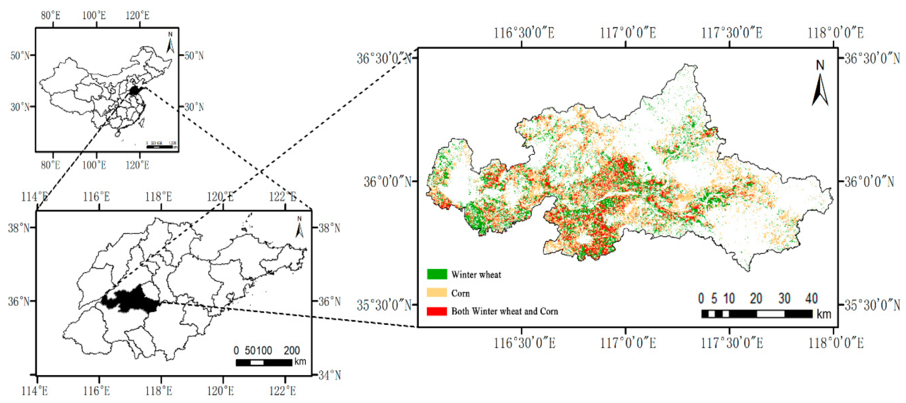
Figure 1. Geographical location and crop distribution for Tai’an City, Shandong Province, China.
Remotesensing 12 00821 g001
Figure 2. An example of an image–label pair used for testing the proposed method: (a) image block, (b) manually-labeled image corresponding to (a), (c) image block, and (d) manually-labeled image corresponding to (c).
Remotesensing 12 00821 g002
Figure 3. Flowchart of the proposed approach. CL: Confidence level.
Remotesensing 12 00821 g003
Figure 4. Structure of the improved RefineNet model used in this study. CB: Convolution Block; FF: Fuse Function; UL: Upsampling Layer.
Remotesensing 12 00821 g004
Figure 5. An example of a histogram.
Remotesensing 12 00821 g005
Figure 6. A description of the modeling progress for a partly connected conditional random field.
Remotesensing 12 00821 g006
Figure 7. Comparison of the segmentation results for 10 randomly selected image blocks: (a) original images, (b) manually-labeled images corresponding to (a), (c) SegNet, (d) SegNet-CRF, (e) SegNet-PCCRF, (f) RefineNet, (g) RefineNet-CRF, and (h) RefineNet-PCCRF. CRF: Conditional random field, PCCRF: Partly connected conditional random field.
Remotesensing 12 00821 g007
Figure 8. Confusion matrices of different models using the GaoFen-2 (GF-2) image datasets: (a) SegNet, (b) SegNet-CRF, (c) SegNet-PCCRF, (d) RefineNet, (e) RefineNet-CRF, and (f) RefineNet-PCCRF.
Remotesensing 12 00821 g008aRemotesensing 12 00821 g008bRemotesensing 12 00821 g008c
Figure 9. Confusion matrices of the different models using the GF-2 image datasets: (a) SegNet, (b) SegNet-CRF, (c) SegNet-PCCRF, (d) RefineNet, (e) RefineNet-CRF, and (f) RefineNet-PCCRF.
Remotesensing 12 00821 g009
Figure 10. The relationship between the average segmentation accuracy and Cgate.
Remotesensing 12 00821 g010
Figure 11. Relationship between average consumed time and Cgate.
Remotesensing 12 00821 g011
Table 1. Model configurations used for the comparative experiments.
NumberNameDescription
1SegNetExtraction using only SegNet
2SegNet-CRFClassic CRF post-processing of SegNet results
3SegNet-PCCRFPCCRF post-processing of SegNet results
4RefineNetExtraction using only RefineNet
5RefineNet-CRFClassic CRF post-processing of RefineNet results
6RefineNet-PCCRFPCCRF post-processing of RefineNet results (method proposed here)
Table 2. The hyper-parameter setup.
Hyper-ParameterValue
Mini-batch size32
Learning rate0.00001
Momentum0.9
Epochs30,000
Table 3. Comparison of the six results.
IndexSegNetSegNet-CRFSegNet-PCCRFRefineNetRefineNet-CRFRefineNet-PCCRF
Accuracy79.01%81.31%83.86%86.79%94.01%94.51%
Precision76.50%78.94%80.68%85.45%91.71%92.39%
Recall73.61%76.24%80.40%79.54%89.16%90.98%
F1-score75.03%77.57%80.54%82.39%90.42%91.68%
Table 4. Statistical comparison of model performance.
IndexSegNetSegNet-CRFSegNet-PCCRFRefineNetRefineNet-CRFRefineNet-PCCRF
Time (ms)301383315293403313