Article

Object-Based Classification Approaches for Multitemporal Identification and Monitoring of Pastures in Agroforestry Regions using Multispectral Unmanned Aerial Vehicle Products

1
MARETEC—Marine, Environment and Technology Centre, Instituto Superior Técnico, LARSyS, Universidade de Lisboa, 1049-001 Lisboa, Portugal
2
Terraprima—Serviços Ambientais, Sociedade Unipessoal, Lda, 2135-199 Samora Correia, Portugal
*
Author to whom correspondence should be addressed.
Remote Sens. 2020, 12(5), 814; https://doi.org/10.3390/rs12050814
Submission received: 2 January 2020 / Revised: 28 February 2020 / Accepted: 29 February 2020 / Published: 3 March 2020
(This article belongs to the Section Remote Sensing in Agriculture and Vegetation)

Abstract

:
Sown Biodiverse Pastures (SBP) are the basis of a high-yield grazing system tailored for Mediterranean ecosystems and widely implemented in Southern Portugal. The application of precision farming methods in SBP requires cost-effective monitoring using remote sensing (RS). The main hurdle for the remote monitoring of SBP is the fact that the bulk of the pastures are installed in open Montado agroforestry systems. Sparsely distributed trees cast shadows that hinder the identification of the underlaying pasture using Unmanned Aerial Vehicles (UAV) imagery. Image acquisition in the Spring is made difficult by the presence of flowers that mislead the classification algorithms. Here, we tested multiple procedures for the geographical, object-based image classification (GEOBIA) of SBP, aiming to reduce the effects of tree shadows and flowers in open Montado systems. We used remotely sensed data acquired between November 2017 and May 2018 in three Portuguese farms. We used three machine learning supervised classification algorithms: Random Forests (RF), Support Vector Machine (SVM) and Artificial Neural Networks (ANN). We classified SBP based on: (1) a single-period image for the maximum Normalized Difference Vegetation Index (NDVI) epoch in each of the three farms, and (2) multi-temporal image stacking. RF, SVM and ANN were trained using some visible (red, green and blue bands) and near-infrared (NIR) reflectance bands, plus NDVI and a Digital Surface Model (DSM). We obtained high overall accuracy and kappa index (higher than 79% and 0.60, respectively). The RF algorithm had the highest overall accuracy (more than 92%) for all farms. Multitemporal image classification increased the accuracy of the algorithms. as it helped to correctly identify as SBP the areas covered by tree shadows and flower patches, which would be misclassified using single image classification. This study thus established the first workflow for SBP monitoring based on remotely sensed data, suggesting an operational approach for SBP identification. The workflow can be applied to other types of pastures in agroforestry regions to reduce the effects of shadows and flowering in classification problems.

Graphical Abstract

1. Introduction

Interest in the data-intensive monitoring of croplands and forests has been spiking recently due to the availability of free Remote Sensing (RS) data from various satellite missions, such as Landsat, Sentinel and others, and the development of Unmanned Aerial Vehicles (UAV) technologies for data acquisition [1,2,3,4,5,6,7,8,9]. Satellite imagery (SI) decreases the cost of repeated data acquisition of the Earth’s surface, promoting the construction of time series based on remotely acquired data. The regular acquisition of information facilitates the development of better algorithms for the identification and monitoring of land cover over time [5,6,10,11]. Close-range photogrammetric surveys using sensors installed in UAV platforms have additional benefits in comparison with free SI, namely at farm or parcel scales, where the spatial resolution of SI cannot provide satisfactory geospatial detail [3]. UAV photogrammetric surveys are a good method to retrieve very high-resolution imagery at smaller scales, despite the need for accurate planning and costly field campaigns. This is the case, for example, in agroforestry landscapes, where different strata of vegetation coexist [3,8].
UAV and SI are frequently used to extract information about land cover types in agroforestry environments. Those products are used for the identification of pastures or grassland, cork oak woodlands and other agricultural fields. Supervised image classification and mapping is increasingly common for the monitoring of grass and pasture parcels [2,4,11]. The automatic supervised classification workflow used in these applications depends on the sensor, type of images, classes nomenclature, algorithms for classification, pixel-based or object-based classification, training and testing data samples and the evaluation of results [12,13], each of which influences computational performance. More recently, Geographical Object-Based Image Analysis (GEOBIA) classification has been replacing traditional classification methods like the pixel-based approach [2,8,14,15]. GEOBIA performs image segmentation based on grouping pixels with similar characteristics, generating sets of homogenous and contiguous segments or regions [15,16,17]. It is particularly recommended for classifying very high resolution imagery, such as UAV products [16,17,18].
Sown Biodiverse Pastures (SBP) are a Portuguese innovation from the 1960s, installed predominantly in the Alentejo region and in Montado agroforestry landscapes, which are of high biodiversity value [19,20]. These high yield pastures can reduce the environmental impacts of grazing systems, mainly through carbon sequestration [21,22,23]. SBP are a mix of up to 20 species or varieties of annual legumes and grasses. Legumes ensure a natural source of nitrogen for pasture growth, enabling the acceleration of nutrient recycling and the increase of carbon sequestration in soils, which contributes to the reduction of carbon emissions compared to production systems based on naturalized grasslands [19,20]. These effects are, however, dependent on the correct management of SBP and their location. The development of techniques and methods for intensively monitoring SBP parcels is becoming increasingly important for the optimization of management practices. Close-range UAV imagery is a promising technique to contribute towards the goal of developing better methods for the monitoring of SBP [4].
At the moment, the algorithms available in literature are incapable of assisting in the remote monitoring of SBP. As many SBP are installed in low-density agroforestry areas or other areas with significant distances between trees [19,20], the tree strata hinder any automatic signal acquisition from the pasture strata. The signature of spectrometric data from SBP is also highly variable in time. SBP have steep seasonal variations throughout their growth cycle, due to weather conditions, agricultural practices and management of the animal production system [19,20]. This temporal variation of the reflectance measured by the sensors can be a limitation for one-period analyses, but also provides an opportunity for improved image classification algorithms [24,25]. Many studies use the temporal patterns of vegetation change for agricultural and forestry applications to construct RS time series-based algorithms for imagery classification, using different band combinations with synthetic bands representing spectral vegetation indices, and integrating different sensors [12,14,24,25,26,27,28,29]. The use of RS time series generates large amounts of data that require computationally efficient classification algorithms [26]. Machine Learning (ML) algorithms are particularly useful for this purpose. In the case of optical satellite imagery, the data available for time series classification depends on the revisiting time of the plots surveyed, and can be affected by cloud coverage and shadows, missing data and satellite/sensor problems [5,26]. UAV imagery is less affected by those problems, but presents additional challenges such as the need to cope with the shadows of objects [2]. Many authors have studied this problem, mainly in open agroforestry farms due to tree shadows [2,30,31], but those methods also have problems of their own. The most common strategies for reducing the effects of tree shadows are the acquisition of UAV imagery at the maximum sun elevation angle, the acquisition of more sources of data or the application of additional radiometric corrections [2,30,31]. To monitor relatively large areas, using maximum sun elevation angles does not work because missions tend to be long enough for the sun to change relative position. Additional data sources may also be unavailable, and the use of further corrections can impose a significant delay on the postprocessing of data.
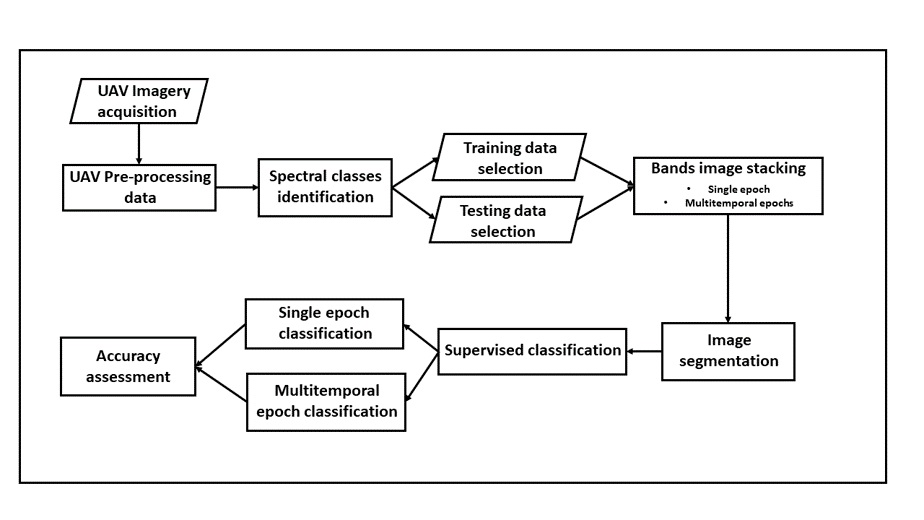
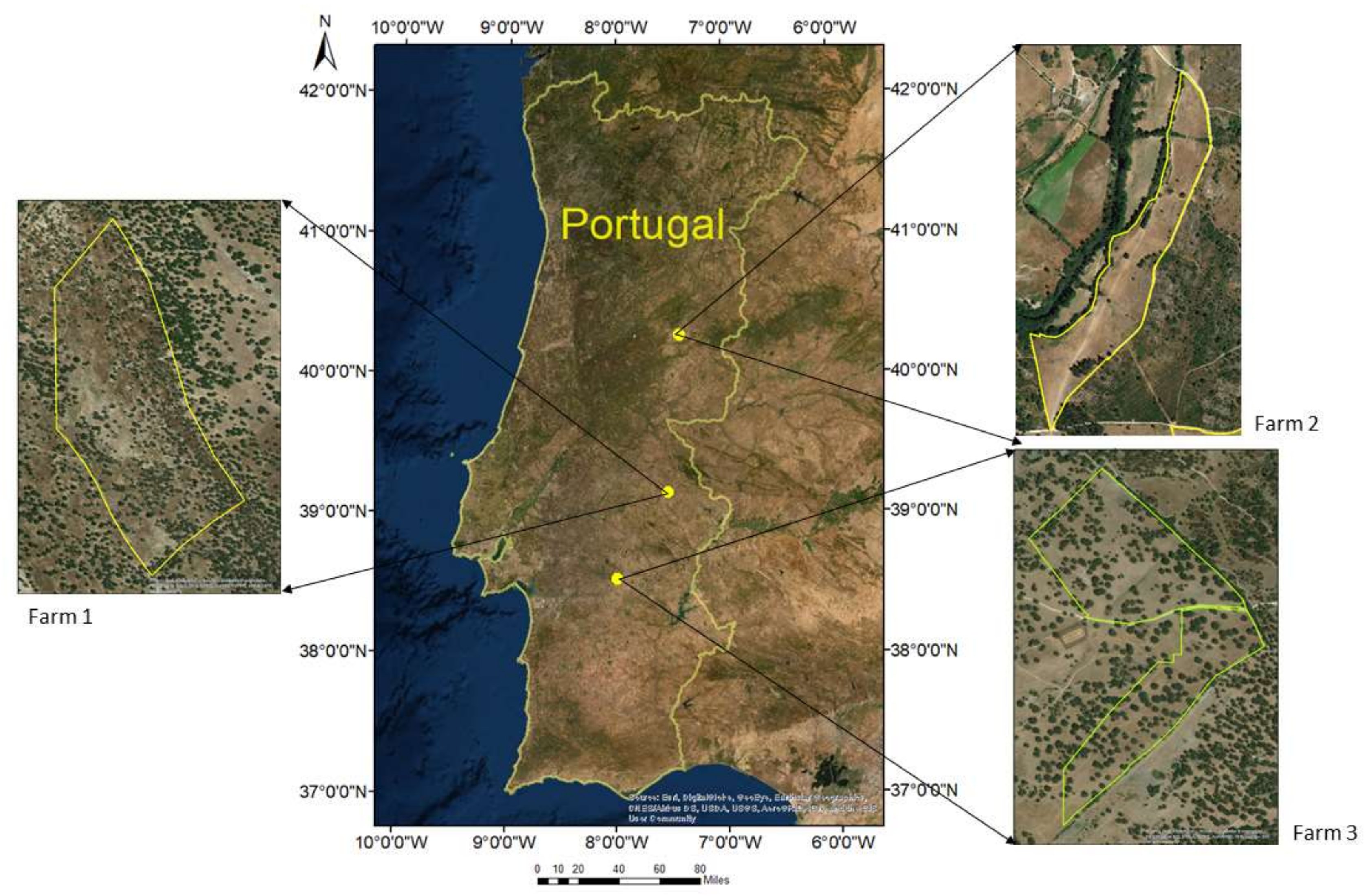
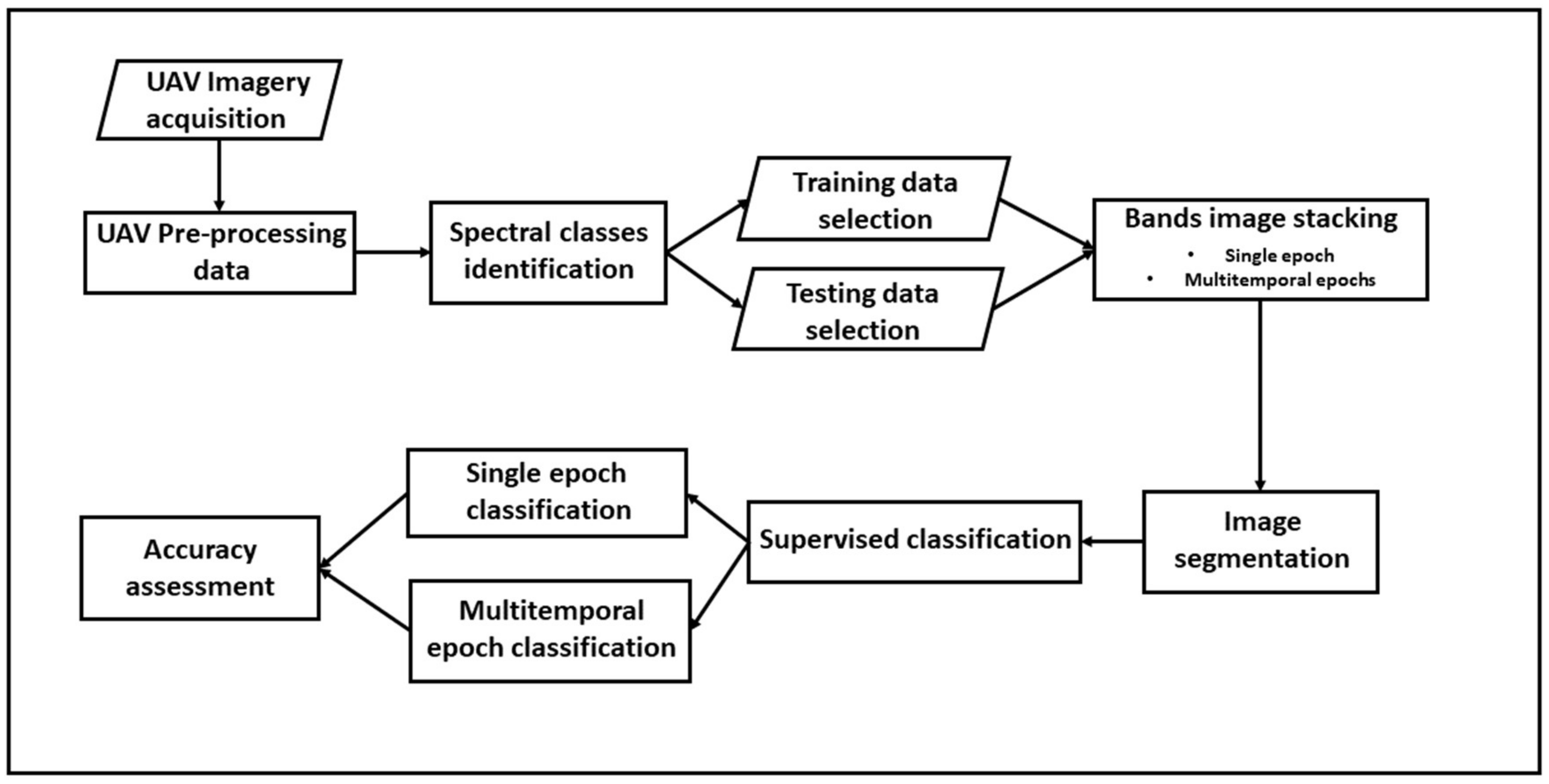
Here, we tested multiple algorithms for the identification and extraction of SBP areas in agroforestry landscapes using GEOBIA classification and UAV surveys conducted in three farms in Portugal. Three ML supervised classification algorithms implemented in the open-source software Orfeo Toolbox (OTB), developed by Centre National d’ Etudes Spatiales [32], were evaluated, namely Random Forest (RF), Support Vector Machine (SVM) and Artificial Neural Networks (ANN). We used two main approaches for the classification of SBP areas: (1) a baseline approach consisting of single period or single image classification, using the period of maximum NDVI; and (2) multi-temporal image stacking, generating a time series considering the temporal variation of pastures in different epochs. This second approach is hypothesized to reduce the misclassification due to shadows and flowers, avoiding the acquisition of additional sources of data or additional radiometric corrections. We obtained one classification map for each procedure and carried out an accuracy assessment of each.
This study was the first application of GEOBIA classification using ML algorithms included in open-source OTB software for SBP classification, in order to implement an operational workflow for SBP and pastures in general remote monitoring in Montado areas. Moreover, we proposed a new multitemporal approach to attenuate for the interference of tree shadows and flower patches that is potentially applicable to other pasture systems.

2. Materials and Methods

2.1. Study Areas

Data for this study were collected in three farms in Portugal, located in the municipalities of Monforte (farm1, Figure 1), Covilhã (farm 2) and Évora (farm 3). The SBP parcels surveyed in each farm covered approximately 27 ha, 25 ha and 19 ha, respectively.
All farms are in central and southern Portugal in the hot-summer Mediterranean climate region, according to the Köppen climate classification system [33]. These farms have a Mediterranean climate characterized by warm temperatures and low precipitation during the dry season (April to September) and a wet season between October and March. The monthly average temperature in all farms between 1971 and 2000 ranged between 11 and 17 °C, and the accumulated yearly precipitation was 585–945 mm [34]. Farm 2 (the northernmost farm) had the lowest monthly temperature and highest precipitation, while farm 3 (the southernmost farm) had the highest monthly temperature and lowest precipitation.

2.2. Classification Procedure

In this paper, we implemented the six-step method illustrated in Figure 2. The stages were: (i) acquisition and preprocessing of photogrammetric UAV imagery; (ii) preparation of data for classification; (iii) training and testing data selection; (iv) image segmentation; (v) classification procedures and (vi) accuracy assessment. Each stage is described in the next subsections.

2.2.1. Data Acquisition and Preprocessing

The acquisition of images was performed using an hexacopter, the TPAHX01 UAV, owned and assembled by the company Terraprima – Serviços Ambientais, Sociedade Unipessoal, Lda (https://www.terraprima.pt/). This UAV was coupled with a Red-Green-Blue (RGB) camera, GitUP Git2, and a Near-Infrared (NIR) camera, MAPIR. The technical features of the images are presented in Table 1
For image acquisition, the first phase consisted of the flight planning performed using the Mission Planner 1.3.68 ® software. Then, the flights were carried out in the dates shown in Table 2 for each of the farms identified in Figure 1. The images were registered, together with the respective geospatial position and elevation using the onboard positioning and navigational system. After the flights, we identified Ground Control Points (GCP) on the field through photointerpretation, namely easily identifiable stones and crossroads with known XYZ coordinates. Those points were used for the orthorectification process. For each of the three farms, a total of 17, 30 and 17 points, respectively, were used. We then implemented a photogrammetric procedure to obtain the aligned orthoimages, the digital surface model (DSM) and the digital terrain model (DTM). Using raw data, common features and objects were identified using overlapping images to retrieve common reference points. Then, a mesh of 3D points was generated and used to calculate the DSM and DTM. Subsequently, the DTM was used to orthorectify the images and, in turn, create the orthoimages. The final orthomosaics for each farm were generated based on the orthoimages. All preprocessing was performed using the Agisoft Photoscan® software. To assess the quality of the orthomosaics, a set of immutable objects (represented by polygons) from a reference orthomosaic was created. Each farm had a set of polygons that was systematically used to visually ensure the overlapping of the orthomosaics in different epochs. The errors introduced by this procedure were not assessed separately, but they are reflected in the final accuracy quantified for the overall method.
The multitemporal analysis required a radiometric calibration to create consistent measurements of the Earth´s surface over time [35]. At the beginning and the end of the flights, we photographed a single calibration board with known reflectance values. We then correlated the known and the mean photographed reflectance values to obtain a linear calibration equation that was applied to the final orthomosaics. The final step needed for processing UAV imagery was the production of an orthomosaic with 0.02 cm of Ground Sample Distance. A total of nine images were used for this study (three images for each study area, see Table 2.

2.2.2. Preparation of UAV Imagery for Classification

We calculated a Normalized Difference Vegetation Index (NDVI) band for each image/epoch using the formulation proposed by Rouse et al. [36]. A delimitation mask was applied to the orthomosaics, corresponding to the parcels indicated in Figure 1. To improve the computational performance, a resampling of the spatial/geometric resolution was made. In this case, we obtained a new geometric resolution of 0.10 m for all bands. After these steps, we performed layer stacking by merging the RGB/NIR reflectance bands with the NDVI and DSM bands for each image acquisition date. The final stage of preprocessing was the stacking of all orthomosaics corresponding to the images acquired at different epochs that are needed for multitemporal classification.

2.2.3. Segmentation Process

Image segmentation was the first step to perform the GEOBIA classification. GEOBIA classification consists of a preliminary clustering of pixels of the input image that returns agglomerated pixels (also called segments). The agglomeration/segmentation process is based on image partitioning in homogeneous areas according to the identification of the elements of the image, usually the shape of objects or spectral homogeneity. The segmentation process results in a vectorization of the objects [18]. This is a nonparametric, iterative and hierarchical clustering algorithm that implements a segmented procedure using hierarchical relationships between segments [18,37]. In the present study, the Large-Scale Mean-Shift (LSMS) [18,32] segmentation algorithm developed in OTB was used to segment the multispectral UAV images. This algorithm can be applied to multispectral images. In OTB, the segmentation process was divided in four main steps: (1) MeanShift smoothing, (2) MeanShift segmentation, (3) MeanShift merging, and (4) MeanShift vectorization [18,32]. We performed multiple tests to identify the most representative segments according to the identifiable objects on images. The variables available to parametrize image segmentation in the LSMS algorithm were the spatial radius (radius of the spatial neighborhood for averaging the pixels), range radius (threshold on spectral signature using Euclidean distance), minimum segment size and size of tiles in pixels (i.e., size of tiles along the X- and Y-axis for tile-processing). Based on a visual inspection and analysis of the preliminary segmentation results, different values of these parameters were tested. The quality of results was assessed by visual interpretation of the segments and the original UAV imagery. The segments were characterized using the respective arithmetic mean, minimum, maximum and standard deviation of radiometric data.

2.2.4. Classification Approaches and Procedures

The classification procedure was performed in OTB. We used four land cover classes: (a) “shadow”, (b) “trees and shrubs”, (c) “bare soil” and (d) “SBP”. Based on the segmentation results, we tested three nonparametric supervised ML algorithms to classify each segment according to the four land cover spectral classes: Random Forest (RF), Support Vector Machine (SVM) and Artificial Neural Networks (ANN). The procedure to select the training data is described in Section 2.2.5. The algorithms were trained using the mean value of radiometric data of segments. These procedures are described in Section 2.2.4.2. After the classification process, the resulting SBP land cover maps were evaluated through an accuracy assessment presented in Section 2.2.6.

2.2.4.1. SBP Classification using RF, SVM and ANN Algorithms

This work used three of the most successful ML algorithms: SVM, RF and ANN. SVM is a nonparametric supervised learning approach. It considers one hyperplane, i.e., the ‘optimal hyperplane’, that divides the data into a predefined number of classes, maximizing the margins between the classes, and minimizing the classification errors [38,39]. SVM incorporates a kernel function to distinguish between classes. Here, in the application of SVM and regarding the kernel type, we tested the linear, sigmoid and gaussian radial basis functions. We also tested the C and Nu support vector classification and distribution estimation (One Class SVM) model-types.
The RF algorithm is based on an ensemble learning for classification and regression. During the training process, RF minimizes the overfitting to produce more accurate classifications [40,41]. RF uses bootstrap aggregation to combine different subsets of decision trees to classify the data. The predicted class, i.e., the classification label of the input vector, is calculated using majority vote. Based on the original data set, this algorithm generates a set of observations called Out-Of-Bag (OOB). OOB data is omitted from the bootstrap training sample and is then used to calculate the accuracies and error rates of predictions [40,41]. For the RF classifier, we varied the maximum depth of the tree, the number of clusters to find a suboptimal split, the maximum number of trees in the forest and the sufficient accuracy (OOB error).
The ANN algorithm comprises a set of interconnected layers of information, where each connection has an associated weight [13]. The networks include one input layer, one output layer and intermediate layers, also known as hidden layers. The number of intermediate layers is variable, as is their size (i.e., the number of ‘neurons’ in each intermediate layer). ANN learn by adjusting the weights of the connections between layers and, consequently, improving the performance of the network. The learning process requires an activation function. The activation function can have multiple functional forms. Throughout the network, the error is back-propagated recursively [42]. We tested resilient backpropagation and simple back-propagation ANN algorithms. We changed the number of neurons in each intermediate layer and tested two different neuron activation functions, namely the Symmetrical Sigmoid function and the Identify function. In OTB version-6.6.1, the Gaussian activation function is not completely implemented. For this reason, this function was not considered.

2.2.4.2. Single Epoch Versus Multitemporal Classification

The classification workflow was implemented using a single epoch classification and a multitemporal classification. For single epoch classification, we considered three collection dates for each farm independently: 7th November, 2017, 17th April, 2018 and 10th November, 2017 (see Table 2 ), for farms 1, 2 and 3, respectively. Those epochs have the maximum NDVI in the sample for each respective farm. For multitemporal classification, an image stacking process was carried out for each farm in order to produce one composite file including all RGB, NIR spectral bands and NDVI and DSM bands for all images available in each farm.
Single epoch classifications needed to include a “shadow” class. The problem with this class is that it changes position between epochs depending on the sun´s different elevation angles at each date of acquisition, exposing different regions of the pasture understory in the vicinity of the tree. Shadow areas are, therefore, mostly pasture areas. The goal of multitemporal classification was to remove the tree shadow class through the use of data from multiple dates. As we used three epochs, the probability that shadows always covered the same pixels in all three was low, which makes the correct identification of the area possible. The “shadow” class was therefore removed from multitemporal classification.
The temporal variability of spectral data has a distinct fingerprint for each land class. Pasture yields vary due to seasonal variations during their growth cycle, agricultural practices, herding, management of animal production system, seasonal flowering among others (Figure 3). These characteristics are difficult to perceive in single epoch classification. Spring flowering, for example, can confuse single epoch algorithms for SBP identification (Figure 3c) because the reflectance of flower patches is significantly different from the reflectance of green biomass. Additionally, those observable patterns are absent from the data for the other land classes. We therefore expected that multitemporal classification would increase the accuracy of SBP classification due to its use of the information provided by the intra-annual variability of pasture vegetation.

2.2.5. Selection of Training Data

We used a stratified sample of training data to perform single epoch and multitemporal classifications. First we defined the minimum number of sets required for training. As a rule of thumb, we assumed that to obtain classification maps with less than 12 classes, as in the case of this study, each training class should comprise a minimum of 50 samples, as recommended in the literature [12] to obtain a statistically significant representation of the classes in the image.
The basis for the choice of training data was the visual interpretation of images and field-knowledge about the farms. Depending on the class, we selected between 51 and 420 training polygons for each land cover class. Two main criteria were used for determining the number of polygons. First, the number of polygons chosen was directly proportional to the estimated frequency of each class in the images. Second, it was set to ensure minimum statistical representativity during training (for the less represented classes, in this case, “bare soil”) and prevent the training polygons to take more than 2% of all segments [12]. The bare soil class therefore had the lowest number of training areas, with 51 polygons. The highest number of polygons, 420, was used for the most frequent class, i.e., “SBP”. The “shadow” class is absent from the multitemporal classification, and therefore, training polygons belonging to the “shadow” class in individual images were classified as “SBP”. Consequently, we expected the area classified as SBP in the multitemporal approach to increase. In Appendix A (see Table A1) we show the number of training polygons used to train the classification models using the SVM, RF and ANN algorithms.

2.2.6. Accuracy Assessment

The accuracy assessment of classification results was performed by using samples points for each land cover class. Randomly selected sample points were compared with predictions of class membership returned by each algorithm described in Section 2.2.4.2 (see Table A8). For each classification map, we calculated the confusion matrix, the overall precision [12], user’s and producer´s accuracy [12] and the kappa index [12].

3. Results

3.1. Preliminary Results of RF, SVM and ANN Classifications

We started by testing the methodological choices indicated in Section 2.2.4.1. Tests performed with SVM showed that the default values of OTB presented the best results. By changing the cost parameters (C and Nu), the preliminary results were similar to the results obtained with their default values (1 and 0.5, respectively). The Linear kernel showed the best performance in comparison with the remaining kernel functions (Gaussian radial basis, polynomial and sigmoid). Thus, the default SVM parameters were used to perform the classification procedures. After several tests to study the RF parameters, we considered a maximum depth of the tree of 5. The minimum number of samples in each node was 10, the number of clusters was set 10 and the OOB error was set at 0.01. For ANN parametrization, the resilient back-propagation training method showed better performance than the back-propagation algorithm. Increasing the number of intermediate layers and changing their respective sizes did not improve the results. Regarding the neuron activation function, the symmetrical sigmoid function returned the best performance in comparison with the identify function. Due to these results, we selected the resilient back-propagation algorithm for training the ANN with one intermediate layer with 100 neurons activated according to a symmetrical sigmoid function.

3.2. Single Epoch Classification

Table 3 shows the overall accuracy and kapa index for all single epoch classifications. The overall accuracy for all classified maps was higher than 79% for all farms and for all algorithms tested. The RF algorithm, in all farms, had the highest overall accuracy and kappa index, i.e., above 92% and 0.88, respectively. ANN had the lowest accuracy for all three farms. Comparing the three farms, the application of the classification algorithms in farm 3 had higher accuracy and kappa index. The bare soil class had the smallest classified area (less than 8% of each farm). In farms 2 and 3, ANN classified a higher percentage of the area as trees and shrubs than the RF and SVM algorithms (see Appendix B). This happened because land classified by the ANN algorithm as “trees and shrubs” was classified by SVM and RF algorithms as “SBP” (see Appendix BFigure A1, Figure A2, Figure A3 and Figure A4). Figure 4a,b visually depict the accuracy level of the identification of shrubs by RF classification in farm 2. In farms 2 and 3, the fraction of the area classified as SBP by RF and SVM was similar. All algorithms identify an area of more than 50% of all farms as SBP (Figure 5). The SVM algorithm classifies a higher percentage of the area as SBP than the ANN and RF classifiers (bar charts in Figure 5). Table A2, Table A3 and Table A4 are the confusion matrices (Appendix A) of single epoch classification. The SVM and ANN algorithms display more confusion between SBP and bare soil classes than the RF algorithm (cf. also Figure 5d). The area of SBP may, therefore, be underestimated, as SBP areas may have been classified as bare soil.

3.3. Multitemporal Classification

Table 4 shows results for overall accuracy and Kappa indices for the multitemporal classification performed with SVM, RF and ANN algorithms. Multitemporal classification using the RF algorithm yields the highest overall accuracy in all farms and approaches (cf. Table 3 and Table 4). Compared with the single epoch classification, the multitemporal approach increased the respective accuracy by 3.9 percentage points for farm 1, 0.3 for farm 2 and 0.9 for farm 3. The ANN algorithm had already performed the worst in the single epoch approach and in terms of overall accuracy for multitemporal classification. Furthermore, the ANN multitemporal algorithm showed lower overall accuracy compared to single epoch classification for farms 2 and 3. Figure 6 presents the classification maps and bar charts for multitemporal approach in all farms using the RF classifier.
Analyzing Figure 5 and Figure 6, the area classified as SBP increased as a percentage of the total in comparison with single epoch classification. This result was expected because in multitemporal classification, we considered tree shadows as SBP areas. In general, the percentage of area classified as trees and shrubs was similar for both classification approaches in farm 3. In farm 1, the area of trees and shrubs was approximately 10% higher using RF multitemporal classification than the single epoch approach. In farm 2, multitemporal classification resulted in lower three coverage than single epoch classification, particularly with the ANN algorithm (31% compared to 10%) and SVM (11% and 6%).
The multitemporal classification of SBP was more consistent across algorithms than single epoch classification had previously been. Comparing bar charts in Figure 5 and Figure 6, the multitemporal approach with RF and ANN identified approximately the same area of SBP, particularly in farms 1 and 2. Additionally, multitemporal classification solved issues with the misidentification of objects in single epoch classification, particularly in farms 1 and 3. In farm 1, using single epoch classification, some areas were correctly classified as shadow using ANN and RF but misclassified as bare soil using SVM (Appendix A, Figure 1 and Figure A2). Multitemporal SVM classification identified those areas as SBP, which is the most likely class for those objects. Table A5, Table A6 and Table A7 present the confusion matrices of SVM, RF and ANN of multitemporal classification, showing the reduction of underestimation of SBP areas in relation to the bare soil class.
Figure 7 presents a small region in farm 3 (Figure 7a,b) and the respective results of multitemporal classification using ANN (Figure 7c), SVM (Figure 7d) and RF (Figure 7e). All algorithms were able to distinguish between SBP, including flower patches, and bare soil. In this case, RF reduces the misclassification of flower patches in comparison with the remaining algorithms, while SVM is more accurate for the reduction of misclassification due to shadows. SVM is particularly powerful for accurately tracing the boundary between the shadows and trees (see Figure 7a,b,d).

3.4. Producer´s and User´s Accuracy Results

Table 5 shows the producer’s and user´s accuracies using the ANN, RF and SVM classifiers in the three farms and for single epoch and multitemporal classification approaches. For most cases presented in Table 5, the user’s and producer’s accuracy is higher than 70%. The RF and SVM algorithms are more accurate than the ANN algorithm. Multitemporal classification of SBP has higher user´s and producer’s accuracies than the single epoch approach, particularly in farm 1. In farm 3 the bare soil class has the lowest producer´s accuracy for RF and SVM (15% and 14%, respectively), due to the confusion between the bare soil area classified as trees/shrubs in the multitemporal classification.
The user’s accuracy for bare soil was higher for farms 2 and 3 (100%), regardless of the algorithm. The producer’s and user’s accuracies for SBP are close to or higher than 90% in the majority of cases, with the exception of the ANN classifier in farms 1 and 2 (for user’s accuracy). The producer´s accuracy of trees and shrubs in farm 2 is lower in multitemporal classification than single epoch classification, particularly for the ANN algorithm.

4. Discussion

Out of the many methodological options studied in this paper for identifying SBP areas using RS data, the option that stands out is multitemporal classification using RF. The RF classifications were more accurate than the SVM and ANN classifications (see Table 3, Table 4 and Table 5) in both single epoch and multitemporal classifications. However, in general, SBP and other classes were identified with high accuracy (overall accuracy higher than 79%), regardless of the algorithm. A previous study applied RF and SVM to identify grassland, trees and bare soil land classes in non-SBP Montado areas using UAV imagery and OTB [2]. That study also determined that the RF and SVM algorithms had a similar accuracy (~97% and ~95%, respectively), which is similar to the performance we obtained.
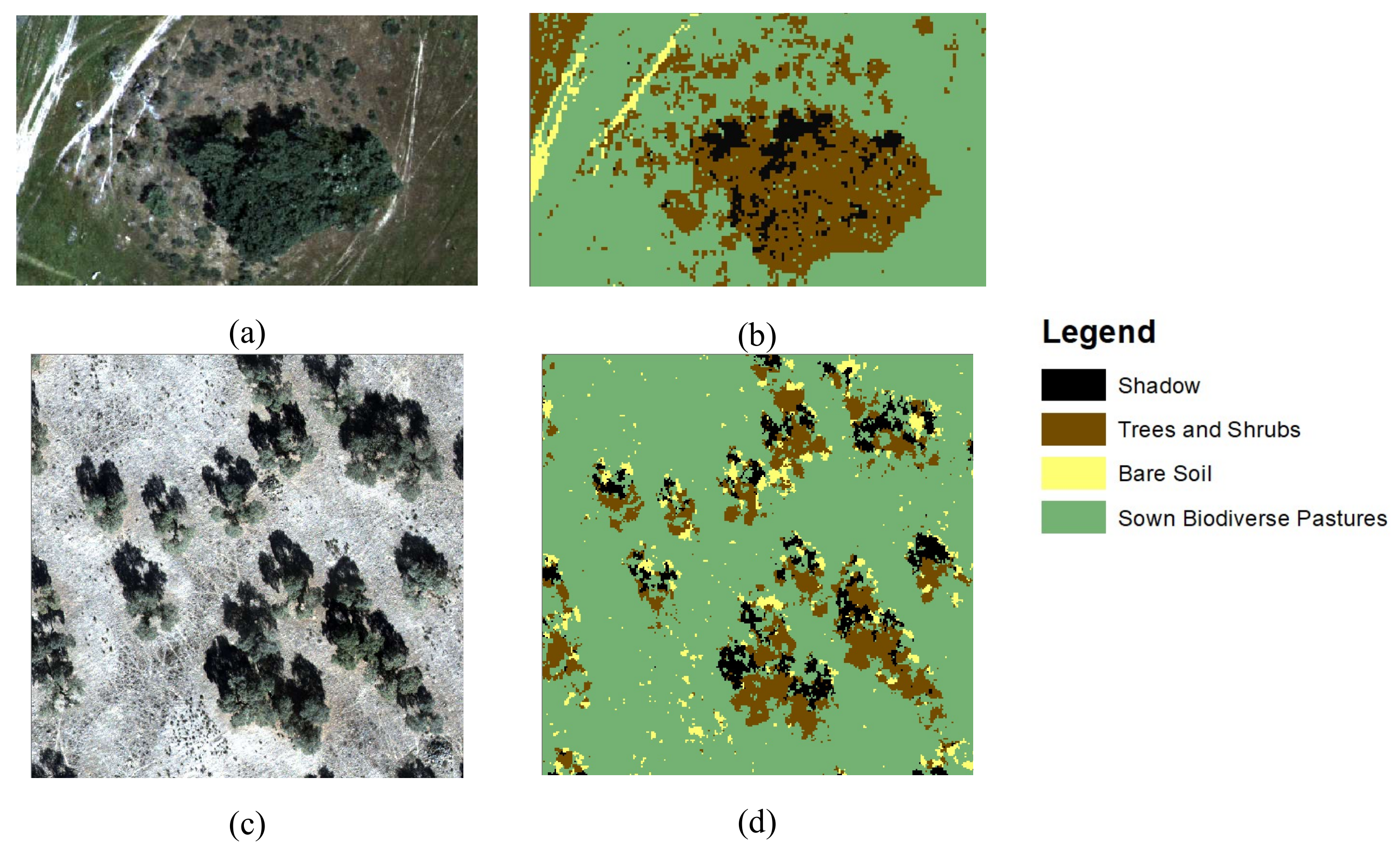
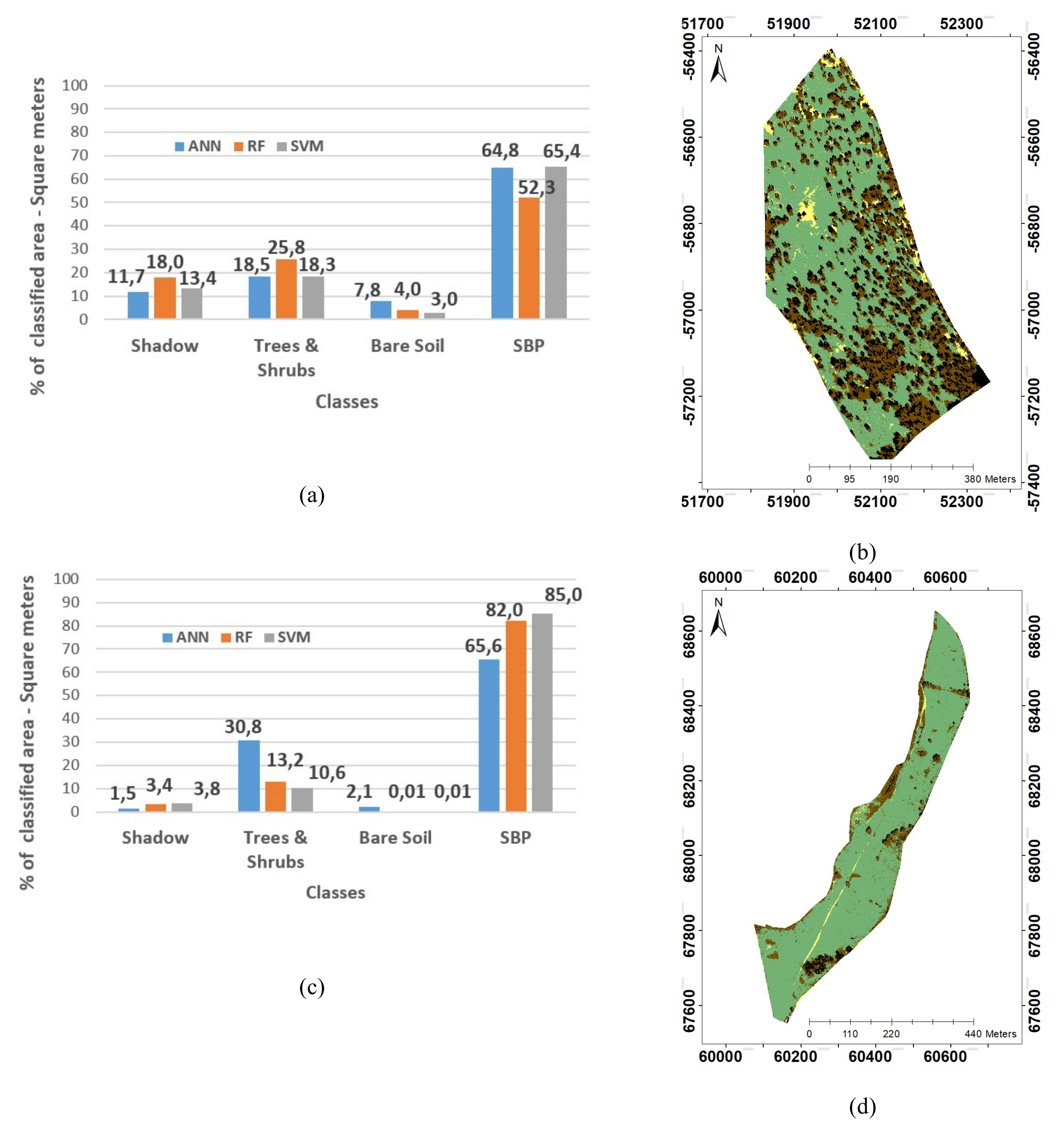
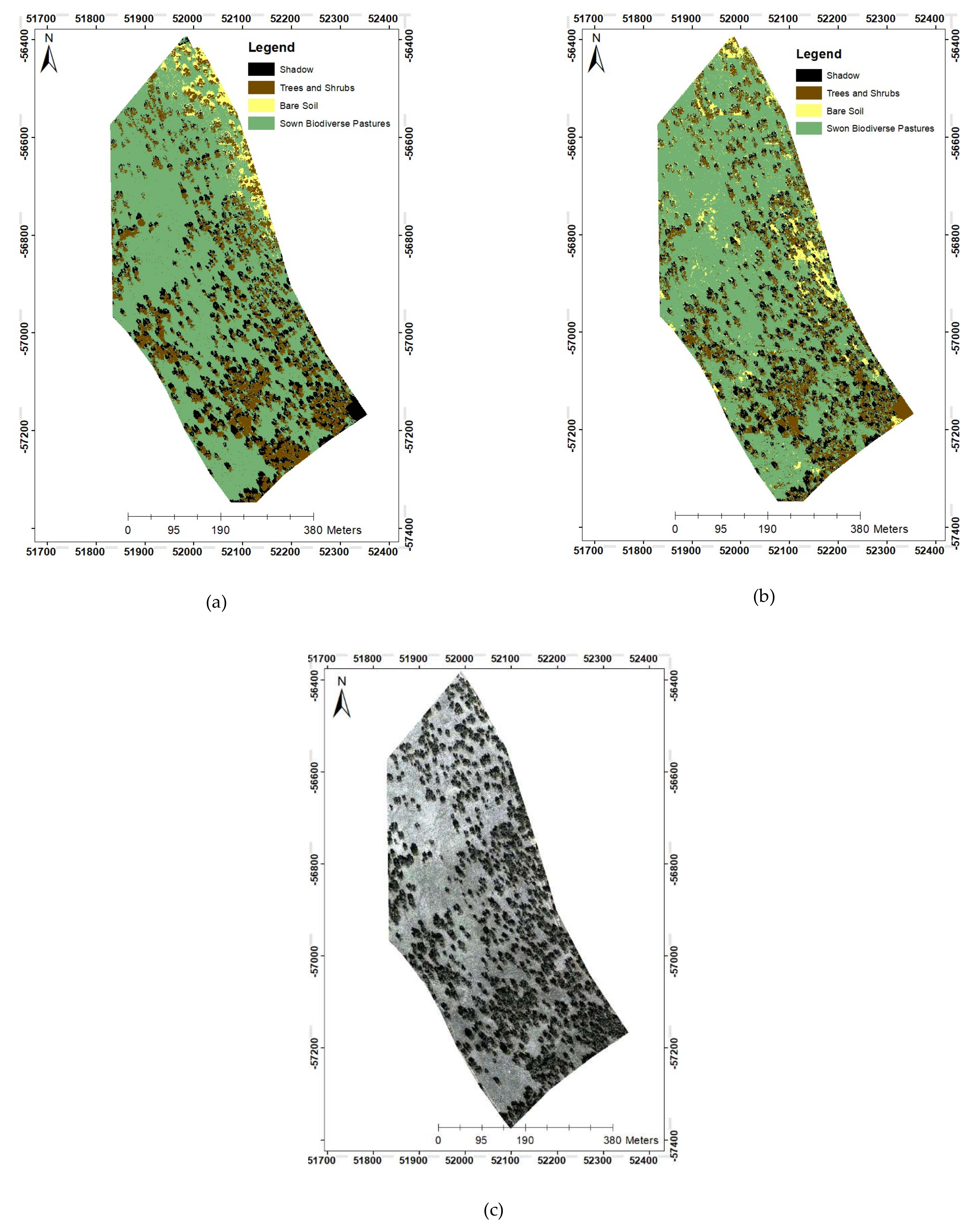
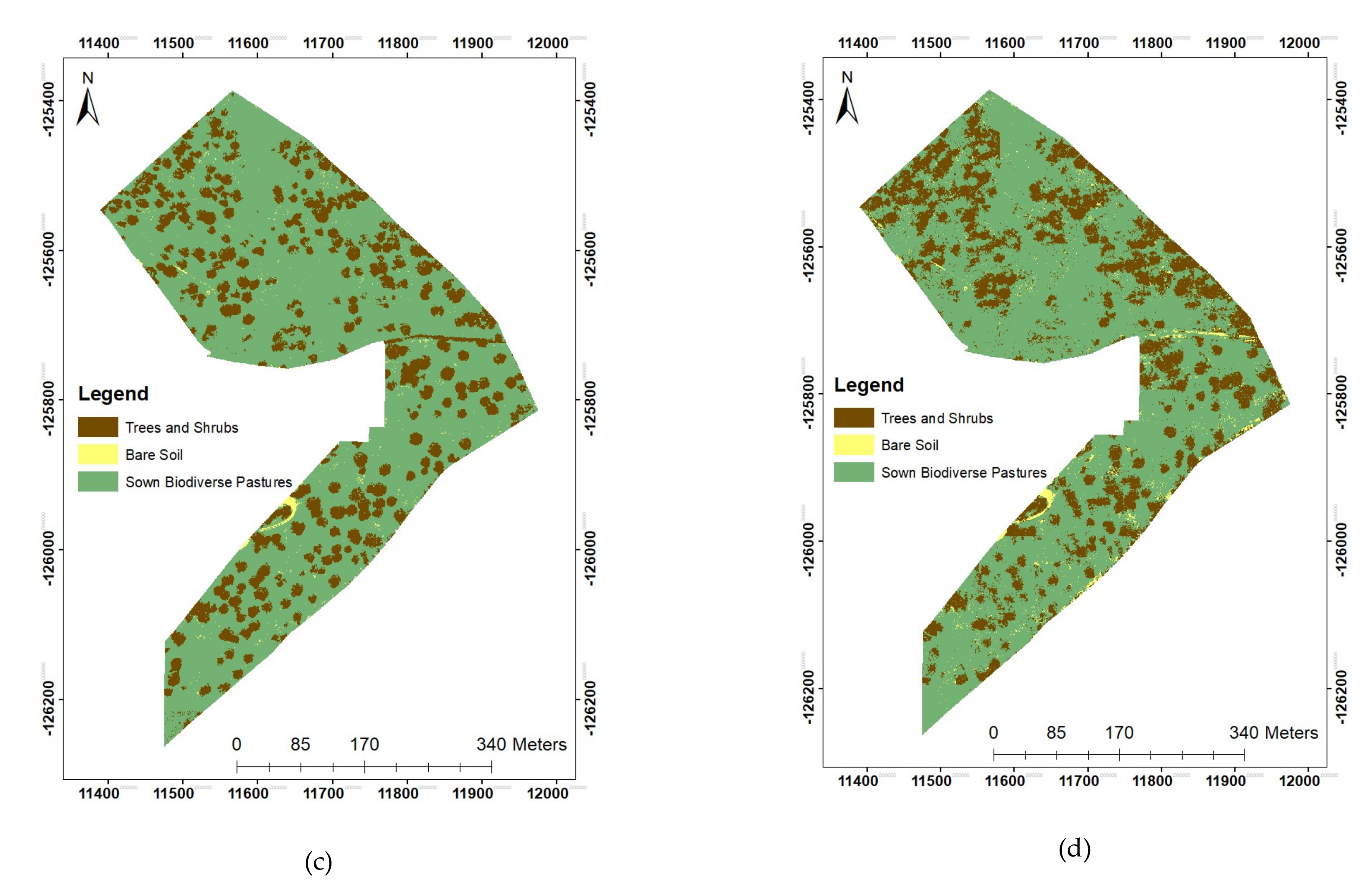
A visual analysis of classification maps shows a common error in classification in all farms, which is mostly prevalent in ANN and RF algorithms; some objects that represent the boundary of the shadows were classified as trees and shrubs (see Figure 5). This confusion is due to the spectral transition from the shadow to the pastures. This caused an increase of 10% in the size of the area classified as containing trees in farm 1 using the multitemporal RF classification. This problem has also been reported elsewhere in the literature for trees and shadow classification in cork oak environments [2], but at the moment, we are unable to explain why some algorithms are more sensitive than other to this issue.
The bare soil class covered less than 8% of the parcels. This class included mostly the small roads that exist in the farms, tracks created by frequent movements of animals and some smaller regions of confusion with flower patches in the spring. Although additional data would be needed to fine-tune the algorithms and more accurately classify those regions of the image, the largest and most clearly visible bare soil patches were correctly identified. The lowest producer´s accuracy for the bare soil class was found in farm 3 for multitemporal RF and SVM classifications. Most bare soil areas in this farm were correctly identified. However, in some of the images, shrubs display an absence of vigorous leaves, and can be easily confused with soils. This confusion could have lowered the producer´s accuracy of this class.
Trees and shrubs have similar spectral behavior and shapes, and for this reason, we merged them into a single class. For this class, the DSM had an important role in distinguishing trees from the remaining classes, namely SBP, due to the high altimetric differences [2,11,43]. However, within this class, segmentation was difficult owing to the small dimensions of the shrub objects. Thus, we chose a lower-scale segmentation in order to detect slight spectral and radiometric differences in shrubs and trees, testing multiple values of range radius to avoid over- and under-segmentation. High range radius (over 10) tended to result in under-segmentation of trees and shrubs, hampering the correct identification of shrubs. Low range radii resulted in over-segmentation, and consequently, poor computational performance. Thus, we adopted a range radius between 6 and 8, which worked better for low scale segmentation, and correctly identified most visible shrubs. This segmentation problem in very high-resolution images has been widely reported in the literature [2,44], with some authors suggesting that a range radius between 6 and 7 can lead to satisfactory results in segmentation using OTB [2]. In some studies [14], multitemporal classification increased the number of segments due to the temporal variability of classes. Our segmentation process led us to the same conclusion, mainly for the SBP class.
Still, RF and SVM were capable of correctly identifying most trees. The main issues were found in multitemporal classification using ANN, which erroneously identified some SBP areas as trees and shrubs in farms 2 and 3, decreasing overall accuracy in comparison with single epoch classification. Raczko and Zagajewski [45] compared RF, SVM and ANN to identify trees in forested areas. They discussed and concluded that the RF and SVM algorithms are easier to parameterize than ANN. This conclusion also agrees with the results presented and discussed here about tree classification. Testing why multitemporal ANN classification displays those issues was beyond the scope of this study, but it should be regarded as a topic of future research.
Multitemporal classifications had higher overall accuracies and kappa indices than single epoch classifications in most cases because it took into account the temporal variability of vegetation and climate [46]. The land cover-specific variability of reflectance of the different strata was particularly important to distinguish between trees/shrubs and pasture. While perennial leaf trees, which are the most frequent in these Montado regions, remain approximately constant in shape and color throughout the year, the characteristics of SBP vary widely. SBP go through a green stage in autumn/early winter, flower and see a boom in productivity in the spring, and completely dry out in the summer. These changes are clearly seen in our UAV data for the study period. Farm 1 is particularly sensitive to the classification approach, as overall accuracy from multitemporal classification was about 4% higher. In our study, we only used three epochs to evaluate the influence of temporal variability. A previous study [46] considered different time steps of UAV imagery classification. They found that the overall accuracy of results increased by 3% with two or more images compared with using a single image. Our results agree with this observation. This could potentially indicate that the results would be unaffected by adding more epochs. However, the improvement in accuracy is unevenly distributed between the classes and particularly affects classes with lower area (such as bare soil, in our case). The addition of further epochs comes at a cost due to the time and resources involved to carry out UAV flights, and therefore, the cost-benefit of adding more epochs should be carefully evaluated in the future. There are additional approaches for multitemporal analyses that can be tested. For example, very high resolution (VHR) satellite data can be used to increase the temporal resolution of UAV images through fusion of data acquired with different spatial and radiometric resolution, such as those based on concept of “super-resolution” [47].
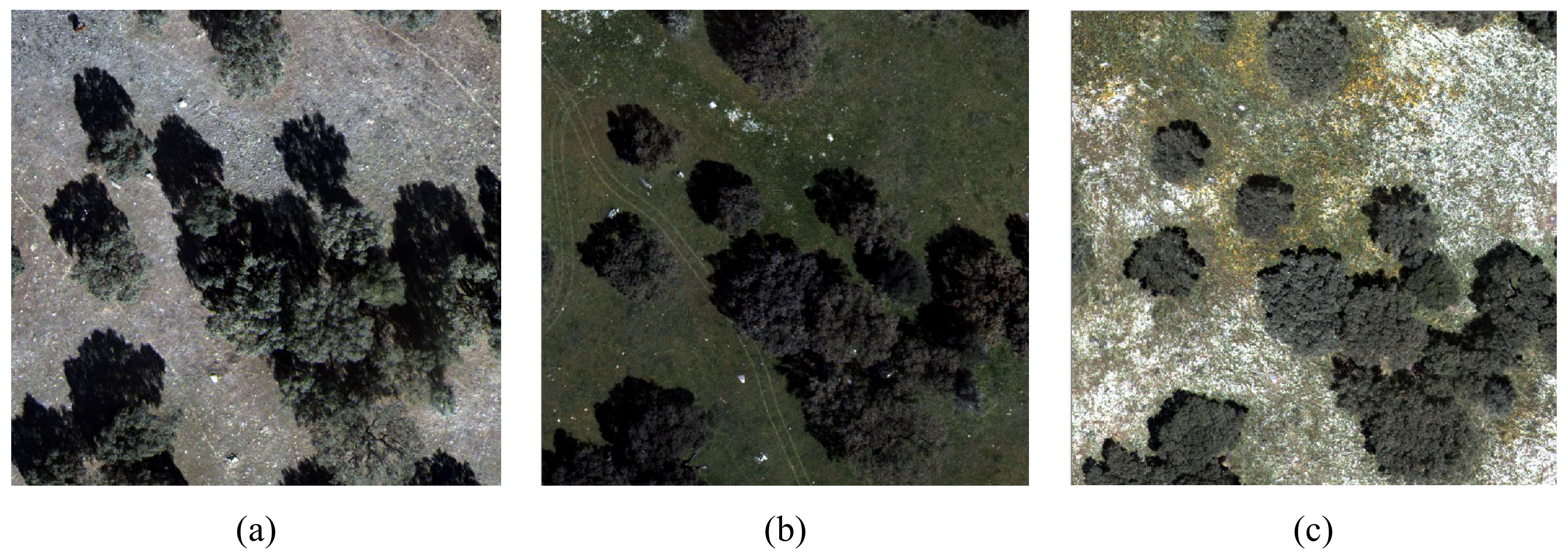
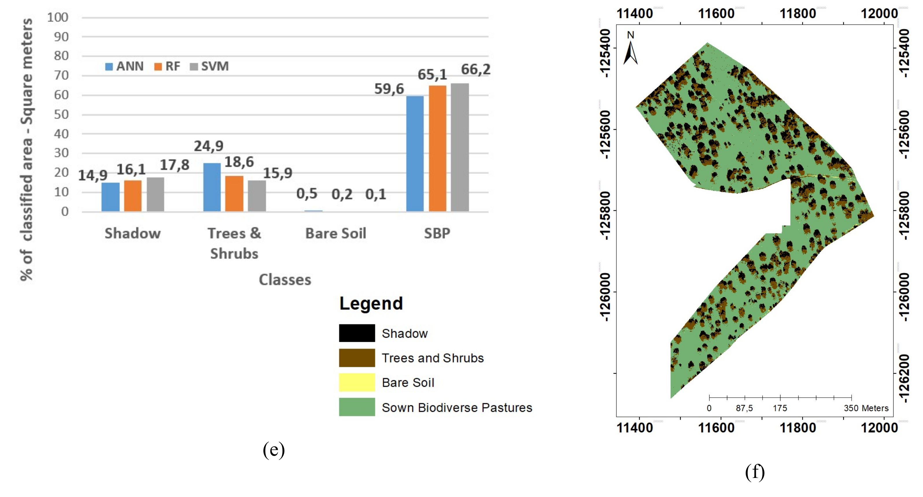
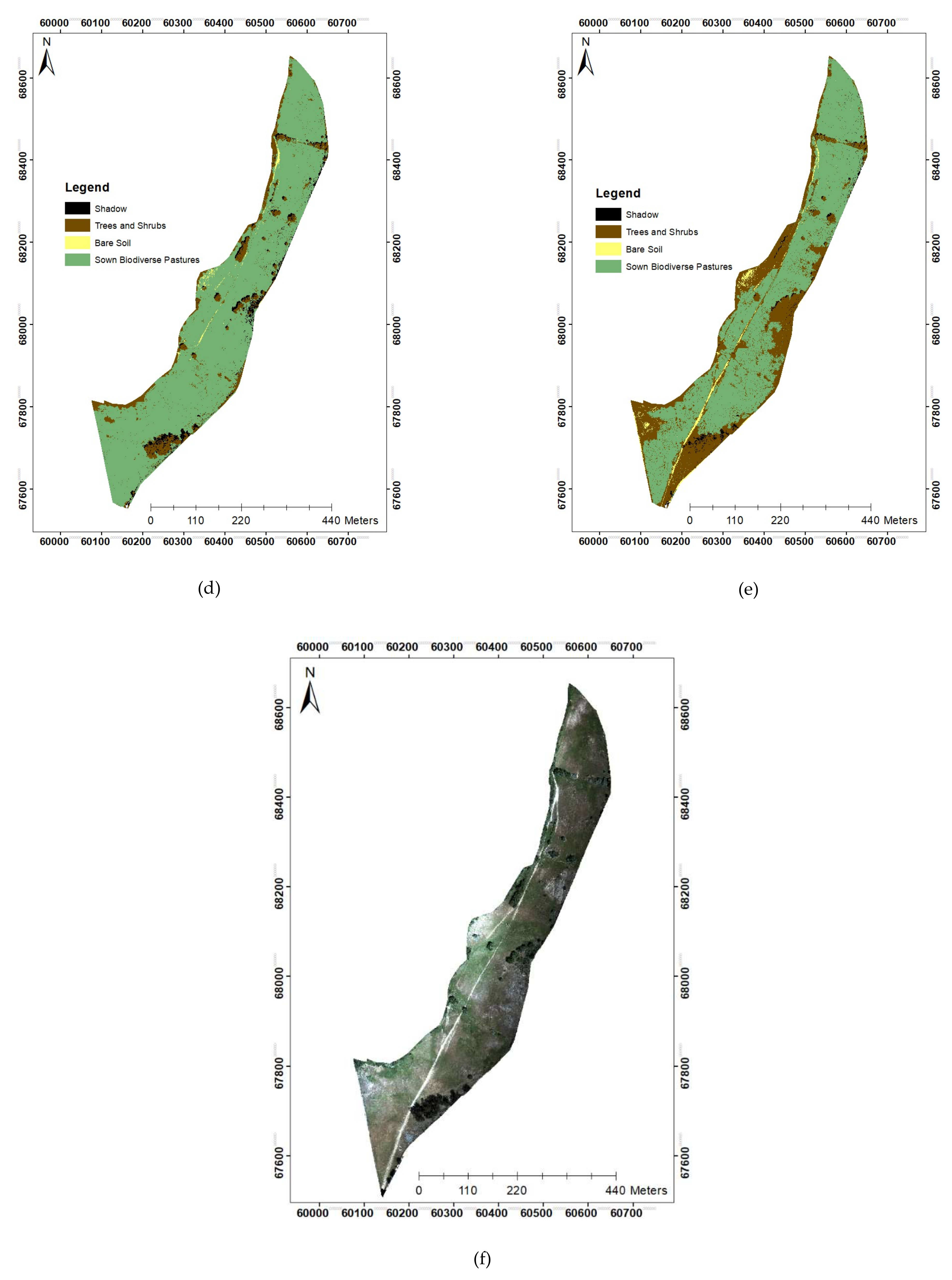
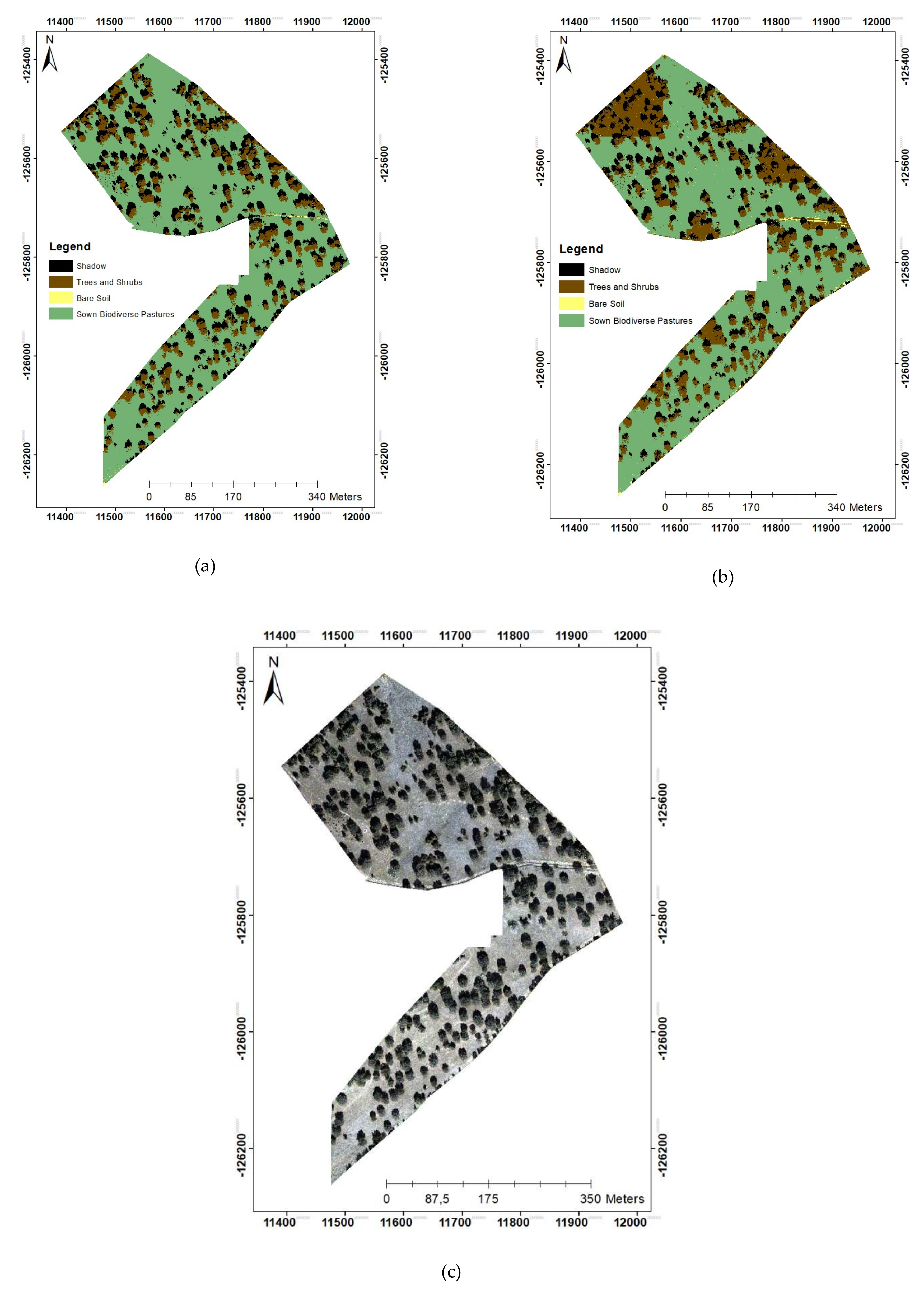
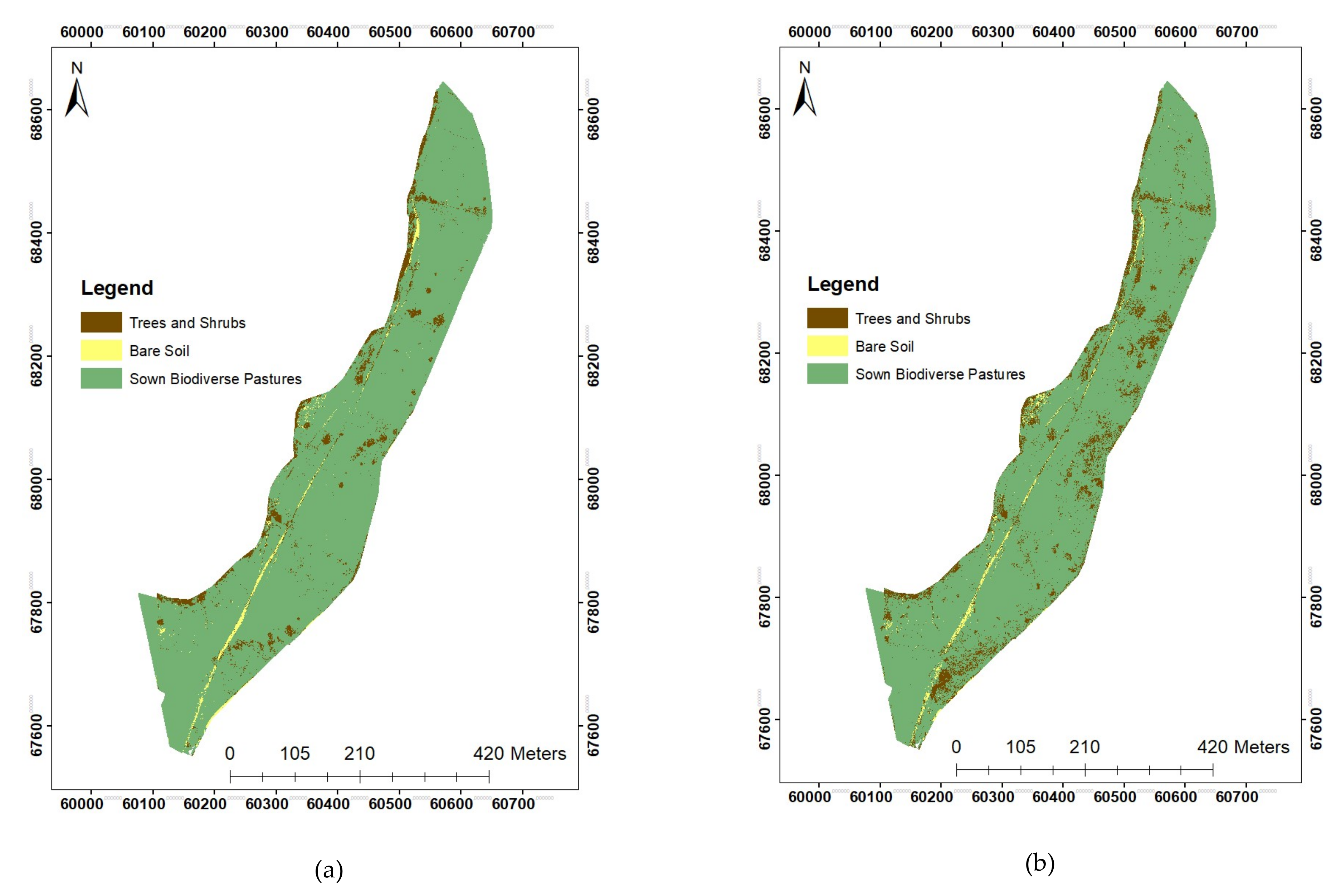
Finally, farm 3 displays very prominent flowering in SBP areas (Figure 3) during Spring, particularly due to Chamaemellium mixtum. The radiometry of those flowers is very similar to bare soil radiometry. Therefore, single epoch classification tends to underestimate SBP area by assigning flower patches to the bare soil class. Multitemporal classification fixed the majority of these issues, as most flower patches were classified as SBP (Figure 5 and Figure 6). Similarly, the effect of tree and shrub shadows was attenuated through multitemporal classification. This problem is widespread in RS-based classifications of land classes in agroforestry systems, and was dealt with here without the need for additional radiometric correction methods [2,31]. Decreasing the effects of shadows and flowers enabled us to identify SBP areas with greater accuracy, as shown by the increased producer and user accuracy of the SBP class. The approach developed here is therefore promising as a general strategy to reduce similar effects in classification problems for other grassland systems in open Montado agroforestry areas. The reduction of the misclassification due to shadows and flowers in multitemporal classification also reduced the differences of estimated total SBP area between the algorithms, which were sharper for single epoch classification. Thus, the multitemporal classification harmonized the performance between different classifiers/algorithms.

5. Conclusions

5.1. Final Considerations

This study was performed to address an increasingly pressing need for RS-based classification of pastures in agroforestry regions, through the development of an accurate workflow capable of correctly identifying pasture areas, even in the presence of trees shadows and flowers. Both effects confuse algorithms and lead to the underestimation of pasture areas using data collected on one singular date. We showed here that a multitemporal approach is crucial in order to deal with the effects of tree shadows and flower patches. This approach works mostly due to the radiometric variability of SBP, compared to the trees and other objects in the ecosystem. To our knowledge, this was the first application of multitemporal classification that successfully decreased misclassifications due to shadows and flowers without requiring additional corrections. Prior approaches resorted to physical- or image-based correction methods to identify shadows or the application of multisource data fusion to fill shadowed areas. This study also applied for the first time GEOBIA classification and ML algorithms to identify SBP in Portugal. Although the type of ML algorithm made some difference, with RF being the most accurate, the most important methodological choice for obtaining accurate results was the use of multitemporal classification. The workflow presented here enables the identification of SBP area with an overall accuracy that is always higher than 79%, regardless of the approach. The results presented here are a first step towards the operationalization of remote data-based SBP monitoring, which will be an essential feature of any future environmental and agronomic monitoring system.

5.2. Future Work

This work introduced multiple aspects for consideration in future research. One aspect that should be explained and overcome is the confusion in the boundary of shadows displayed by ANN and RF classifiers due to the spectral transition from shadow to pasture/tree segments. Also, we intend to improve the tree segmentation and classification procedures. Devising alternative efficient approaches to reducing the effects of shadows in single epoch classifications is also a topic worthy of further exploration in future studies. As it is necessary to simultaneously increase the temporal resolution of the data and reduce the costs and efforts of acquisition of new UAV data, one possible way forward is to use methods that combine UAV data with VHR satellite imagery. The results here were mainly evaluated for SBP. In the future, the workflow can be easily applied to other types of pasture in agroforestry systems.

Author Contributions

Conceptualization of study: R.F.M.T., T.D., T.G.M. and P.V. Data acquisition by photogrammetric UAV surveying and preprocessing of the images: N.R.R., I.G. and M.L.M. Methods, results and discussion analysis: P.V., T.G.M. and R.F.M.T. Most of the writing: P.V. and M.L.M. Revision of document: all of authors. All authors have read and agreed to the published version of the manuscript.

Acknowledgments

This work was supported by Fundação para a Ciência e Tecnologia through projects “Animal Future – Steering Animal Production Systems towards Sustainable Future” (SusAn/0001/2016), “LEAnMeat - Lifecycle-based Environmental Assessment and impact reduction of Meat production with a novel multi-level tool” (PTDC/EAM-AMB/30809/2017), “GrassData - Development of algorithms for identification, monitoring, compliance checks and quantification of carbon sequestration in pastures” (DSAIPA/DS/0074/2019), and by grants SFRH/BD/115407/2016 (T. Morais) and SFRH/BPD/111730/2015 (R. Teixeira). The work was also supported by FCT/MCTES (PIDDAC) through project LARSyS - FCT Pluriannual funding 2020-2023 (UIDB/EEA/50009/2020), by Portugal 2020 through project “ModelMeat - Modelo de Optimização de Ambiente e Qualidade do Produto para Serviços de Apoio à Competitividade dos Agentes da Fileira da Produção Animal Extensiva” (nr. 017630), and by Programa de Desenvolvimento Rural (PDR2020) through “Viabilização de pastagens semeadas biodiversas através da otimização da fertilização fosfatada” (PDR2020-101-030690) and “GO SOLO: Avaliação da dinâmica da matéria orgânica em solos de pastagens semeadas biodiversas através do desenvolvimento de um método de monitorização expedito e a baixo custo” (PDR2020-101-031243).

Conflicts of Interest

The authors declare no conflict of interest.

Appendix A

Table A1. Number of polygons used for training for each class in single epoch and multitemporal classification. SBP – Sown Biodiverse Pasture.
ClassFarmSingle EpochMulti-Temporal
ShadowFarm 1154-
Farm 2232
Farm 3198
Trees /ShrubsFarm 1226226
Farm 2257257
Farm 3207207
Bare SoilFarm 1120176
Farm 25151
Farm 352100
SBPFarm 1212366
Farm 2220452
Farm 3213417
Table A2. Confusion matrix of single epoch classification performed with the Support Vector Machine (SVM) classifier, where F1 - farm 1, F2 - farm 2 and F3 - farm 3.
SVM Single EpochGround Truth
1234Total
F1F2F3F1F2F3F1F2F3F1F2F3
Classified1F1185 34 0 0 219
F2 187 3 0 0 190
M 1835 180 0 92024
2F14 490 0 12 506
F2 10 407 0 6 423
F3 2 8376 10 218409
3F112 6 52 4 74
F2 0 0 122 0 122
F3 0 0 1206 01206
4F146 75 18 1198 1337
F2 4 158 293 1120 1575
F3 111 1130 448 2115322842
Total 247201194860556896867041516641214112621183
Table A3. Confusion matrix of single epoch classification performed with the Random Forest (RF) classifier. F1 - farm 1, F2 - farm 2 and F3 - farm 3.
RF Single EpochGround Truth
1234Total
F1F2F3F1F2F3F1F2F3F1F2F3
Classified1F1234 31 0 0 265
F2 190 6 0 0 196
M 1806 12 0 01818
2F15 530 0 29 564
F2 8 418 0 8 434
F3 31 8503 13 308577
3F10 12 70 7 89
F2 0 0 414 0 414
F3 0 1256 01256
4F18 32 0 1178 1218
F2 3 144 1 1118 1266
F3 111 1171 395 2115322830
Total 247201194860556896867041516641214112621183
Table A4. Confusion matrix of single epoch classification performed with the Artificial Neural Networks (ANN) classifier. F1 - farm 1, F2 - farm 2 and F3 - farm 3.
ANN Single EpochGround Truth
1234Total
F1F2F3F1F2F3F1F2F3F1F2F3
Classified1F1172 8 0 3 183
F2 153 3 0 0 156
F3 1792 55 0 01847
2F118 400 0 25 183
F2 45 455 1 22 523
F3 52 8529 25 7719377
3F11 2 38 34 75
F2 0 0 348 0 348
F3 0 0 1383 01383
4F156 195 32 1152 1435
F2 3 110 66 1104 1283
F3 104 1102 256 2041221874
Total 247201194860556896867041516641214112621183
Table A5. Confusion matrix of multitemporal classification performed with the Support Vector Machine (SVM) classifier. F1 - farm 1, F2 - farm 2 and F3 - farm 3.
SVM Multiple EpochGround Truth
234Total
F1F2F3F1F2F3F1F2F3
Classified2F1526 0 109 635
F2 227 5 25 257
F3 9423 1167 24410834
3F10 39 0 39
F2 0 255 0 255
F3 0 232 103338
4F149 31 1352 1432
F2 295 155 1302 1752
F3 263 265 2278123309
Total 57552296867041516641461132723131
Table A6. Confusion matrix of multitemporal classification performed with the Random Forest (RF) classifier, F1 - farm 1, F2 - farm 2 and F3 - farm 3.
RF Multiple EpochGround Truth
234Total
F1F2F3F1F2F3F1F2F3
Classified2F1571 0 36 607
F2 395 1 29 425
F3 9599 51 35310003
3F10 70 1 71
F2 0 411 0 411
F3 0 251 1252
4F14 0 1424 1428
F2 127 3 1298 1428
F3 87 1362 2277724226
Total 57552296867041516641461132723131
Table A7. Confusion matrix of multitemporal classification performed with the Artificial Neural Networks (ANN) classifier, F1 - farm 1, F2 - farm 2 and F3 - farm 3.
ANN Multiple EpochGround Truth
234Total
F1F2F3F1F2F3F1F2F3
Classified2F1441 0 26 467
F2 291 1 9 301
F3 7544 56 8238423
3F12 36 4 42
F2 0 413 0 413
F3 0 1189 1831372
4F1132 34 1431 1597
F2 231 1 1318 1550
F3 2142 419 2212524686
Total 57552296867041516641461132723131
Table A8. Number of points used for accuracy assessment for each class in single epoch and multitemporal classification. SBP – Sown Biodiverse Pasture.
ClassFarmSingle EpochMultitemporal
ShadowFarm 1247-
Farm 2201
Farm 31948
Trees /ShrubsFarm 1605605
Farm 2568522
Farm 396869686
Bare SoilFarm 17070
Farm 2415415
Farm 316641664
SBPFarm 112141461
Farm 211261126
Farm 32118321183

Appendix B

Figure A1. Land cover maps produced through single epoch classification using Support Vector Machines for farms 1 (a) and 2 (d), and using Artificial Neural Networks also for farms 1 (b) and 2 (e), as well as an aerial photograph of farm 1 acquired in the 7th of November, 2017 (c) and an aerial photograph of farm 2 acquired in the 15th of May, 2018 (f).
Remotesensing 12 00814 g0a1aRemotesensing 12 00814 g0a1b
Figure A2. Land cover maps produced through single epoch classification using Support Vector Machines (a) and Artificial Neural Networks (b) for farm 3, as well as an aerial photograph of farm 3 acquired in the 10th of November, 2017 (c).
Remotesensing 12 00814 g0a2
Figure A3. Land cover maps produced through multitemporal classification using Support Vector Machines (a) and Artificial Neural Networks (b) for farm 1.
Remotesensing 12 00814 g0a3
Figure A4. Land cover maps produced through multitemporal classification using Support Vector Machines for farms 2 (a) and 3 (c) and Artificial Neural Networks for farms 2 (b) and 3 (d).
Remotesensing 12 00814 g0a4aRemotesensing 12 00814 g0a4b

References

  1. Pádua, L.; Vanko, J.; Hruška, J.; Adão, T.; Sousa, J.J.; Peres, E.; Morais, R. UAS, sensors, and data processing in agroforestry: A review towards practical applications. Int. J. Remote Sens. 2017, 38, 2349–2391. [Google Scholar] [CrossRef]
  2. De Luca, G.; N Silva, J.M.; Cerasoli, S.; Araújo, J.; Campos, J.; Di Fazio, S.; Modica, G. Object-Based Land Cover Classification of Cork Oak Woodlands using UAV Imagery and Orfeo ToolBox. Remote Sens. 2019, 11, 1238. [Google Scholar] [CrossRef] [Green Version]
  3. Pádua, L.; Hruška, J.; Bessa, J.; Adão, T.; Martins, L.; Gonçalves, J.; Peres, E.; Sousa, A.; Castro, J.; Sousa, J. Multi-Temporal Analysis of Forestry and Coastal Environments Using UASs. Remote Sens. 2017, 10, 24. [Google Scholar] [CrossRef] [Green Version]
  4. Michez, A.; Lejeune, P.; Bauwens, S.; Herinaina, A.; Blaise, Y.; Castro Muñoz, E.; Lebeau, F.; Bindelle, J. Mapping and Monitoring of Biomass and Grazing in Pasture with an Unmanned Aerial System. Remote Sens. 2019, 11, 473. [Google Scholar] [CrossRef] [Green Version]
  5. Navarro, A.; Rolim, J.; Miguel, I.; Catalão, J.; Silva, J.; Painho, M.; Vekerdy, Z. Crop Monitoring Based on SPOT-5 Take-5 and Sentinel-1A Data for the Estimation of Crop Water Requirements. Remote Sens. 2016, 8, 525. [Google Scholar] [CrossRef] [Green Version]
  6. Salamí, E.; Barrado, C.; Pastor, E. UAV Flight Experiments Applied to the Remote Sensing of Vegetated Areas. Remote Sens. 2014, 6, 11051–11081. [Google Scholar] [CrossRef] [Green Version]
  7. Colomina, I.; Molina, P. Unmanned aerial systems for photogrammetry and remote sensing: A review. ISPRS J. Photogramm. Remote Sens. 2014, 92, 79–97. [Google Scholar] [CrossRef] [Green Version]
  8. Duarte, L.; Silva, P.; Teodoro, A. Development of a QGIS Plugin to Obtain Parameters and Elements of Plantation Trees and Vineyards with Aerial Photographs. ISPRS Int. J. Geo Inf. 2018, 7, 109. [Google Scholar] [CrossRef] [Green Version]
  9. Park, J.Y.; Muller-Landau, H.C.; Lichstein, J.W.; Rifai, S.W.; Dandois, J.P.; Bohlman, S.A. Quantifying Leaf Phenology of Individual Trees and Species in a Tropical Forest Using Unmanned Aerial Vehicle (UAV) Images. Remote Sens. 2019, 11, 1534. [Google Scholar] [CrossRef] [Green Version]
  10. Jomaa, I.; Auda, Y.; Abi Saleh, B.; Hamzé, M.; Safi, S. Landscape spatial dynamics over 38 years under natural and anthropogenic pressures in Mount Lebanon. Landsc. Urban Plan. 2008, 87, 67–75. [Google Scholar] [CrossRef]
  11. Crabbe, R.; Lamb, D.; Edwards, C. Discriminating between C3, C4, and Mixed C3/C4 Pasture Grasses of a Grazed Landscape Using Multi-Temporal Sentinel-1a Data. Remote Sens. 2019, 11, 253. [Google Scholar] [CrossRef] [Green Version]
  12. Congalton, R.G.; Green, K. Assessing the Accuracy of Remotely Sensed Data Principles and Practices, 2nd ed.; Lewis Publisher: Danvers, MA, USA, 2013; ISBN 1420055127. [Google Scholar]
  13. Richards, J.A.; Jia, X. Remote Sensing Digital Image Analysis: An Introduction; Springer: Berlin, Germany, 2006; ISBN 3540251286. [Google Scholar]
  14. Zhong, L.; Hu, L.; Zhou, H. Deep learning based multi-temporal crop classification. Remote Sens. Environ. 2019, 221, 430–443. [Google Scholar] [CrossRef]
  15. Blaschke, T. Object based image analysis for remote sensing. ISPRS J. Photogramm. Remote Sens. 2010, 65, 2–16. [Google Scholar] [CrossRef] [Green Version]
  16. Blaschke, T.; Hay, G.J.; Kelly, M.; Lang, S.; Hofmann, P.; Addink, E.; Queiroz Feitosa, R.; van der Meer, F.; van der Werff, H.; van Coillie, F.; et al. Geographic Object-Based Image Analysis-Towards a new paradigm. ISPRS J. Photogramm. Remote Sens. 2014, 87, 180–191. [Google Scholar] [CrossRef] [Green Version]
  17. Torres-Sánchez, J.; López-Granados, F.; Peña, J.M. An automatic object-based method for optimal thresholding in UAV images: Application for vegetation detection in herbaceous crops. Comput. Electron. Agric. 2015, 114, 43–52. [Google Scholar] [CrossRef]
  18. Michel, J.; Youssefi, D.; Grizonnet, M. Stable mean-shift algorithm and its application to the segmentation of arbitrarily large remote sensing images. IEEE Trans. Geosci. Remote Sens. 2015, 53, 952–964. [Google Scholar] [CrossRef]
  19. Morais, T.G.; Teixeira, R.F.M.; Domingos, T. The Effects on Greenhouse Gas Emissions of Ecological Intensification of Meat Production with Rainfed Sown Biodiverse Pastures. Sustainability 2018, 10, 4184. [Google Scholar] [CrossRef] [Green Version]
  20. Morais, T.G.; Teixeira, R.F.M.; Rodrigues, N.R.; Domingos, T. Characterizing livestock production in Portuguese sown rainfed grasslands: Applying the inverse approach to a process-based model. Sustainability 2018, 10, 4437. [Google Scholar] [CrossRef] [Green Version]
  21. Teixeira, R.F.M.; Barão, L.; Morais, T.G.; Domingos, T. “BalSim”: A carbon, nitrogen and greenhouse gas mass balance model for pastures. Sustainability 2019, 11, 53. [Google Scholar] [CrossRef] [Green Version]
  22. Valada, T.; Teixeira, R.; Martins, H.; Ribeiro, M.; Domingos, T. Grassland management options under Kyoto Protocol Article 3.4. Options méditerranéennes Sustain. Mediterr. Grassl. Their Multi Funct. 2012, 2012, 53–56. [Google Scholar]
  23. Teixeira, R.F.M.; Proença, V.; Crespo, D.; Valada, T.; Domingos, T. A conceptual framework for the analysis of engineered biodiverse pastures. Ecol. Eng. 2015, 77, 85–97. [Google Scholar] [CrossRef]
  24. Vuolo, F.; Neuwirth, M.; Immitzer, M.; Atzberger, C.; Ng, W.T. How much does multi-temporal Sentinel-2 data improve crop type classification? Int. J. Appl. Earth Obs. Geoinf. 2018, 72, 122–130. [Google Scholar] [CrossRef]
  25. Gómez, C.; White, J.C.; Wulder, M.A. Optical remotely sensed time series data for land cover classification: A review. ISPRS J. Photogramm. Remote Sens. 2016, 116, 55–72. [Google Scholar] [CrossRef] [Green Version]
  26. De Oliveira Santos, C.L.M.; Lamparelli, R.A.C.; Dantas Araújo Figueiredo, G.K.; Dupuy, S.; Boury, J.; Luciano, A.C.; dos Santos Luciano, A.C.; da Silva Torres, R.; le Maire, G. Classification of Crops, Pastures, and Tree Plantations along the Season with Multi-Sensor Image Time Series in a Subtropical Agricultural Region. Remote Sens. 2019, 11, 334. [Google Scholar] [CrossRef] [Green Version]
  27. Vilar, P.; Navarro, A.; Rolim, J. Utilização de imagens de deteção remota para monitorização das culturas e estimação das necessidades de rega. In Proceedings of the VIII Conferência de Cartografia e Geodesia, Ordem dos Engenheiros; Ordem dos Engenehiros, Lisbon, Portugal, 18 July 2015. [Google Scholar]
  28. Saraiva, C.; Navarro, A. Avaliação do Potencial das imagens Sentinel-1 para identificação de culturas agrícolas. In Proceedings of the VIII Conferência de Cartografia e Geodesia, Ordem dos Engenheiros, Lisbon, Portugal, 18 July 2015; Ordem dos Engenehiros: Lisbon, Portugal, 2015. [Google Scholar]
  29. Waldner, F.; Lambert, M.-J.; Li, W.; Weiss, M.; Demarez, V.; Morin, D.; Marais-Sicre, C.; Hagolle, O.; Baret, F.; Defourny, P. Land Cover and Crop Type Classification along the Season Based on Biophysical Variables Retrieved from Multi-Sensor High-Resolution Time Series. Remote Sens. 2015, 7, 10400–10424. [Google Scholar] [CrossRef] [Green Version]
  30. Rahman, M.M.; McDermid, G.J.; Mckeeman, T.; Lovitt, J. A workflow to minimize shadows in UAV-based orthomosaics. J. Unmanned Veh. Syst. 2019. [Google Scholar] [CrossRef]
  31. Pons, X.; Padro, J.-C. An Empirical Approach on Shadow Reduction of UAV Imagery in Forests. In Proceedings of the IGARSS 2019 - 2019 IEEE International Geoscience and Remote Sensing Symposium, Yokohama, Japan, 25 November 2019; pp. 2463–2466. [Google Scholar]
  32. Team, O.D. The ORFEO Tool Box Software Guide Updated for OTB-6.6.1. Available online: https://www.orfeo-toolbox.org/SoftwareGuide/ (accessed on 20 June 2019).
  33. Rubel, F.; Kottek, M. Observed and projected climate shifts 1901-2100 depicted by world maps of the Köppen-Geiger climate classification. Meteorol. Z. 2010, 19, 135–141. [Google Scholar] [CrossRef] [Green Version]
  34. IPMA Climate Normal. Available online: http://www.ipma.pt/en/index.html (accessed on 18 January 2018).
  35. Chander, G.; Markham, B.L.; Helder, D.L. Summary of current radiometric calibration coefficients for Landsat MSS, TM, ETM+, and EO-1 ALI sensors. Remote Sens. Environ. 2009, 113, 893–903. [Google Scholar] [CrossRef]
  36. Rouse, J.W.; Hass, R.H.; Schell, J.A.; Deering, D.W.; Harlan, J.C. Monitoring the Vernal Advancement and Retrogradation (Green Wave Effect) of Natural Vegetation; Final Report, RSC 1978-4; Texas A&M University: College Station, TX, USA, 1974. [Google Scholar]
  37. Baro, J.; Come, E.; Aknin, P.; Bonin, O. Hierarchical and multiscale Mean Shift segmentation of population grid. In Proceedings of the ESANN 2013, 21st European Symposium on Artificial Neural Networks, Computational Intelligence and Machine Learning, Bruges, Belgium, 24–26 April 2013. [Google Scholar]
  38. Mountrakis, G.; Im, J.; Ogole, C. Support vector machines in remote sensing: A review. ISPRS J. Photogramm. Remote Sens. 2011, 66, 247–259. [Google Scholar] [CrossRef]
  39. Zheng, B.; Myint, S.W.; Thenkabail, P.S.; Aggarwal, R.M. A support vector machine to identify irrigated crop types using time-series Landsat NDVI data. Int. J. Appl. Earth Obs. Geoinf. 2015, 34, 103–112. [Google Scholar] [CrossRef]
  40. Cutler, D.R.; Edwards, T.C.; Beard, K.H.; Cutler, A.; Hess, K.T.; Gibson, J.; Lawler, J.J. Random forests for classification in ecology. Ecology 2007, 88, 2783–2792. [Google Scholar] [CrossRef] [PubMed]
  41. Biau, G.; Devroye, L.; Lugosi, G. Consistency of random forests and other averaging classifiers. J. Mach. Learn. Res. 2008, 9, 2015–2033. [Google Scholar]
  42. Rumelhart, D.E.; Hinton, G.E.; Williams, R.J. Learning Internal Representations by Error Propagation. In Readings in Cognitive Science: A Perspective from Psychology and Artificial Intelligence; Morgan Kaufmann: Burlington, VT, USA, 2013; ISBN 1558600132. [Google Scholar]
  43. Zisi, T.; Alexandridis, T.; Kaplanis, S.; Navrozidis, I.; Tamouridou, A.-A.; Lagopodi, A.; Moshou, D.; Polychronos, V. Incorporating Surface Elevation Information in UAV Multispectral Images for Mapping Weed Patches. J. Imaging 2018, 4, 132. [Google Scholar] [CrossRef] [Green Version]
  44. Maschler, J.; Atzberger, C.; Immitzer, M. Individual Tree Crown Segmentation and Classification of 13 Tree Species Using Airborne Hyperspectral Data. Remote Sens. 2018, 10, 1218. [Google Scholar] [CrossRef] [Green Version]
  45. Raczko, E.; Zagajewski, B. Comparison of support vector machine, random forest and neural network classifiers for tree species classification on airborne hyperspectral APEX images. Eur. J. Remote Sens. 2017, 50, 144–154. [Google Scholar] [CrossRef] [Green Version]
  46. van Iersel, W.; Straatsma, M.; Middelkoop, H.; Addink, E. Multitemporal Classification of River Floodplain Vegetation Using Time Series of UAV Images. Remote Sens. 2018, 10, 1144. [Google Scholar] [CrossRef] [Green Version]
  47. Yue, L.; Shen, H.; Li, J.; Yuan, Q.; Zhang, H.; Zhang, L. Image super-resolution: The techniques, applications, and future. Signal Process. 2016, 128, 389–408. [Google Scholar] [CrossRef]
Figure 1. Location of the farms and parcels used in the present study: the limits of the parcels in farm 1 (Monforte municipality, left side), farm 2 (Covilhã municipality, top right) and farm 3 (Évora, bottom right) are shown together with the respective aerial image.
Remotesensing 12 00814 g001
Figure 2. Flowchart of the method applied in this study to classify land cover areas based on surveys using Unmanned Aerial Vehicles (UAV).
Remotesensing 12 00814 g002
Figure 3. Extract of Unmanned Aerial Vehicle (UAV) imagery of farm 3 in different periods: 10th November 2017 (a), 4th April 2018 (b) and 15th May 2018 (c).
Remotesensing 12 00814 g003
Figure 4. Extract of the aerial photograph of farm 2 (a) and respective Random Forest single epoch classification (b). Extract of the aerial photograph of farm 1 (c) and respective Artificial Neural Network single epoch classification (d).
Remotesensing 12 00814 g004
Figure 5. Relative distribution of land classes in each farm (a—farm 1, c—farm 2 and e—farm 3) using single epoch classification with Artificial Neural Networks (ANN), Random Forest (RF) and Support Vector Machine (SVM) algorithms, and respective spatial distribution within each farm for the case of the RF classifier (b—farm 1, d—farm 2 and f – farm 3). SBP—Sown Biodiverse Pastures.
Remotesensing 12 00814 g005aRemotesensing 12 00814 g005b
Figure 6. Relative distribution of land classes in each farm (a—farm 1, c—farm 2 and e—farm 3) using multitemporal classification with Artificial Neural Networks (ANN), Random Forest (RF) and Support Vector Machine (SVM) algorithms, and respective spatial distribution within each farm for the case of the RF classifier (b—farm 1, d—farm 2 and f—farm 3). SBP—Sown Biodiverse Pasture.
Remotesensing 12 00814 g006
Figure 7. Extract of the aerial photograph of farm 3 in the 15th of May, 2018 (a) and respective results from multitemporal classification using Artificial Neural Networks (b), Support Vector Machine (c), and Random Forest algorithms (d).
Remotesensing 12 00814 g007
Table 1. Technical characteristics of images taken using the Unmanned Aerial Vehicle.
Technical Feature
Dimensions4608 × 3456 pixels
Color depth48 bits
Color modelRGB, NIR
FormatTIFF
Focal Distance4 mm
Maximum aperturef/2.8
Exposure time1/500 s
ISO SpeedISO-50
Light sourceDay
Mean altitude80 m
Flight speed5 m/s
Table 2. Dates of acquisition of Unmanned Aerial Vehicles (UAV) imagery for the three farms.
EpochsFarm 1Farm2Farm 3
Epoch 17th November 20178th January 201810th November 2017
Epoch 212th January 201817th April 201805th April 2018
Epoch 316th April 201822nd May 201815th May 2018
Table 3. Kappa Index and Overall Accuracy for Support Vector Machine (SVM), Random Forest (RF) and Artificial Neural Networks (ANN) algorithms using single epoch classification applied to the three farms.
AlgorithmAccuracy IndicatorsFarm 1Farm 2Farm 3
SVMKappa Index0.820.660.89
Overall Accuracy90.1%79.5%94.1%
RFKappa Index0.900.880.90
Overall Accuracy94.1%92.6%94.4%
ANNKappa Index0.680.830.87
Overall Accuracy82.5%89.2%93.1%
Table 4. Kappa Index and Overall Accuracy from Random Forest (RF), Support Vector Machine (SVM), and Artificial Neural Networks (ANN) algorithms using multitemporal classification applied to the three farms.
AlgorithmAccuracy IndicatorsFarm 1Farm 2Farm 3
SVMKappa Index0.790.800.87
Overall Accuracy91.0%89.3%94.1%
RFKappa Index0.950.870.87
Overall Accuracy98.0%92.9%94.9%
ANNKappa Index0.770.570.76
Overall Accuracy90.6%78.8%89.5%
Table 5. Producer´s and user´s accuracy of single epoch (S) and multitemporal (MT) classifications returned by Artificial Neural Networks (ANN), Random Forest (RF) and Support Vector Machine (SVM) algorithms. SBP – Sown Biodiverse Pasture.
Farm numberClassProducer’s and User’s AccuracyANNRFSVM
SMTSMTSMT
Farm 1ShadowPA69.6%-94.7%-74.9%-
UA93.9%-88.3%-84.5%-
Trees/ShrubsPA66.1%76.7%87.6%99.3%80.9%91.5%
UA90.3%94.4%93.9%94.1%96.8%82.8%
Bare SoilPA54.3%51.4%100.%100%74.3%55.7%
UA50.7%85.7%78.7%98.6%70.3%100%
SBPPA94.9%97.9%97.0%97.5%98.7%92.5%
UA80.3%89.6%96.7%99.7%89.6%94.4%
Farm 2ShadowPA76.1%-94.5%-93.0%-
UA98.1%-96.9%-98.4%-
Trees/ ShrubsPA80.11%43.5%73.6%75.7%71.7%55.7%
UA86.9%88.3%96.3%92.9%96.2%96.7%
Bare SoilPA83.9%61.5%99.7%99.0%29.4%99.5%
UA100%100%100%100%100%100%
SBPPA98.1%98.1%99.3%97.8%99.5%99.32%
UA86.1%74.31%88.3%90.9%71.1%85.03%
Farm 3ShadowPA91.9%-92.7%-94.2%-
UA97.0%-99.34%-90.6%-
Trees/ShrubsPA88.1%77.9%87.8%99.1%86.5%97.3%
UA90.9%89.6%99.1%95.9%99.6%86.9%
Bare SoilPA83.11%71.5%75.5%15.1%72.5%13.9%
UA100%86.7%100%99.6%100%98.6%
SBPPA96.4%95.6%99.9%98.5%99.9%98.5%
UA93.3%89.6%92.7%94.0%92.6%97.7%

