An Optimized Faster R-CNN Method Based on DRNet and RoI Align for Building Detection in Remote Sensing Images

Abstract

In recent years, the increase of satellites and UAV (unmanned aerial vehicles) has multiplied the amount of remote sensing data available to people, but only a small part of the remote sensing data has been properly used; problems such as land planning, disaster management and resource monitoring still need to be solved. Buildings in remote sensing images have obvious positioning characteristics; thus, the detection of buildings can not only help the mapping and automatic updating of geographic information systems but also have guiding significance for the detection of other types of ground objects in remote sensing images. Aiming at the deficiency of traditional building remote sensing detection, an improved Faster R-CNN (region-based Convolutional Neural Network) algorithm was proposed in this paper, which adopts DRNet (Dense Residual Network) and RoI (Region of Interest) Align to utilize texture information and to solve the region mismatch problems. The experimental results showed that this method could reach 82.1% mAP (mean average precision) for the detection of landmark buildings, and the prediction box of building coordinates was relatively accurate, which improves the building detection results. Moreover, the recognition of buildings in a complex environment was also excellent.

1. Introduction

High-resolution remote sensing images can describe the geometric features, spatial features and texture features of ground objects more precisely than traditional ones, which are widely used in various fields. In remote sensing images, buildings are a major part of ground objects and the main component of topographic map mapping [1]. The recognition and extraction of buildings are of great significance to feature extraction, feature matching, image understanding, mapping and serving as the reference body of other targets. Moreover, the identification and extraction of buildings can provide assistance for mapping, geographic information system data acquisition and automatic updates [2].

The unique shape of landmark buildings will leave a good impression on people. Furthermore, landmark buildings in the city have the following functions:

(i) Spatial identification. It is used to calibrate the distance, height and azimuth and determines the spatial relationship between the location and the landmark building.

(ii) Spatial identification and space guide. From the orientation and orientation of the landmark, people can determine where they are and where they will move next.

(iii) Cultural meanings. The unique style and the historical background of the landmark building make them stand out from the surrounding buildings and show the area’s unique charm.

In the city, landmarks are the heritage of the history and culture, as well as an effective means of attracting tourists. However, the appearance of more and more landmarks also brings some trouble to this recognition; people need to be able identify these different landmarks to know the cities. Image recognition technology is an effective way to solve these problems. With the advent of the era of big data and the substantial improvement of computer computing power, image recognition technology based on deep learning can not only identify the content of images but also distinguish the scenes in images. For image recognition applications, the most important network structure in the deep learning algorithm is the CNN (Convolutional Neural Network) structure, which has the advantage of enabling the computer to automatically extract feature information [3]. New York University proposed a convolutional neural network structure for the first time in 1998, which was a milestone in the history of deep learning, and Lenet-5 network laid the foundation for the following structure of deep learning convolutional neural network [4]. In 2006, Hinton put forward the concept of deep learning [5]. The emergence of big data improves the size of the data set and alleviates the problem of over-fitting by training. The rapid development of computer hardware greatly improves the performance of computers, and the training speed of neural network is accelerated [6]. With the great improvement of computer performance and the rapid development of the algorithm, deep learning has achieved excellent results in image recognition. Various kinds of convolutional neural networks have emerged successively—AlexNet (Alex Network) [7], VGG (Visual Geometry Group) [8], InceptionNet (Inception Network) [9], ResNet (Residual Network ) [10] and DenseNet (Dense Network) [11]—proving that the change of network structure can affect the final performance of the network to a certain extent. Moreover, the deep learning model with increasingly better performance has been widely applied in image recognition.

Deep learning has been studied extensively by scholars, who have realized the importance and influence of this field. Zeiler et al. introduced a novel visualization technology, which can deeply understand the functions of the intermediate feature layer and the operation of the classifier. This technology is particularly sensitive to the local information in the image [12]. Ma et al. used features extracted from the deep convolutional neural network trained on the object recognition data set to improve tracking accuracy and robustness [13]. Cinbis et al. proposed a window refinement method to prevent the training from locking the wrong object position too early and improve the positioning accuracy [14]. Dai et al. proposed a position-sensitive score graph to solve the dilemma between translation invariance in image classification and translation variance in object detection [15]. Bell et al. used spatial repetition to integrate contextual information outside the region of interest [16]. Zhang et al. designed a transmission link block to predict the location, size and category labels of objects in the object detection module by features in the transmission anchor frame module [17]. Wang et al. proposed an alternative solution by learning a kind of adversarial network to generate examples of occlusion and deformation, while the adversarial target generates the examples that the object detector found difficult to classify [18].

In 1990s, Irvin and Liow put forward a new idea of building extraction with shadow [19,20]. Furthermore, some scholars put forward methods based on artificial intelligence in recent years. The image was segmented and the regional features were extracted by a method combining multi-scale segmentation and Canny edge detection, and buildings were extracted by combining the Bayesian network and other imaging conditions in paper [21]. In one paper [22], the image edges were firstly extracted and the spatial relation diagram was constructed, then the Markov model was introduced to construct a Markov random field, and finally, the buildings were extracted by calculating the minimum energy function to set the threshold.

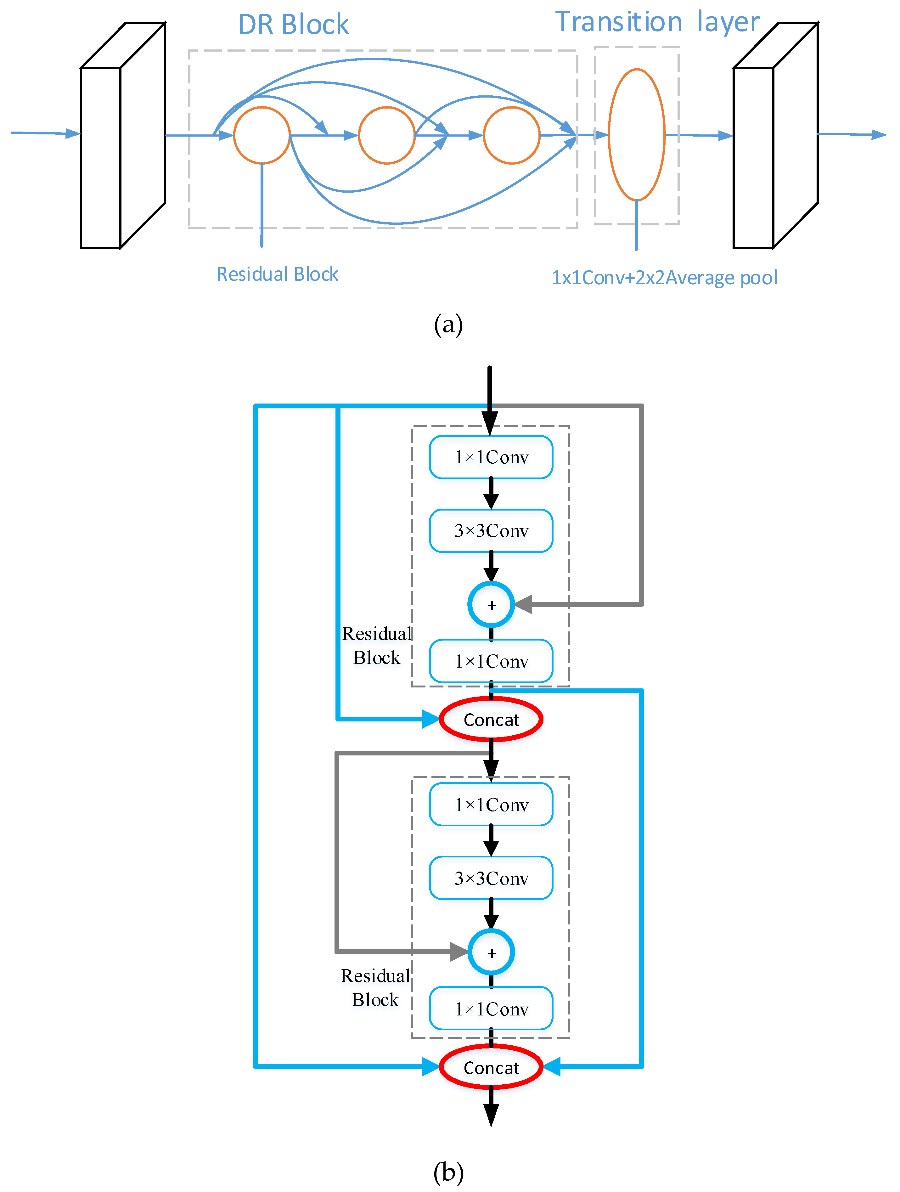
In view of the shortcomings of the original algorithm in building recognition, this paper makes the following two improvements: Firstly, this paper replaces the basic network in the original algorithm with DRNet (Dense Residual Network), which effectively utilizes the edge texture information between the target building and the backgrounds of the lower layer, realizes the repeated use of features and improves the accuracy of feature block; secondly, this paper replaces the original RoI Pooling layer with the RoI Align layer, which reduces the error caused by integer quantization and solves the problem of region mismatch in the original algorithm.

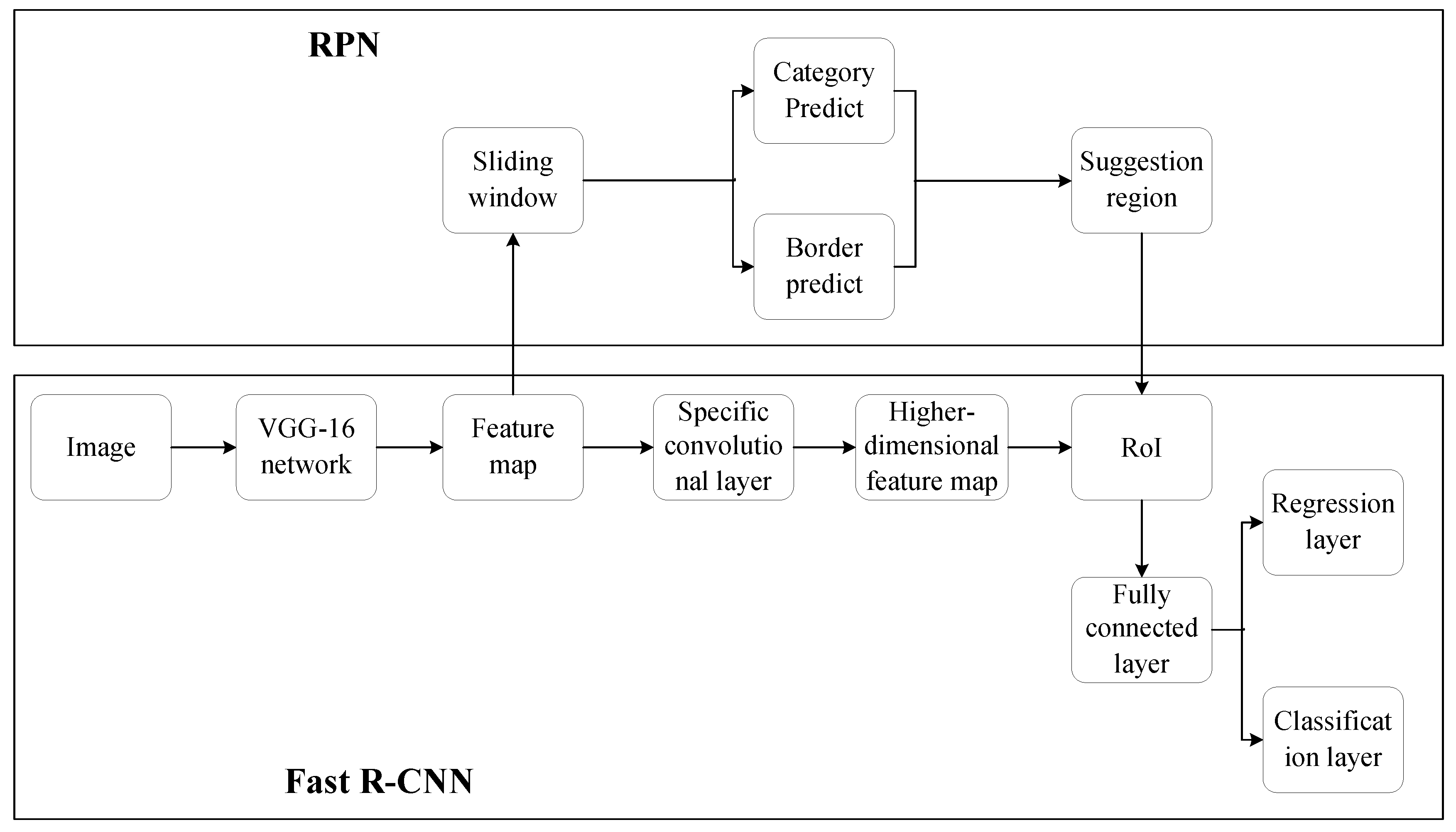
The remainder of this paper is organized as follows: Section 2 introduces the Faster R-CNN. Section 3 presents the design of the DRNet and the description of RoI Align layer. The simulations and experimental results are validated in Section 4, and the numerical results are analyzed. Finally, Section 5 concludes the paper.

2. Faster R-CNN and the Improvement Methods

2.1. Faster R-CNN

Faster R-CNN is a relatively classical deep learning algorithm, which has high recognition accuracy, efficiency and good recognition rate for the large target area [23,24]. Faster R-CNN algorithm mainly consists of two modules: the Fast R-CNN detection module and the RPN (Region Proposal Network) extraction module. The RPN is used to generate high-quality region from the basic feature map, and the Fast R-CNN directly detects and identifies the targets in the extracted suggestions region.

Figure 1 shows the processing diagram of Faster R-CNN. Firstly, the images of any size were put into the VGG-16 (Visual Geometry Group network with 16-layer) network. Secondly, the CNN network generated the shared convolutional layer and obtained the feature map. On the one hand, the feature map was put into the RPN network; on the other hand, it propagated further to the specific convolutional layer and generated the higher-dimensional feature map. Thirdly, the higher-dimensional feature map and the suggestion region was put into the RoI Pooling, and the features of the suggestion region were extracted. Then, the features were entered into the following regression layer and classification layer. The NMS (Non-Maximum Suppression) algorithm was used to remove similar results from the predicted target [25]. Finally, the algorithm gave the object category of target and the coordinates of the region.

The Faster R-CNN algorithm has achieved excellent results in the field of target detection and recognition, and the performance of deep learning has been greatly improved. However, the faster R-CNN algorithm is still lacking in some respects. Along with the network, the edge texture information of the lower layer is filtered out slowly in the convolution process, and the feature maps of the network in the extraction are not particularly accurate. However, the edge texture information of the building is particularly important in the recognition for the building distinguish from other categories of buildings. At the same time, the candidate boxes are quantized twice in the RoI Pooling. There is a problem of mismatch between the actual candidate boxes and the obtained candidate boxes.

2.2. Some Improvement Methods of RPN

When a UAV (Unmanned Aerial Vehicles) takes images, it is likely to be affected by the weather or light, and the structure of the fuzzy edge information in the environment may also be affected by the shooting angle. Therefore, the characteristics of the structure present in the images are different from the characteristics of the real one. It is possible to misidentify these particular images if the feature extraction ability of network is limited. Therefore, the extraction method affects the final result of the building detection.

The original RPN network adopts the output of a conv5_3 layer (the third convolution layer inside the fifth convolution block of VGG16) as the feature block, which is only related to the output of the previous one layer of convolution network, and has less to do with the output of the other previous layers. As a result, as the number of layers increases, and the amount of available feature information becomes increasingly smaller. It is possible that the accuracy of the network has reached saturation, and the subsequent addition of layers to the network is redundant. Therefore, the identification of buildings requires a deeper basic network to learn more feature information. In CVPR2016 (2016 IEEE Conference on Computer Vision and Pattern Recognition), the proposed ResNet model solves the problem that the deep convolutional neural network model is difficult to train and allows the number of layers of neural network to continue to increase. ResNet protects the integrity of information by directly passing the input information to the output, and the whole network only needs to learn the part of the difference between input and output, thus simplifying the difficulty of network learning. ResNet solves the degradation of deep networks through residual learning and allows training deeper networks.

With the deepening of the network, the feature information contained in the feature diagram that can be extracted is more abundant. However, for building image recognition, there is a lot of texture information at the edge of the building, which is very important for recognition. This feature information will be lost in the convolution process using the original network. DenseNet is a way to solve this problem, which makes the feature information generated in the feature diagram more abundant, and thus, the original feature information can be used.

3. Proposed Optimized Method for Faster R-CNN

3.1. DRNet

Although DenseNet can reuse the feature information of the previous layers and has a good effect on the training set, the recognition effect of the network is not greatly improved during the test set. In the DenseNet, the output of the previous dense block which connected with all the input of the previous dense blocks on the channel dimension is the input of the present dense block. Thus, the feature information of the previous layers will be reused. However, each dense block is fixed to 32 feature diagrams, and the feature information of the present dense block is decreased due to the number of previous dense blocks increasing, which will lead to degradation of the network.

Therefore, this paper proposes a DRNet, which adopts the residual blocks to replace the dense blocks. Meanwhile, the feature reuse of DenseNet is retained. As shown in Figure 2, each DR block consists of multiple residual blocks through a dense connection, and each residual block is composed of two convolutions of 1 × 1 and one convolution of 3 × 3. The two convolutions of 1 × 1 at the front and rear ends are used to reduce the feature dimension and the calculation amount of the model. Compared to the DenseNet, only the convolution of 3 × 3 in the middle is weighted in DRNet. Figure 2b shows the DR block; the output of the residual block will connect with all the input of the previous residual blocks on the channel dimension, and the result will be the input of the next residual block, so that the feature information of the previous layers will be reused in the following network. The final output is the concatenation of the output of the last residual block and all the input of the residual blocks. As with the DenseNet, the transition layer is used to reduce the dimension of the feature diagram and reduce the complexity of the network before the final output is sent to the next layer of the network.

The equation for DRNet is shown below:

$$x_l=D_l\left(\left[x_1,x_2,\dots ,x_{l-1},x_{l-1}+F_{l-1}(x_{l-1})\right]\right)$$

(1)

$$x_{l-1}=D_{l-1}\left(\left[x_1,x_2,\dots ,x_{l-2},x_{l-2}+F_{l-2}(x_{l-2})\right]\right)$$

(2)

where x_l is the input of lth residual blocks, $x_l+F_l(x_l)$ is the result of the lth residual block, and D_l is the concat process.

The convolution operation required in each DR block is more than that in the dense block. DRNet preserves the feature reuse of the network by densely connecting each residual block and prevents network degradation by the concat process of previous residual blocks. Although each block becomes more complex, the network structure of the model is simplified, and the number of feature Diagrams that can be learned by each DR block is increased.

The processed image of buildings was put into the convolutional neural network for feature extraction. The size of the image in the data set is not fixed, and it is assumed that the size of the input image is 256 × 256. The basic network structure of the improved DRNet is shown in

Table 1. DRNet basic network.

Layers	Output Size	Structure
Conv (Convolution)	$256\times 256,32$	7 × 7conv, stride2
Pooling	$128\times 128,64$	3 × 3max pool, stride2
DR block	$128\times 128,64$	$\left[\begin{array}{c}1\times 1\mathrm{conv}\\ 3\times 3\mathrm{conv}\\ 1\times 1\mathrm{conv}\end{array}\right]\times 4$
Transition Layer	$128\times 128,128$	1×1conv
	$64\times 64,128$	2 × 2average pool, stride2
DR block	$64\times 64,64$	$\left[\begin{array}{c}1\times 1\mathrm{conv}\\ 3\times 3\mathrm{conv}\\ 1\times 1\mathrm{conv}\end{array}\right]\times 8$
Transition Layer	$64\times 64,256$	1×1conv
	$32\times 32,256$	2 × 2average pool, stride2
DR block	$32\times 32,64$	$\left[\begin{array}{c}1\times 1\mathrm{conv}\\ 3\times 3\mathrm{conv}\\ 1\times 1\mathrm{conv}\end{array}\right]\times 16$
Transition Layer	$32\times 32,512$	1×1conv
	$16\times 16,512$	2 × 2average pool, stride2

. First, the processed image was put into a 7 × 7 convolution layer, whose stride is 2. The feature diagram obtained by a large convolution kernel can obtain a larger receptive field and provide more feature information for the subsequent layer. Secondly, the result was entered into a 3 × 3 maximum pool. The pooling layer, whose stride is 2, will halve the length and width of the feature diagram, retain the main feature information, and reduce the calculation amount of the next layer. Then, three DR blocks and transition layers are passed successively. Each DR block was composed of continuously connected convolutional layers of 1 × 1 and 3 × 3. Each small block outputs the feature diagram of 64 channels, which is then superimposed in turn and becomes the input of the next small block to realize the reuse of feature information. The transition layer consists of a 1 × 1 convolution layer and a 2 × 2 average pool layer whose stride is 2. While the DR block enriches the feature information of the feature diagram, the transition layer reduces the size of feature diagram and reduces the computation of model. Finally, the feature diagram of c × 512 × 16 × 16 output by the model was used as the input of the RPN module to further extract the candidate diagram and make the category prediction, and at the same time, it was used as the mapping feature diagram of the RoI layer to keep it consistent with the original algorithm.

3.2. Description of RoI Layer

RoI refers to the candidate block on the feature diagram. In the faster R-CNN algorithm, candidate blocks are generated through RPN, and then, these candidate blocks are mapped on the feature diagram to get RoI.

The candidate box for faster R-CNN is obtained by border prediction, but most of the coordinates are floating point numbers, and they are quantized as integer coordinates for calculation. Then, the candidate box is divided evenly, and the boundaries of each divided unit are integers. Therefore, as shown in Figure 3, the integer for RoI Pooling consists of two processes. In fact, after these processes, the candidate box obtained has a certain deviation from the original position returned from RPN, which will affect the accuracy of detection or segmentation.

To solve this problem, the RoI Align [26] method was used to cancel the integer operation and keep the floating point number. In the RoI Align method, the bilinear interpolation method is used to obtain the image value on the pixel point whose coordinate is a floating point number, so that the mapping of RoI is more accurate.

Bilinear interpolation is essentially linear interpolation in two directions. The image amplified by the bilinear interpolation algorithm is of high quality and there will be no discontinuous pixel values. As shown in Figure 4, in the x direction, the algorithm first interpolates linearly between Q₁₁ and Q₂₁ to get R₁ and R₂ and then interpolates linearly between R₁ and R₂ in the y direction to get the final point P.

In the x direction, R1 and R2 can be obtained from Equations (3) and (4):

$$f\left(R_1\right)\approx \frac{x_2-x}{x_2-x_1}f\left(Q_{11}\right)+\frac{x-x_1}{x_2-x_1}f\left(Q_{21}\right) Where R_1=\left(x,y_1\right)$$

(3)

$$f\left(R_2\right)\approx \frac{x_2-x}{x_2-x_1}f\left(Q_{12}\right)+\frac{x-x_1}{x_2-x_1}f\left(Q_{22}\right) Where R_1=\left(x,y_2\right)$$

(4)

In the y direction, y can be obtained from Equation (5):

$$f\left(P\right)\approx \frac{y_2-y}{y_2-y_1}f\left(R_1\right)+\frac{y-y_1}{y_2-y_1}f\left(R_2\right)$$

(5)

f (x,y) is shown in Equation (6):

$$\begin{array}{l}f\left(x,y\right)\approx \frac{f\left(Q_{11}\right)}{\left(x_2-x_1\right)\left(y_2-y_1\right)}\left(x_2-x\right)\left(y_2-y\right)\\ +\frac{f\left(Q_{21}\right)}{\left(x_2-x_1\right)\left(y_2-y_1\right)}\left(x-x_1\right)\left(y_2-y\right)\\ +\frac{f\left(Q_{12}\right)}{\left(x_2-x_1\right)\left(y_2-y_1\right)}\left(x_2-x\right)\left(y-y_1\right)\\ +\frac{f\left(Q_{22}\right)}{\left(x_2-x_1\right)\left(y_2-y_1\right)}\left(x-x_1\right)\left(y-y_1\right)\end{array}$$

(6)

As shown in Figure 5, the dotted part represents the feature diagram and the solid line represents RoI. RoI is divided into 2 × 2 cells. If the sampling point is 4, we first divided each cell into four small squares as shown with the black line in Figure 5, with the center of each square being the sampling point. The coordinates of these sampling points were usually floating point numbers; thus, bilinear interpolation is required for the sampling pixel. Then, the pixel value was calculated: As shown by the four arrows, each corresponded to the pixel value of 1, 2, 3 and 4. Finally, the four sampling points in each cell are max-pooling and the method of RoI Align can obtain the final result.

In the relevant experiments of building remote sensing image recognition, we found that the best performance can be obtained by setting four sampling points. Moreover, if there is only one sampling point, that is, only the pixel value of the sampling point needs to be taken, the obtained performance will not be too bad. In fact, RoI Align does not have as many traversing sampling points as RoI Pooling, but it can achieve better performance, which is mainly attributed to solving the problem of area mismatch.

4. Image Acquisition and Recognition

The building data set images produced in this paper are from low-altitude remote sensing images taken by UAVs. The size of the images varies from tens to hundreds of kb. In the production of the data set, images of different weather, different illumination and different angles were collected, which adds a certain difficulty to the identification of buildings and ensures the applicability and diversity of the data set. The weather blurs the image of the building and filters out some edge information. The lighting ensures that the building can be clearly seen, and part of the characteristic information of the building will be retained at night. The angle ensures that the deformation of the building is within a certain range. For the collected data set, we adopted the same format as VOC2007 (Visual Object Classes 2007) to annotate.

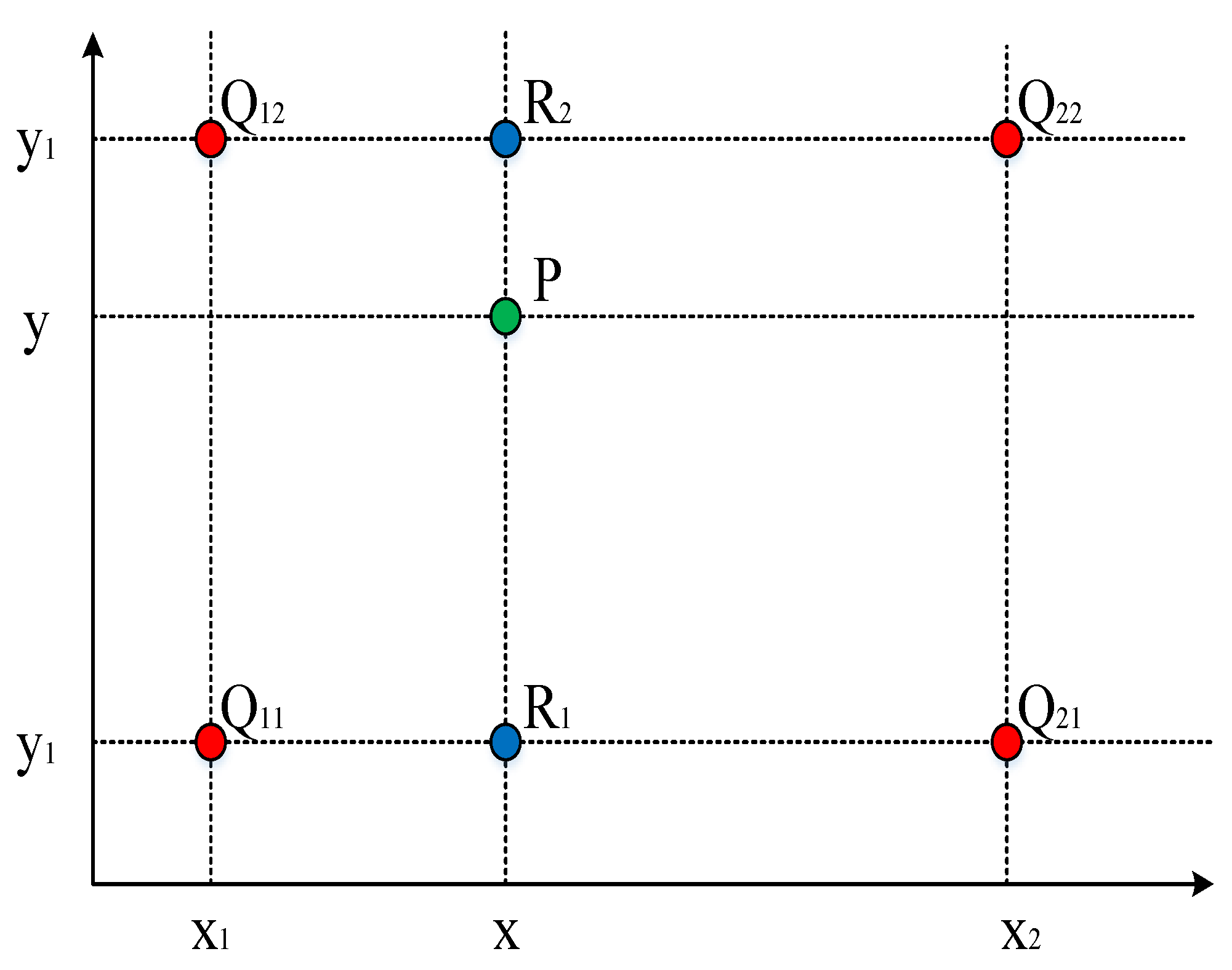
For the improved faster R-CNN algorithm, since the collected building images are all compressed, the algorithm will resize the building images when inputting the images. Then, the algorithm set the shortest side short_size = 600. If the height of the input image h is larger than the width w, the value of short_size/h = scale is the reference scale. After modification, the value of the height is h = h × scale and the value of width is w = w × scale. The advantage of this approach is that the input image is a little larger than the original image, and it has some improvement on the target of small scale due the upsampling of the images [27].

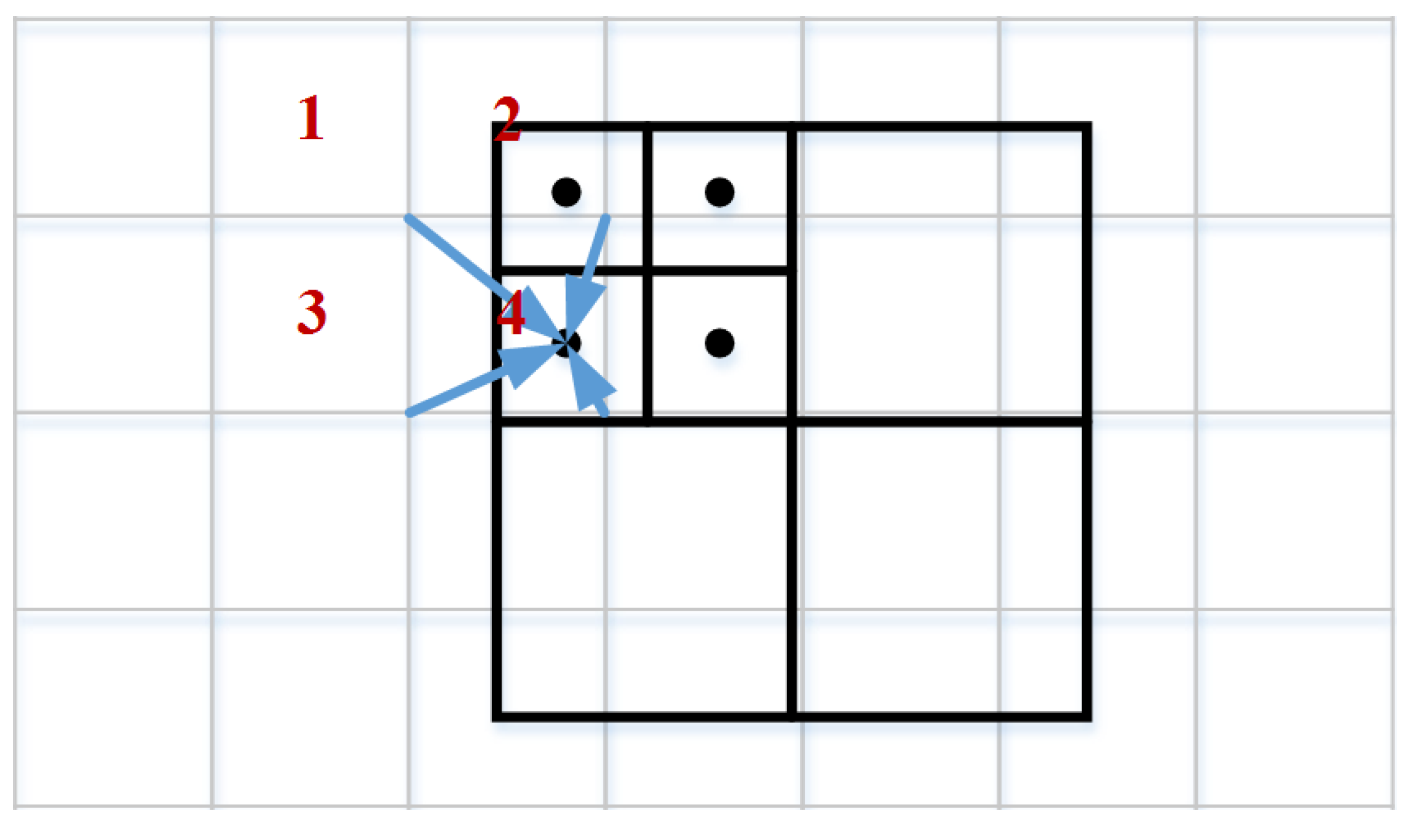
RPN does not need uniform size of the input feature diagrams; thus, the final output size of candidate diagrams is different. RPN adopts the sliding window to traverse the feature diagram, and the feature pixels on the sliding window correspond to nine kinds of anchor frames. The short side of the input image was adjusted to 600 pixels in the actual processing of the network, and then, the long side of the input image was adjusted in the same proportion. Due to the different sizes of anchor frames, the training process of the RPN can be regarded as multi-scale training in a sense. Then, the traversal result and anchor frame were sent into the full connection layer for classification and regression. The classification and regression, respectively, predict the probability and coordinates of the building in the image. In order to get a high-quality prediction box, this paper filters the redundant prediction boxes base on faster R-CNN, and compares the mark box with the boxes predicted by RPN; the proportion of the overlapped area and the union area of the two boxes is the contact ratio. The contact ratio higher than 0.7 in the image is the positive sample, which contains a clear image of the building, and the contact ratio lower than 0.3 in the image is the negative sample, which is the background image, excluding the building. The buildings and backgrounds are intermingled in the rest of the anchor box; the training model without any contribution should not be used. The rest of the anchor boxes are not being used, due to the fact that buildings and backgrounds were intermingled in the rest of the anchor boxes and they did not contribute to the model training.

The candidate diagram extracted from the RPN is sent to the RoI Align layer as input and mapped to the previously obtained feature diagram, that is, the position of the candidate diagram is marked on the feature diagram. For these candidate diagrams, 7 × 7 RoI was also adopted. However, each 1 × 1 block was no longer fixed as an integer, and the floating point number was retained, so that the candidate diagrams can be fully presented on the feature diagram. In this way, these more accurate feature diagrams will be classified by the full connection layer and softmax to get the prediction probability of buildings. Our network conducted border regression on the feature diagram again to obtain the candidate box with higher accuracy, resulting in better identification of the coordinates of building. Then, the network eliminated the cross-repetition window by non-maximum suppression algorithm, found out the best object detection position and selected the building whose prediction probability was greater than 0.6. In this way, the network could identify the building and the area in the image.

In the field of deep learning, precision and recall [28] are widely used to evaluate the quality of results. The precision rate is the ratio of the number of relevant samples retrieved to the total number of retrieved samples, which measures the accuracy of the retrieval system. Recall rate refers to the ratio between the number of relevant samples retrieved and all relevant samples in the sample database, which measures the recall rate of the retrieval system.

The precision rate is defined in terms of the predicted outcome, which means the proportion of the actually positive samples and the predicted positive samples. Therefore, there are two possibilities for the prediction of positive. One is to predict the positive samples as the positive (TP), and the other is to predict the negative samples as the positive (FP). The equation of precision rate is as follows:

$$P=\frac{TP}{TP+FP}$$

(7)

The recall rate is for our original sample, which means how many positive samples were predicted correctly. There are also two possibilities. One is to predict the original positive samples to be positive (TN), and the other is to predict the original positive samples to be negative (FN). The equation of the recall rate is as follows:

$$R=\frac{TN}{TN+FN}$$

(8)

The precision-recall (PR) curve is a performance judgment for the models of building detection. It can be judged by comparing the average precision (AP). The AP represents the area under the PR curve. The larger the area, the better the model performance. If we want to determine the performance for all types of the buildings, we can calculate the mean average precision (mAP) for all types of buildings.

In this paper, the remote sensing image contains the target building, and the background outside the target building. Therefore, the target buildings are the positive samples and the backgrounds are the negative samples. In the experiment, the deep learning framework MXNet developed by Amazon was used as the software testing platform. It provides C++ and Python interfaces, and has as important features fast speed, memory saving and high parallel efficiency. The 64-bit Ubuntu18.04.2 LTs operating system was adopted as the test environment and the video card GeForce GTX1080ti 8G video memory was configured. During the training, the model trained 100 epochs of the training set; each Epoch completed one training of the training set, the initial learning rate of the model was set as 0.001 and the learning rate decreased by 10% every 15 epochs.

This paper improved the base network and RoI layer of Faster R-CNN algorithm for building recognition. Therefore, this chapter tests the model from these two points respectively.

Different basic networks improve the performance of the model differently. In order to verify the advantages of DRNet in feature extraction, the paper, respectively, used ResNet, DenseNet and DRNet as the basic network of Faster R-CNN for testing in this section. In order to reduce the influence of other factors, the model was trained with the same experimental data set, iterations and training parameters, completed on the same hardware platform and experimental environment. In the RoI layer, the RoI Pooling was used in this section to extract the feature diagram of a fixed size.

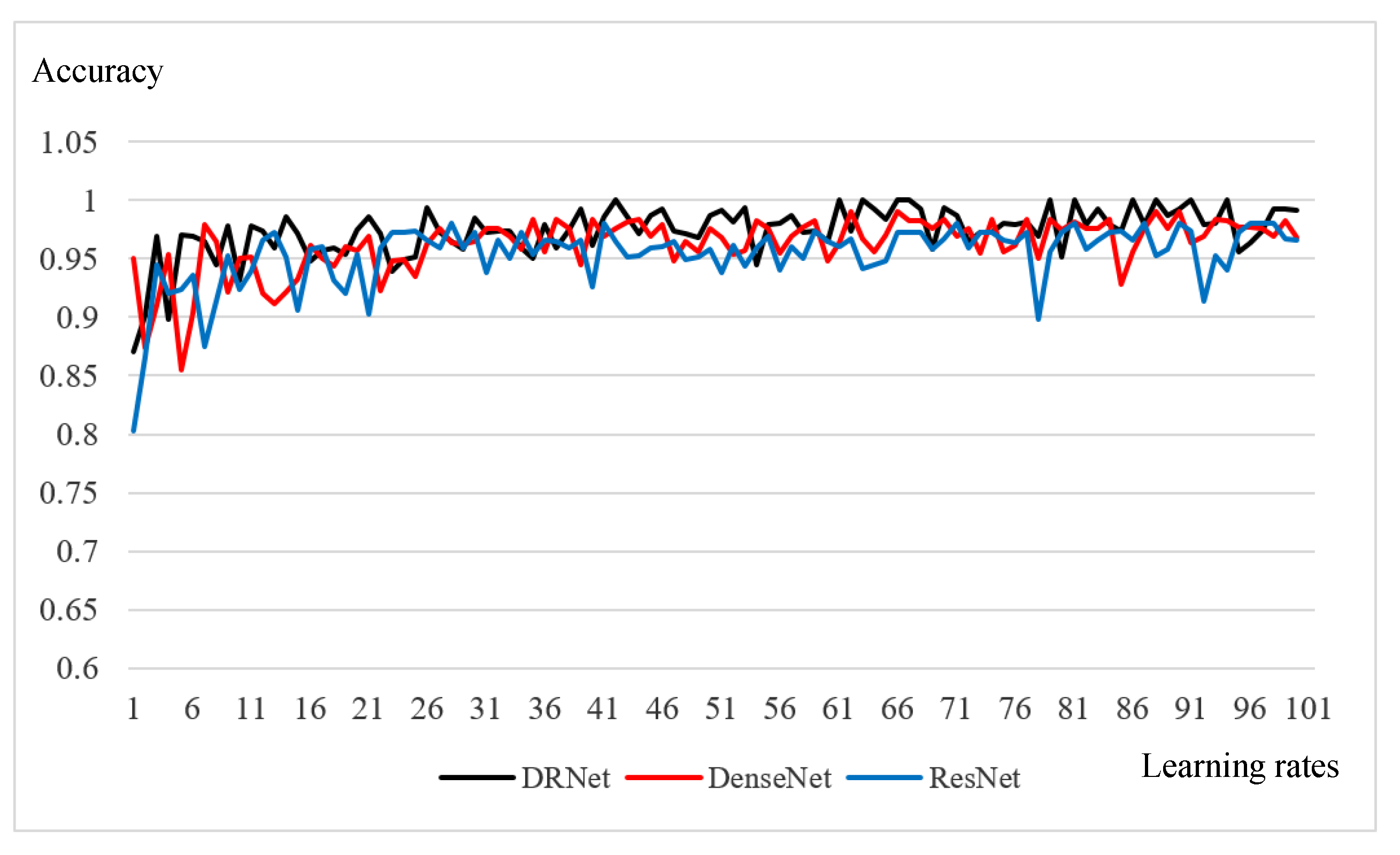
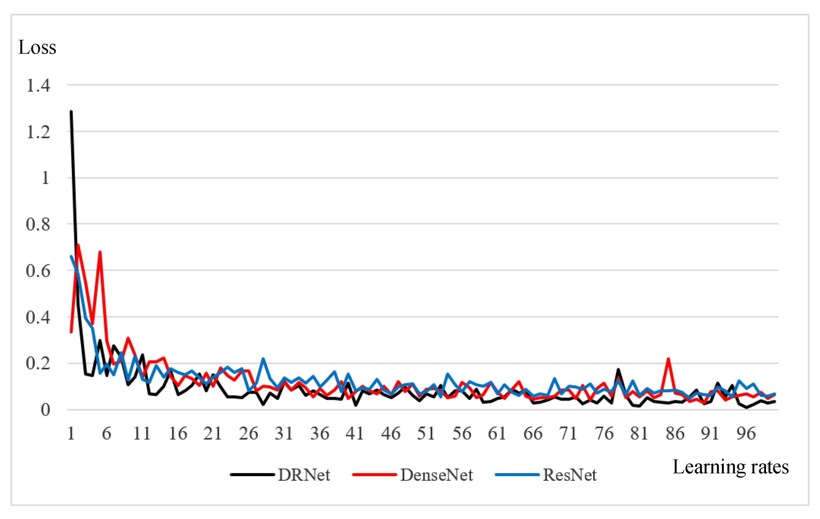
During the training, the training time of an Epoch was approximately 580.8 s for DRNet, 557.8 s for DenseNet and 517.6 s for ResNet. Although the DRNet network was relatively complex, the training time did not increase much. After the training, the accuracy curve of the three networks is shown in Figure 6. Obviously, the model using DRNet as the basic network has a higher accuracy, slightly better than the other two models, and with the decrease of learning rate, the image disturbance is small. The loss curve of the three networks is shown in Figure 7. Using the DRNet network model, the loss fell faster than it did in the other two models, and the final loss value was slightly less than the other two models; thus, the training effect of DRNet model is better.

The same test set was used to test the three basic network models, and an example of a PR curve for Potala Palace in Lhasa is shown in Figure 8. As shown in the PR curve, the building detection performances of three basic network models are acceptable, but it is hard to evaluate which model is better from the curve. Therefore, this paper adopted mAP to evaluate the performances of the three models for different buildings.

As the results in

Table 2. Experiment results depend on different basic network.

Basic Network	mAP (%)	Time (s)
ResNet	76.8	1.15
DenseNet	78.0	1.28
DRNet	81.8	1.52

show, the mAP value of the ResNet network is the lowest, only 76.8%, indicating that although this network solves the problem of network degradation and increases the number of network layers, the recognition effect of building images is a little behind. The mAP of the DenseNet model was improved by 1.2% compared with ResNet, because DenseNet can make the high-level network reuse the characteristic information of the low-level network, and the network model becomes more complex. The DRNet network designed in this paper can not only be repeated for low-level feature information, but each DR block can extract more feature information and prevent network degradation; the mAP is increased by 3.8% compared with DenseNet. Obviously, the stronger the ability of the basic network to extract the characteristic information of the building, the better the performance of the model; the basic network of DRNet showed the best ability to extract building features in this paper. As the layer number of network model increases and the network becomes more and more complex, the amount of computation increases, and it takes more time to identify a building; however, the recognition effect is getting better. Additionally, with the improvement of computer performance, this will no longer be a problem.

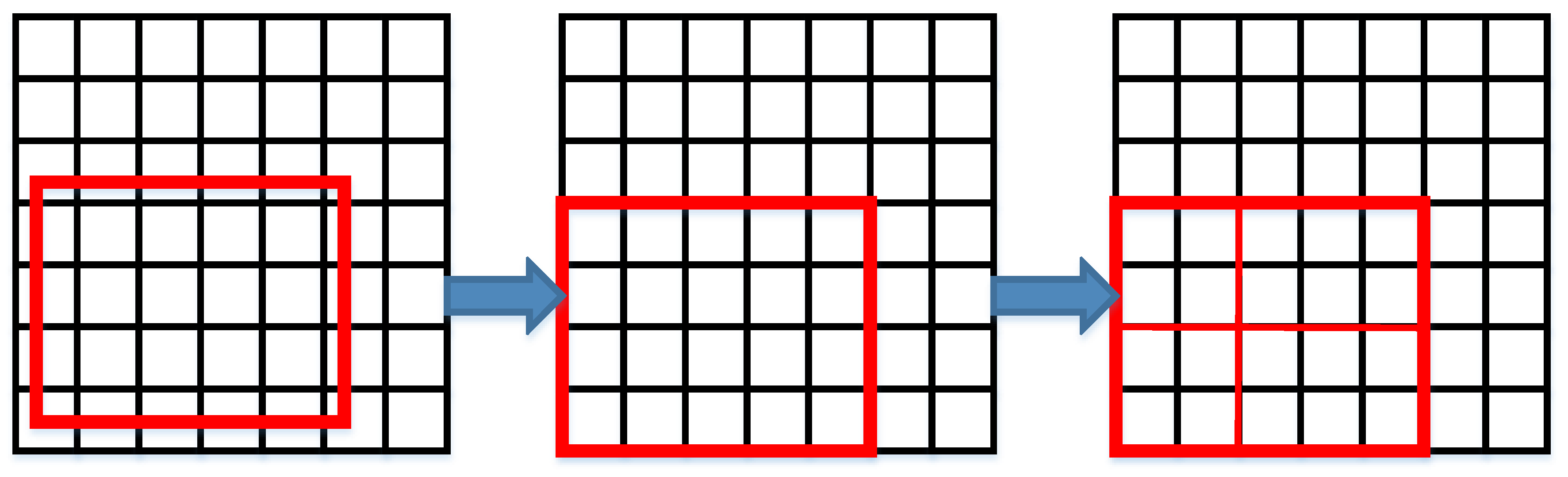
The size of the building images is not fixed in the data set. If the size of the image cannot be divisible by 16, integer quantization will be done when the RoI Pooling layer carries out feature mapping of the candidate box with fixed size, and there will be some errors between the output feature diagram and the actual feature diagram. The RoI Align layer used in this paper accurately divides the candidate diagram through bilinear difference method. Even if the image size cannot be divided by 16, an RoI Align layer will retain the floating point coordinates of these fixed size feature maps, which solves the problem of region mismatch. In this section, DRNet is used as the base network of faster R-CNN model, and other training configurations are consistent with the above section. The RoI Pooling layer and RoI Align layer are, respectively, used as the RoI layer of the original model for the experiments. After the training, the same test set was used to detect these two RoI layers, respectively, and the results are shown in

Table 3. Experiment results depend on different RoI layers.

RoI Layers	mAP (%)	Time (s)
RoI Pooling	81.8	1.52
RoI Align	82.1	1.54

.

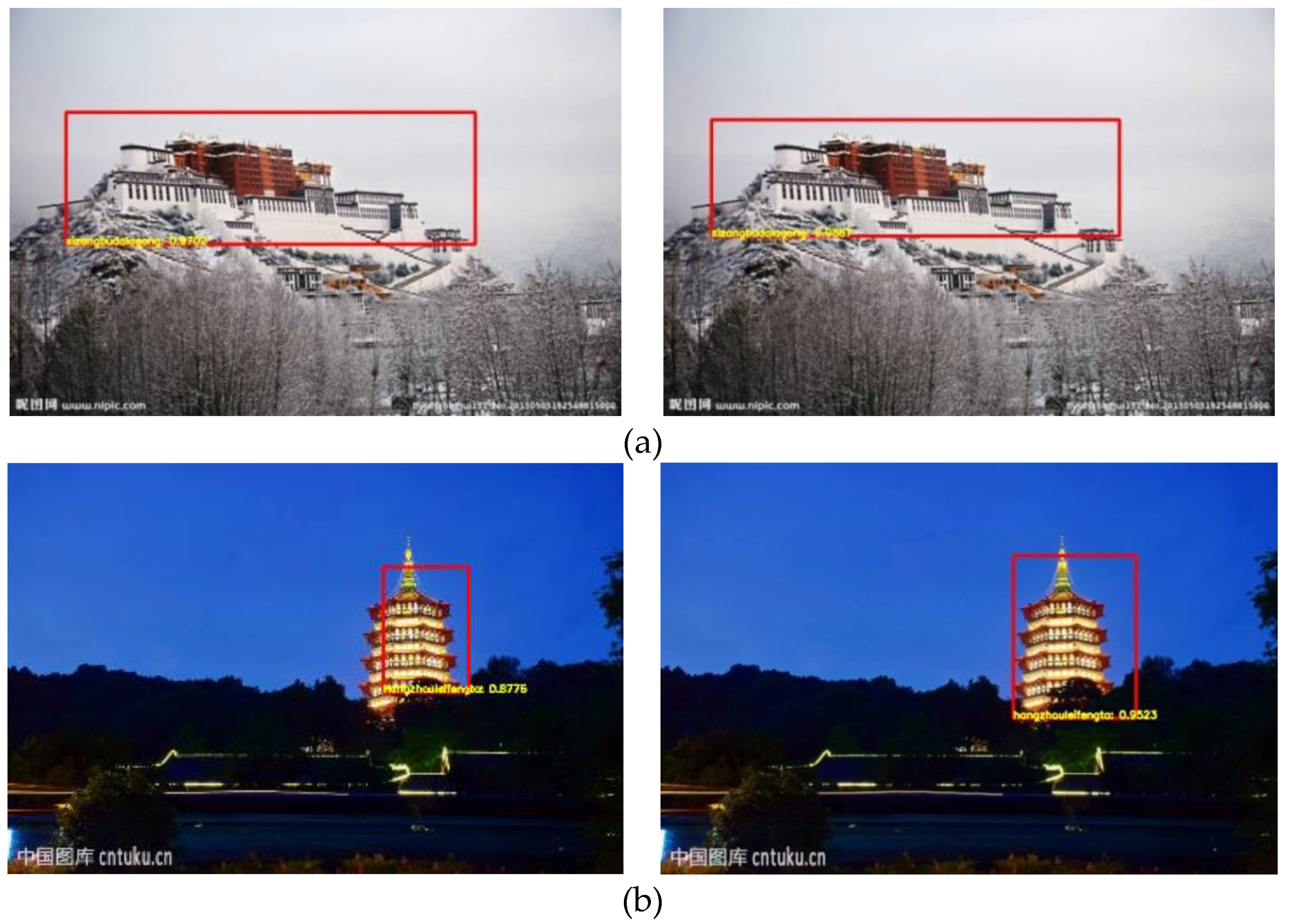
Experimental results in Table 3 show that the mAP value using the RoI Pooling layer model is lower than with RoI Align. This is because the RoI Pooling layer of two integers quantitative caused an area mismatch problem, and RoI Align has some improvement on this problem The mAP values have a 0.3% improvement, so that the recognition effect of using the RoI Align layer is better for the building data sets without fixed size in this paper. Moreover, the number of network layers has not changed, and the recognition time of an image has hardly changed. Part of the test images is shown in Figure 9.

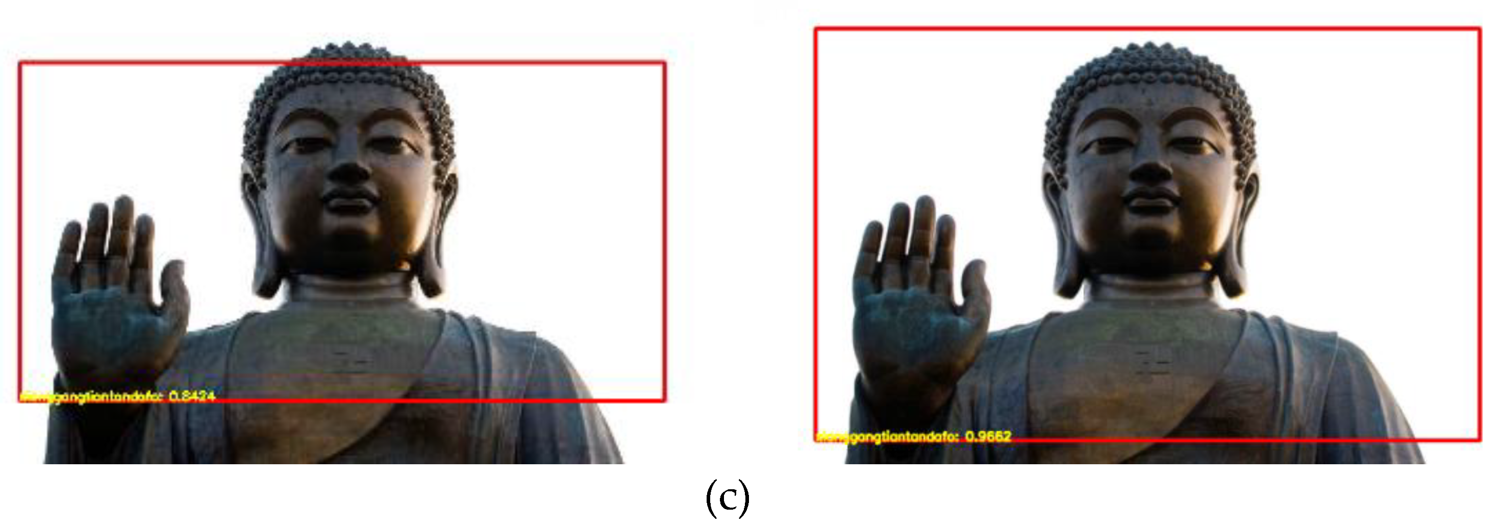
The left column shows the test result using the RoI Pooling layer, and the right column shows the test result using RoI Align. The model using the RoI Align layer can predict the area of buildings in the image more accurately and in a wider range, and the target buildings are basically in the predicted area. Due to the problem of area mismatch, the prediction of the target building using the RoI Pooling layer has a large deviation, and only part of the target building was included in the prediction box. This also caused the different results of the building detection; the similarity results with the real building in the data set are shown in

Table 4. Building detection results depend on different RoI layers.

Similarity with the Real Building of Different RoI Layers	Potala Palace in Lhasa	Leifeng Pagoda in Hangzhou	Giant Buddha at the Temple of Heaven in Hong Kong
RoI Pooling (%)	97.02	87.76	84.24
RoI Align (%)	98.57	95.23	96.96

. The RoI Align layer showed great improvement for the last two buildings, namely, 7.47% and 12.72%, respectively.

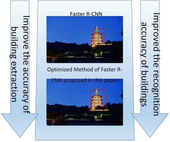
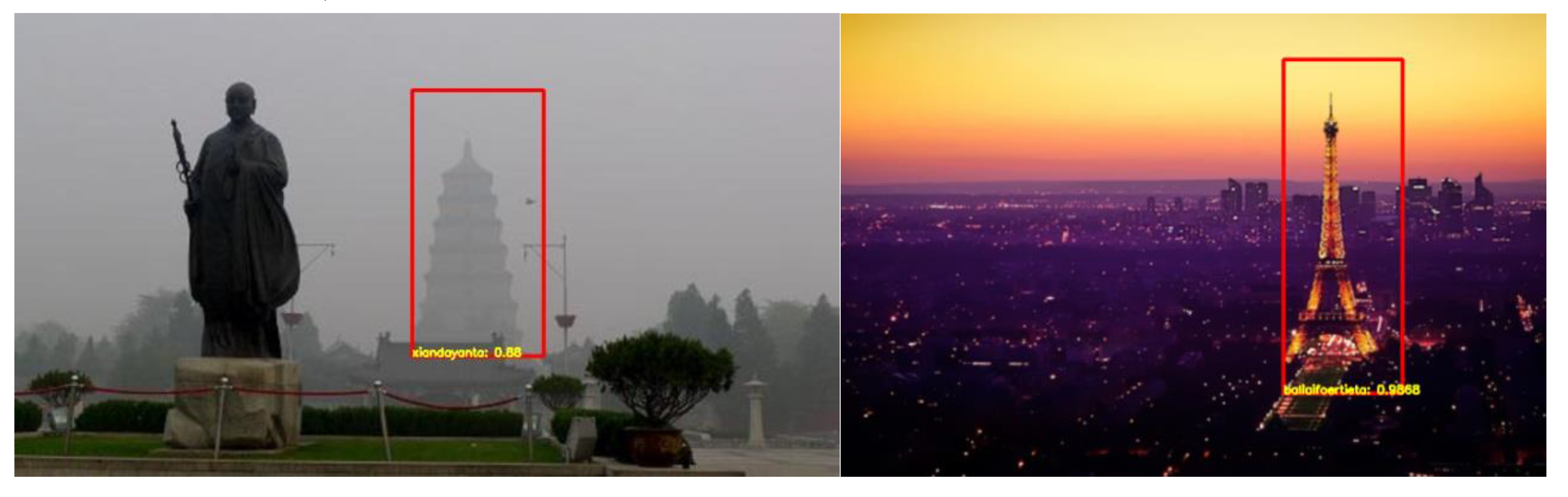
At the same time, the RoI Align layer model also has a good recognition effect on buildings in complex environments (in fog weather or at night) that are difficult to be recognized by the original model, as shown in Figure 10.

5. Conclusions

In the remote sensing recognition of buildings, most buildings are often in a complex background, so that the edge information of buildings is often covered by these backgrounds. However, the traditional faster R-CNN algorithm is less efficient in identifying small targets with complex backgrounds, and the identified building differ greatly from the real targets. This paper improves the faster R-CNN algorithm with the DRNet method, which is a residual block network with dense connections base on the basic network. DRNet not only alleviates the problem of gradient disappearance and deepens the depth of the network model but also strengthens the reuse of the feature information of the lower layer network. In the complex environment, more feature information can be extracted, and the buildings finally identified are more accurate. Moreover, the RoI Align bilinear interpolation method was used in the RoI layer to reduce the error caused by the integer quantization of the original RoI Pooling layer, solve the problem of region mismatch and make the extracted candidate diagram more accurate and closer to the real target.

References

1. Zhu, X.X.; Tuia, D.; Mou, L.; Xia, G.-S.; Zhang, L.; Xu, F.; Fraundorfer, F. Deep Learning in Remote Sensing: A Comprehensive Review and List of Resources. IEEE Geosci. Remote Sens. Mag. 2017, 5, 8–36. [Google Scholar] [CrossRef] [Green Version]
2. Pandit, V.R.; Bhiwani, R.J. Image Fusion in Remote Sensing Applications: A Review. Int. J. Comput. Appl. 2015, 120, 22–32. [Google Scholar]
3. Lecun, Y. Deep learning & convolutional networks. In Proceedings of the IEEE Hot Chips Symposium, Cupertino, CA, USA, 23–25 August 2015. [Google Scholar]
4. LeCun, Y.; Bottou, L.; Bengio, Y.; Haffner, P. Gradient-based learning applied to document recognition. Proc. IEEE 1998, 86, 2278–2324. [Google Scholar]
5. Hinton, G.E.; Osindero, S.; Teh, Y.-W. A Fast Learning Algorithm for Deep Belief Nets. Neural Comput. 2006, 18, 1527–1554. [Google Scholar] [CrossRef] [PubMed]
6. Lawrence, S.; Giles, C. Overfitting and neural networks: Conjugate gradient and backpropagation. In Proceedings of the IEEE-INNS-ENNS International Joint Conference on Neural Networks. IJCNN 2000. Neural Computing: New Challenges and Perspectives for the New Millennium, Como, Italy, 27 July 2000; Institute of Electrical and Electronics Engineers (IEEE), 2000. [Google Scholar]
7. Krizhevsky, A.; Sutskever, I.; Hinton, G.E. Pdf ImageNet classification with deep convolutional neural networks. Commun. ACM 2017, 60, 84–90. [Google Scholar] [CrossRef]
8. Simonyan, K.; Zisserman, A. Very deep convolutional networks for large-scale image recognition. arXiv 2014, arXiv:1409.1556. [Google Scholar]
9. Szegedy, C.; Liu, W.; Jia, Y.; Sermanet, P.; Reed, S.; Anguelov, D.; Erhan, D.; Vanhoucke, V.; Rabinovich, A. Going deeper with convolutions. In Proceedings of the 2015 IEEE Conference on Computer Vision and Pattern Recognition (CVPR), Boston, MA, USA, 7–12 June 2015; Institute of Electrical and Electronics Engineers (IEEE), 2015; pp. 1–9. [Google Scholar]
10. He, K.; Zhang, X.; Ren, S.; Sun, J. Deep Residual Learning for Image Recognition. In Proceedings of the 2016 IEEE Conference on Computer Vision and Pattern Recognition (CVPR), Las Vegas, NV, USA, 27–30 June 2016; Institute of Electrical and Electronics Engineers (IEEE), 2016; pp. 770–778. [Google Scholar]
11. Huang, G.; Liu, Z.; Van Der Maaten, L.; Weinberger, K.Q. Densely Connected Convolutional Networks. In Proceedings of the 2017 IEEE Conference on Computer Vision and Pattern Recognition (CVPR), Honolulu, HI, USA, 21–26 July 2017; Institute of Electrical and Electronics Engineers (IEEE), 2017; pp. 2261–2269. [Google Scholar]
12. Zeiler, M.D.; Fergus, R. Visualizing and Understanding Convolutional Networks. In Proceedings of the European Conference on Computer Vision, Zurich, Switzerland, 6–12 September 2014. [Google Scholar]
13. Ma, C.; Huang, J.-B.; Yang, X.; Yang, M.-H. Hierarchical Convolutional Features for Visual Tracking. In Proceedings of the 2015 IEEE International Conference on Computer Vision (ICCV), Boston, MA, USA, 7–12 June 2015; Institute of Electrical and Electronics Engineers (IEEE), 2015; pp. 3074–3082. [Google Scholar]
14. Cinbis, R.G.; Verbeek, J.; Schmid, C. Weakly Supervised Object Localization with Multi-Fold Multiple Instance Learning. IEEE Trans. Pattern Anal. Mach. Intell. 2016, 39, 189–203. [Google Scholar] [CrossRef] [PubMed]
15. Dai, J.; Li, Y.; He, K.; Sun, J. R-fcn: Object detection via region-based fully convolutional networks. In Proceedings of the Neural Information Processing Systems Conference, Barcelona, Spain, 5–10 December 2016; pp. 379–387. [Google Scholar]
16. Bell, S.; Zitnick, C.L.; Bala, K.; Girshick, R. Inside-Outside Net: Detecting Objects in Context with Skip Pooling and Recurrent Neural Networks. In Proceedings of the 2016 IEEE Conference on Computer Vision and Pattern Recognition (CVPR), Las Vegas, NV, USA, 27–30 June 2016; Institute of Electrical and Electronics Engineers (IEEE), 2016; pp. 2874–2883. [Google Scholar]
17. Zhang, S.; Wen, L.; Bian, X.; Lei, Z.; Li, S.Z. Single-Shot Refinement Neural Network for Object Detection. In Proceedings of the 2018 IEEE/CVF Conference on Computer Vision and Pattern Recognition, Salt Lake City, UT, USA, 19–21 June 2018; Institute of Electrical and Electronics Engineers (IEEE), 2018; pp. 4203–4212. [Google Scholar]
18. Wang, X.; Shrivastava, A.; Gupta, A. A-Fast-RCNN: Hard Positive Generation via Adversary for Object Detection. In Proceedings of the 2017 IEEE Conference on Computer Vision and Pattern Recognition (CVPR), Honolulu, HI, USA, 21–26 July 2017; Institute of Electrical and Electronics Engineers (IEEE), 2017; pp. 3039–3048. [Google Scholar]
19. Irvin, R.; McKeown, D. Methods for exploiting the relationship between buildings and their shadows in aerial imagery. IEEE Trans. Syst. Man Cybern. 1989, 19, 1564–1575. [Google Scholar] [CrossRef] [Green Version]
20. Liow, Y.-T.; Pavlidis, T. Use of shadows for extracting buildings in aerial images. Structural Pattern Analysis, 2nd ed.; Mohr, R., Pavlidis, T., Sanfeliu, A., Eds.; World Scientific: Singapore, 1990; pp. 165–180. [Google Scholar]
21. Stassopoulou, A.; Caelli, T.; Ramirez, R. Automatic extraction of building statistics from digital orthophotos. Int. J. Geogr. Inf. Sci. 2000, 14, 795–814. [Google Scholar] [CrossRef]
22. Katartzis, A.; Sahli, H.; Nyssen, E.; Cornelis, J. Detection of buildings from a single airborne image using a Markov random field model. In Proceedings of the IGARSS 2001. Scanning the Present and Resolving the Future. IEEE 2001 International Geoscience and Remote Sensing Symposium (Cat. No.01CH37217), Sydney, Australia, 9–13 July 2001; Institute of Electrical and Electronics Engineers (IEEE), 2002; Volume 6, pp. 2832–2834. [Google Scholar]
23. Girshick, R.; Donahue, J.; Darrell, T.; Malik, J.; Malik, J. Rich Feature Hierarchies for Accurate Object Detection and Semantic Segmentation. In Proceedings of the 2014 IEEE Conference on Computer Vision and Pattern Recognition, Columbus, OH, USA, 23–28 June 2014; Institute of Electrical and Electronics Engineers (IEEE), 2014; pp. 580–587. [Google Scholar]
24. Ren, S.; He, K.; Girshick, R.; Sun, J. Faster r-cnn: Towards real-time object detection with region proposal networks. In Proceedings of the Neural Information Processing Systems Conference, Montreal, QC, Canada, 7–12 December 2015. [Google Scholar]
25. Neubeck, A.; Van Gool, L. Efficient Non-Maximum Suppression. In Proceedings of the 18th International Conference on Pattern Recognition (ICPR’06), Hong Kong, China, 20–24 August 2006; Institute of Electrical and Electronics Engineers (IEEE), 2006; Volume 3, pp. 850–855. [Google Scholar]
26. He, K.; Gkioxari, G.; Dollar, P.; Girshick, R. Mask R-CNN. IEEE Trans. Pattern Anal. Mach. Intell. 2020, 42, 386–397. [Google Scholar] [CrossRef] [PubMed]
27. Singh, B.; Davis, L.S. An Analysis of Scale Invariance in Object Detection—SNIP. In Proceedings of the 2018 IEEE/CVF Conference on Computer Vision and Pattern Recognition, Salt Lake City, UT, USA, 19–21 June 2018; Institute of Electrical and Electronics Engineers (IEEE), 2018; pp. 3578–3587. [Google Scholar]
28. Buckland, M.; Gey, F. The relationship between Recall and Precision. J. Am. Soc. Inf. Sci. 1994, 45, 12–19. [Google Scholar] [CrossRef]
Figure 1. Faster region-based Convolutional Neural Network (R-CNN).
Remotesensing 12 00762 g001
Figure 2. Schematic of a Dense Residual Network (DRNet).
Remotesensing 12 00762 g002
Figure 3. The integer processing of Region of Interest (RoI) Pooling.
Remotesensing 12 00762 g003
Figure 4. Bilinear interpolation.
Remotesensing 12 00762 g004
Figure 5. RoI Align.
Remotesensing 12 00762 g005
Figure 6. Accuracy curve of the networks.
Remotesensing 12 00762 g006
Figure 7. Loss curve of the networks.
Remotesensing 12 00762 g007
Figure 8. Precision–recall (PR) curve for Potala Palace in Lhasa.
Remotesensing 12 00762 g008
Figure 9. Experiment results of the test images. (a) Potala Palace in Lhasa. (b) Leifeng Pagoda in Hangzhou. (c) Giant Buddha at the temple of heaven in Hong Kong.
Remotesensing 12 00762 g009aRemotesensing 12 00762 g009b
Figure 10. Test images in complex environments.
Remotesensing 12 00762 g010