Article

Deep Learning-Based Drivers Emotion Classification System in Time Series Data for Remote Applications

1
Department of Unmanned Vehicle Engineering, Sejong University, 209, Neungdong-ro, Gwangjin-gu, Seoul 05006, Korea
2
Division of Electronics and Electrical Engineering, Dongguk University, 30 Pildong-ro 1-gil, Jung-gu, Seoul 100-715, Korea
3
Department of Computer Science and Engineering, Kyungpook National University, Daegu 41566, Korea
4
College of Internet of Things Engineering, Hohai University, Changzhou 213022, China
5
Department of Software, Gachon University, 1342 Seongnamdaero, Sujeong-gu, Seongnam, Gyeonggi-do 13120, Korea
*
Author to whom correspondence should be addressed.
Remote Sens. 2020, 12(3), 587; https://doi.org/10.3390/rs12030587
Submission received: 2 January 2020 / Revised: 6 February 2020 / Accepted: 6 February 2020 / Published: 10 February 2020

Abstract

:
Aggressive driving emotions is indeed one of the major causes for traffic accidents throughout the world. Real-time classification in time series data of abnormal and normal driving is a keystone to avoiding road accidents. Existing work on driving behaviors in time series data have some limitations and discomforts for the users that need to be addressed. We proposed a multimodal based method to remotely detect driver aggressiveness in order to deal these issues. The proposed method is based on change in gaze and facial emotions of drivers while driving using near-infrared (NIR) camera sensors and an illuminator installed in vehicle. Driver’s aggressive and normal time series data are collected while playing car racing and truck driving computer games, respectively, while using driving game simulator. Dlib program is used to obtain driver’s image data to extract face, left and right eye images for finding change in gaze based on convolutional neural network (CNN). Similarly, facial emotions that are based on CNN are also obtained through lips, left and right eye images extracted from Dlib program. Finally, the score level fusion is applied to scores that were obtained from change in gaze and facial emotions to classify aggressive and normal driving. The proposed method accuracy is measured through experiments while using a self-constructed large-scale testing database that shows the classification accuracy of the driver’s change in gaze and facial emotions for aggressive and normal driving is high, and the performance is superior to that of previous methods.

Graphical Abstract

1. Introduction

Research in detecting the aggressive driving situation of a driver has been increased due to the large number of casualties that is caused by rush driving and frequent damage to the surroundings, such as pedestrians, vehicles, and property. Road traffic accidents were the leading cause of death globally, as only during 2013, 1.25 million people have lost their lives and each year 50 million receives non-fatal injuries due to road traffic crashes, as per recently published report by World Health Organization (WHO) [1]. Human driving behavior, specifically aggressive driving, constitutes huge portion of road traffic accident reasons. It has been highlighted by report of the American Automobile Association Foundation for Traffic safety, published in 2009, that the aggressive behavior of driver causes 56% of traffic accidents [2]. Besides precious human lives, people, company, and government also lose billions of dollars due to road accidents. For this reason, aggressive driving behavior must be strongly discouraged that will result in reduction of the number of traffic accidents.
The classification of aggressive and normal behavior is an important issue that can be used to increase awareness of driving habits of drivers as many drivers are over confident and are unaware of their bad driving habits [3]. If we can automatically identify the drivers driving behaviors, the drivers can be aware of their bad habits and assist them to avoid potential car accidents. Other than this if, monitoring results could be sent back to a security observing server of the local police station that could help to automatically detect aggressive drivers. The conventional method to keep a check on aggressive driving is by police patrolling, but, due to lack of police force, all roads cannot be simultaneously monitored and it also costs a lot [4]. The need of intelligent surveillance system is increasing with the increase in population. The advance driver assistance system (ADAS) that can monitor driver’s attention and driving behavior can improve road safety, which will also enhance the effectiveness of the ADAS [5]. Many challenges are faced by these real time systems that are used for driver’s assistance. Some significant challenges include: variation in physical features that may vary due to skin color, gender, age, and ethnicity; varying illumination conditions; designing calibration free system; and, consistency in accuracy for drivers with and without glasses or contact lens. Different efforts were made for the purpose of addressing these challenges, but they have some limitations that need to be solved.
We propose a single near-infrared (NIR) camera sensor-based system for classification of driver’s aggressive and normal driving behavior for car environments using a convolutional neural network (CNN) to address the above-mentioned challenges and for overcoming the limitations of previous systems. It is an important issue as this research area is the need of the hour and has many applications. The proposed system can be used for the reliable classification of driver’s driving behavior and ADAS. Atate-of-the-art deep-learning techniques are used in our proposed method to extract features of gaze change and facial emotions in an unconstrained environment.
The remainder of this paper is organized, as follows. In Section 2, we discuss the previous studies on driver’s behavior classification while driving in detail and the contributions of our research are explained. Section 3 explains our proposed method and its working methodology overview. The experimental setup is explained in Section 4, and the results are presented. Section 5 shows both our conclusions and discussions on some ideas for future work.

2. Related Works

Several studies have been conducted relating to driver’s driving behaviors [6,7,8,9]. Existing research for driver’s behavior classification can be broadly classified into non-visual behavior based methods and visual behavior based methods. The former can be further classified into three categories i.e., the Bio-signal-based method [10,11,12,13], Voice-based method [14,15,16,17], and Gyro-sensor and accelerometer-based methods [3,4,18,19,20,21,22,23]. Bio-signal-based methods are based on detecting physiological signals while using electroencephalography (EEG) or electrocardiogram (ECG) sensors. They are used to correlate the emotions or sleepiness to abnormal driving behaviors. Lin et al. classified driving styles into aggressive and gentle styles that are based on event related potential (ERP) difference. Hence, driving style classification is undertake by analyzing the EEG response [10]. Zheng et al. combine EEG and eye tracking to develop a multimodal emotion recognition system. The combined pupillary response was collected from the eye tracker with EEG signals to improve the performance of emotion recognition [11]. Different other driving behaviors were classified while using bio-signal based methods. Koelstra et al. presented a database for the analysis of spontaneous emotions using bio-signals. It can be used for testing of affective state estimation methods [12]. Khushaba et al. used fuzzy system for combining information obtained from different bio-signals to detect the driver’s drowsiness level. They used the efficient fuzzy mutual-information-based wavelet packet transform (FMIWPT) feature extracting method to classify driver drowsiness into one of predefined levels of drowsiness [13]. Despite of the advantages of bio-signal based methods, there is a possibility that the method of attaching the EEG or ECG sensor to the body may cause psychological discomfort to the driver, so that it might be difficult to accurately measure only the bio-electrical signals that are related to the intact abdominal operation. There is also possibility of detachment of sensors from driver’s body and they are relatively expensive.
Voice based methods also come under category of non-visual behavior based methods. They utilized driver’s voice or car-voice interaction for recognizing driver’s emotion. It is a point of fact that persons’ emotion can be detected through speech. In [14], Kamaruddin et al. tried to find correlation between state of driver and speech emotion for analyzing driver’s driving behavior. Nass et al. studied two basic driver’s emotion i.e., happy versus sad and car voice emotions i.e., energetic versus subdued by pairing them [15]. They have conducted an experiment while using a driving simulator and found that, when driver’s emotion matched car voice emotions i.e., happy with energetic and sad with subdued, fewer accidents that occurred by drivers due to more attention to the road. Similarly, Jones et al. tried to explore the possibility of automatic recognition of driver’s emotional state with speech interaction between driver and car [16]. In fact, the voice measuring sensors are very cheap and they can be easily deployed in the car. However, major problem is noise that can badly affect the performance of these types of systems. Some efforts, such as [17], are being made to suppress the noise that are adaptively based on driving context and gender. They tried to utilize the contextual information of driver inside and outside environment to improve the accuracy of emotion recognition.
Among the non-visual behavior based methods, such as gyro-sensors and accelerometers-based methods, are famous ones. Mostly, they detect driver’s driving behavior utilizing gyro-sensors and accelerometers built into smart phones. Chen et al. classified six patterns of acceleration for abnormal driving behavior (i.e., weaving, swerving, slide-slipping, fast U-turn, turning with a wide radius, and sudden braking). They utilized a two-axis accelerometer that was built into a smart phone. Abnormal driving behavior was detected while using support vector machine (SVM) [3]. Imkamon et al. detected hazardous driving behavior by using fuzzy logic for combining perspectives of the passengers, driver’s and car i.e., three-axis accelerometer, camera, and engine control unit (ECU), respectively [21]. Sudden turns and brakes are detected by a three-axis accelerometer that was mounted at passenger’s seat. The density of cars on the road and motion estimation are executed while using a camera that was mounted on the car’s console. In addition, they used velocity and engine speed as an input to fuzzy system for analyzing final driving behavior. Later, only three-axis accelerometer of smart phone was used by Fazeen et al. for analyzing various driver behaviors [22].
Eren et al. estimated driving behavior by using accelerometer, gyroscope, and magnetometer while considering the emotions with accelerometer. They obtained position, speed, deflection angle, and positive and negative accelerations while using these sensors. They have observed abnormal driving patterns by sudden line departures, unsafe left and right turns, instant speeding-up, and braking. The optimal path between input driving data and template event are estimated by proposed dynamic time warping (DTW) algorithm. It finds the similarity or dissimilarity by comparing two temporarily consecutive data sets. Later, driving behavior was classified while using the Bayesian classifier [18]. Dai et al. studied drunk driving that can also be considered as aggressive driving behavior. They used mobile phone sensors i.e., accelerometer and orientation sensors for detection of dangerous vehicle maneuvers that can be due to drunk driving [23]. For categorizing aggressive driving behaviors of young and senior drivers’, Gaussian mixture model (GMM) was used by Koh et al. and gyro sensor values were used as input for GMM classifier [20].
Boonmee et el. detected the Reckless driving for bus. They used four driving behaviors (i.e., take off, brake, turn left, and right) and two-axis accelerometer in their research. They applied fuzzy logic to obtain x- and y- scores for driving behaviors [19]. Gyro-sensors and accelerometer based methods are portable and built into smartphones. They collect real-time data and did not require any extra equipment. Hence, the complicated installation of the networked sensors is removed. Although they have several advantages, they are also facing some critical disadvantages that cannot be ignored. It is highly dependent on the performance of the global positioning system (GPS) receiver. The probability of false detection is very high on mountainous area and roads with sharp turns can be misinterpreted as aggressive driving, because of frequent braking and irregular turns. Additionally, the aggressive driving is difficult to detect in the out of coverage areas of GPS. The results accuracy can also be affected by demonstration of poor performance by GPS receivers.
A need for visual behavior based methods was considered to address above-mentioned challenges faced by non-visual behavior based methods. They utilize visual behaviors that are easily observable from changes in facial features like face, eyes and head [24]. Driver’s facial images can be analyzed as an input signal for detecting facial emotions. These facial emotions can play a vital role in driver’s behavior analysis while driving. Visual cues of drivers can be used for finding emotional state, fatigue, or abnormal behavior. Visual behavior based methods can be classified into multi cameras-based [25,26,27,28,29] and single camera-based methods [30,31,32,33,34,35,36,37]. Multi cameras-based methods were also been used by researchers for classifying driver’s behaviors while using visual cues. In previous research, multi cameras-based methods were preferred for visual cues in outdoor vehicle environment due to large coverage area. Grace et al. proposed a visual behavior based method while using multi cameras. Two PERCLOS cameras were used by them for detecting drowsiness in truck drivers. They performed in-vehicle experiment while using illuminated eye detection and PERCLOS measurement [25].
While considering facial land marks methods, Ji et al. monitored eyes, head, and facial landmarks using two NIR cameras with active infrared illuminators. Eyes are detected while using illumination based and appearance based techniques. Head pose and eyes information of the driver is fused for probabilistic fatigue model. The percentage of eye-closure over time and the average eye-closure speed were measured to judge driver fatigue [26]. Lee et al. used multi-modal cameras sensors for classification of aggressive and smooth driving based on CNN [29]. They have used both NIR and thermal camera for detecting driver’s facial emotions. Thermal cameras are quite expensive and they cannot be used for commercial purpose. Using multi cameras will increase the size, processing speed, and cost of the system. Multi cameras-based methods are also preferred for driver’s eye tracker in the car environment [27,28]. Although multi cameras-based methods can be the good choice for visual behavior based methods for detecting face, eye, and head due to the high accuracy of visual cues detection and estimation of gaze, but the processing time is increased by the images of multiple cameras. They are difficult to apply in actual vehicular environment because of complicated and time-consuming calibrations [28,38]. Hence, single camera-based methods are preferred.
Single camera-based methods that can be used for detecting visual behavior include Visible light cameras, Thermal cameras, and NIR cameras. You et al. developed an application i.e., CafeSafe for android phones for detecting dangerous driving behavior by using embedded visible light cameras as well as other sensors in smart phones [30]. Information from visible light cameras i.e., front and back cameras of smart phones are fused with sensors, such as motion and gyro, to detect dangerous driving behavior. Hariri et al. proposed real time monitoring and tracking of a driver for detecting his drowsiness behavior. They used visible light camera for yawning detection to analyze the drowsiness behavior of drivers [31]. Smith et al. determined the driver’s visual attention while using appearance-based head and face feature tracking [32]. They performed in-vehicle experiments and modeled driver’s visual attention with finite state automata (FSM). Ishikawa et al. undertook driver’s gaze tracking. They tracked the whole face by active appearance model and detected the iris with template matching and estimate eye gaze [33].
Visible-light cameras or the ordinary cameras yield good results when conducting human detection in well-lit environments, but they are problematic in dark environments or in areas of the scene that present shadows or have low visibility in general [34]. The methods proposed for analyzing driver’s behavior using single camera based methods include thermal cameras. The advantage for thermal cameras is that they can work at night without any illuminator and detects physical signals sensitive to certain emotions that could not be verified by other cameras. Cheng et al. used a thermal camera for driver’s turn analysis while driving. They used optical flow head tracking and the Hidden Markov model (HMM) based activity classifier [36]. A study that was conducted by Kolli et al. only used a thermal camera to recognize the driver’s emotion. Images that were obtained from the thermal camera were applied with the morphology-based detection, region growing-based detection, and color-based detection [37]. An AND operation was applied to the outcomes of these three detection methods to determine face region. The features were extracted from the detected face region while using a histogram of oriented gradients (HOG). Later, Modified Hausdroff distance was applied to classify six basic emotional states. However, classification accuracy was very poor i.e., only about 66.8 %. However, the problem with thermal cameras is that they are relatively expensive and performance for face area detection is very low. Thermal camera is used for driver’s emotion recognition [37]. On the other hand, NIR sensor is relatively cheaper and night time detection is possible while using NIR illuminator. The performance for detecting physical features that cannot be confirmed with the naked eye is very low. Bergasa et al. monitored eyes and head using single NIR camera for computing vigilance level of the driver. They used PERCLOS, nodding frequency, and blink frequency in a fuzzy inference system to analyze activeness of the driver [35].
Although, most of the methods discussed above have only been applied to driver emotion, fatigue, intent analysis, and distraction detection, but these applications cannot be extended to classify the aggressive and normal driving state of driver. Research related to driver emotions by Lee at al. [29], have considered its relationship with aggressive driving. However, they used NIR as well as thermal camera for their study. That increases the processing time, cost, and size of the system. Moreover, they just considered change in facial emotions and temperature while using two cameras. Moreover, while aggressive driving, complex emotions can be involved that are difficult to deal, there must be change in gaze feature to match with driving style. No reliable single camera-based method has been developed to draw a relationship between aggressive and normal driving, as facial emotions are complex to categories while using single cue. In recent years, biologically inspired models, such as convolutional neural network (CNN), are showing very good performance and accuracy in challenging and complex tasks due to the development of cheap and fast hardware [4,39,40]. We have come up with a CNN-based method of detecting aggressive driving emotion while using facial images obtained from single NIR camera due to these reasons and issues. Our research is novel in the following four ways.
-
First CNN-based research to classify aggressive and normal driving by facial emotion and gaze change features as input while using single NIR camera.
-
From the NIR camera, facial images are collected to calculate change in gaze and change in facial emotions while aggressive and normal driving.
-
Change in gaze is calculated from left eye, right eye and combined left and right eyes extracted from facial images and converted into three-channel images and used as input to the first CNN. Similarly, a change of facial emotion is calculated from left eye, right eye and mouth, and they are combined to convert them into three-channel images to use as input to the second CNN. The outputs of these two CNN are then combined by score-level fusion to enhance the classification accuracy for aggressive and normal driving emotions.
-
A database of driver facial images is collected in this research for calculating driver’s change in gaze and facial emotions while using NIR camera. Two separate CNN models are intensively trained for change in gaze and facial emotions.
In Table 1, we have summarized the comparison of the proposed method and existing methods regarding driver’s aggressive and normal driving.
The remainder of this paper is organized, as follows. Section 3 explains our proposed method and its working methodology overview. The experimental setup is explained in Section 4, and the results are presented. Section 5 shows both our conclusions and discussions on some ideas for future work.

3. Classification of Aggressive and Normal Driving Behavior Using CNN

3.1. Overview of Proposed Method

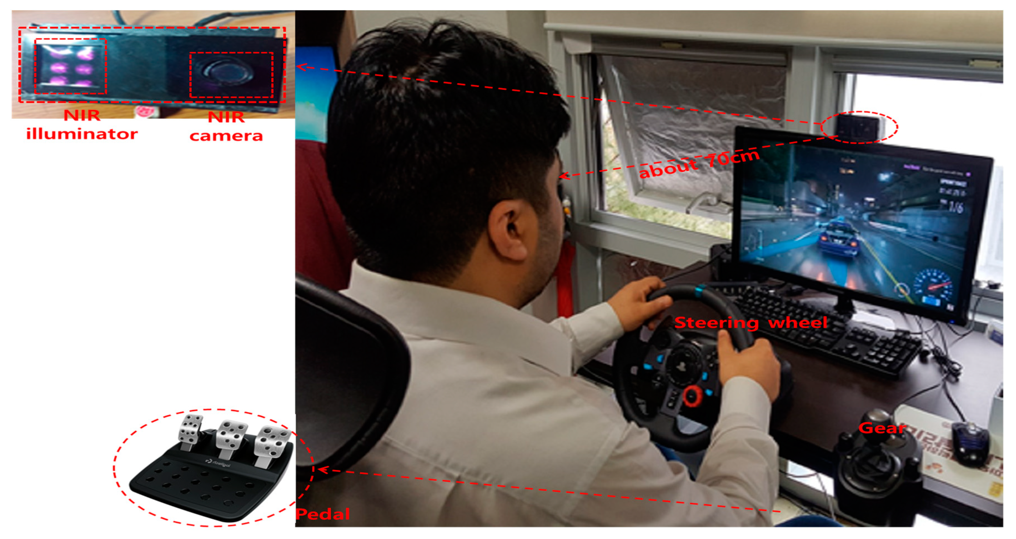
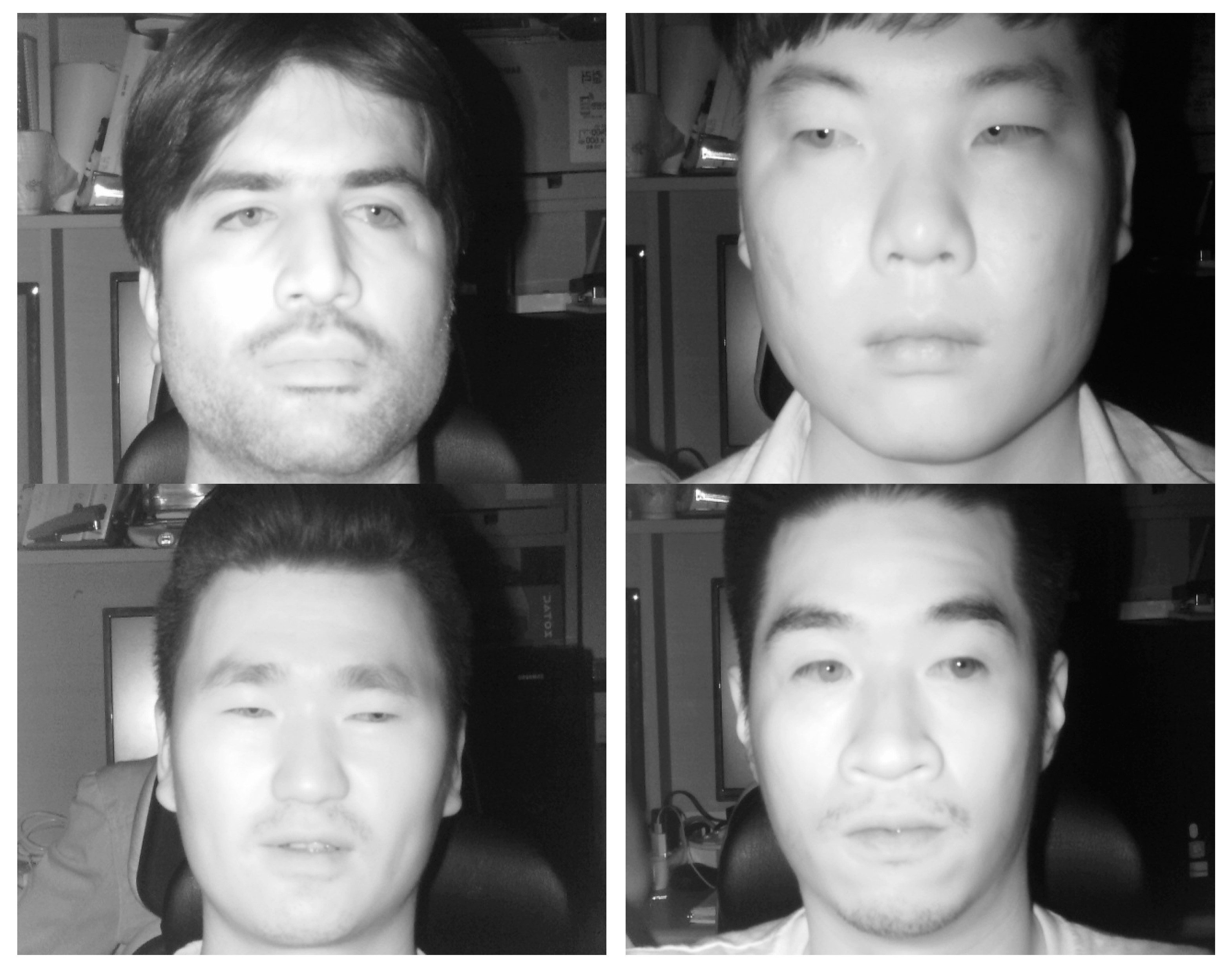
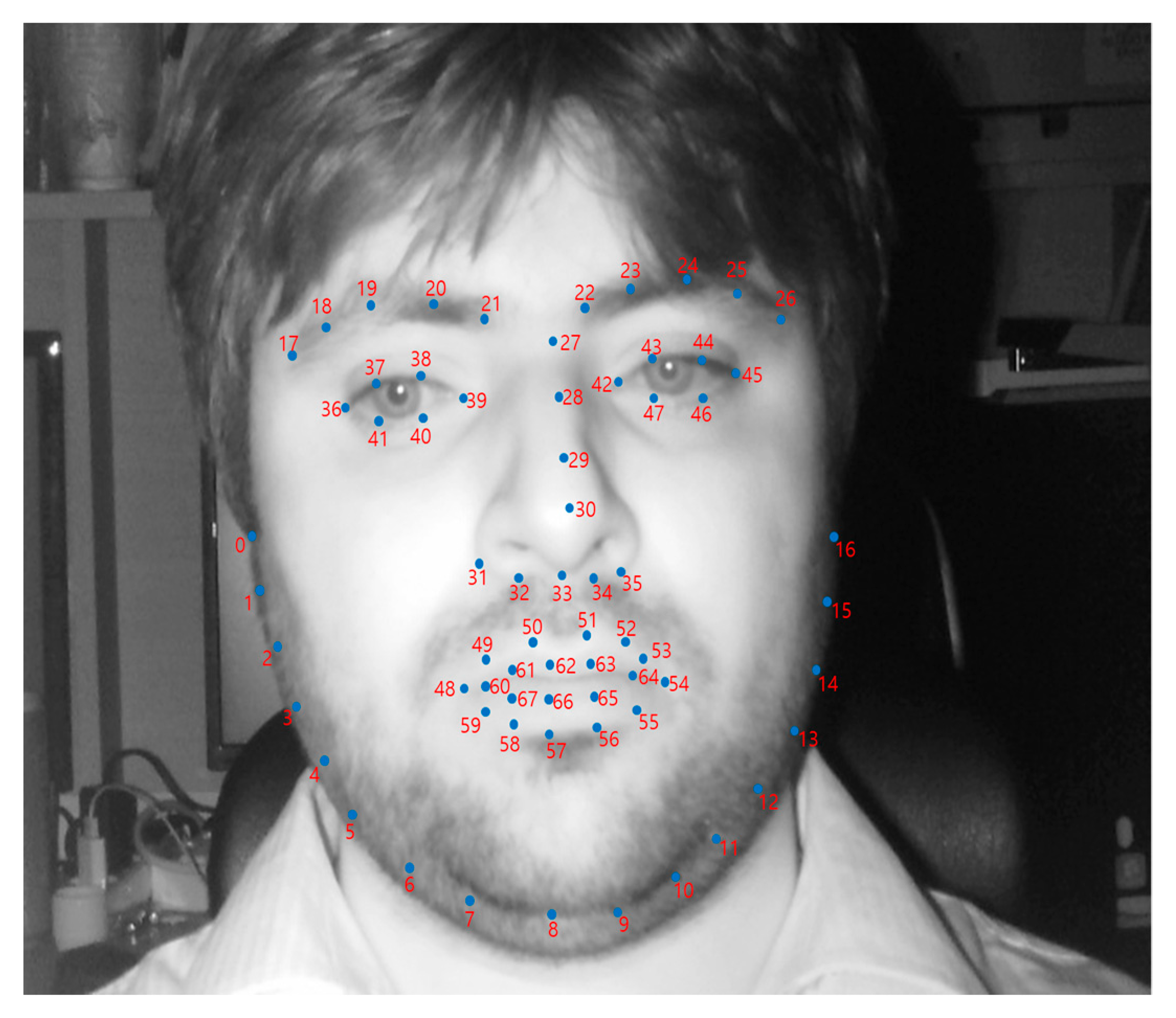
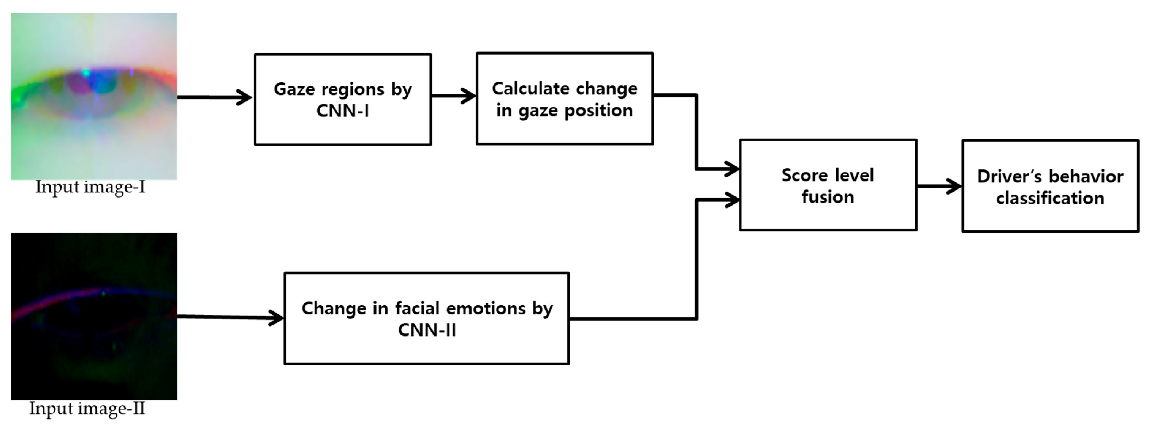
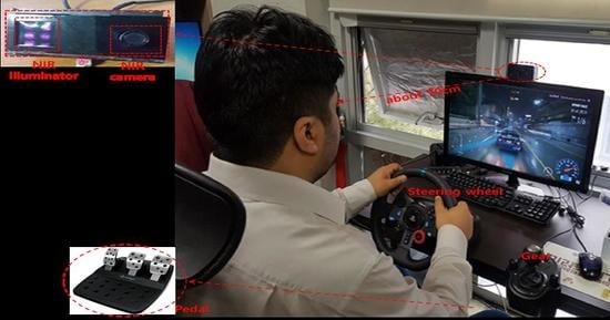
Figure 1 shows the flowchart of proposed method for driver’s facial emotion classification for aggressive and normal driving. As shown in steps (1), the NIR camera of our proposed system that is shown in Figure 2 captures the facial images of the user’s frontal view. A NIR camera and illuminator are installed on 24-inch monitor, which display a driving simulator. Aggressive and normal driving experiment is performed while using two types of driving simulators, as it can be dangerous in the real car environment. We have used steering wheel, gear shifter, and pedals for experiment of our all participants in order to give the feeling of real driving environment. Figure 2 shows the driving simulator and Section 4.1 discusses its details. Data acquisition is done while using NIR camera that was manufactured by ELP-USB500W02M [41]. To receive light in the NIR range, a 850 nm NIR band-pass filter is attached with the NIR illuminator [42]. NIR illuminator consists of six NIR light emitting diodes (LED), each LED’s wavelength is 850-nm [43]. The dimensions of obtained facial NIR images are of 640 × 512 pixels with eight bits each are used for data acquisition. Figure 3 shows the samples of the captured images of NIR camera. Obtained image is simultaneously feed into two Dlib facial feature trackers (the details are explained in Section 3.2). The region of interest (ROI) images are obtained based on the 68 facial landmarks that were obtained by Dlib facial feature trackers. The indices of the 68 coordinates of facial landmarks are shown in Figure 4. In Step (2), the ROI images of face, left, and right eye are obtained based on corresponding facial landmark by one Dlib. Similarly, in Step (4), the ROI images of mouth and left, and right eye are obtained based on a corresponding facial landmark while using second Dlib. Obtained ROI from the input NIR-image is used to extract three feature scores i.e., change in horizontal gaze (CHG) and change in vertical gaze (CVG) that are discussed in Section 3.2 and the change in facial emotions (CFE) is discussed in Section 3.3. These extracted feature scores are used to classify aggressive and normal driving based on the extracted feature scores. Classification will be done on the bases of score level fusion, which will be explained in Section 3.4.

3.2. Change in Horizontal and Vertical Gaze Positions

Gaze detection is used to locate the position where a user is looking at [44,45]. Eye gaze is considered to be an important cueing feature for analyzing driving behavior. It is quite obvious that eye movement while aggressive driving is very random and fast as compared to normal driving. Accordingly, change in gaze i.e., change in the horizontal and vertical gaze directions will be higher in case of aggressive driving as compared to the normal driving. Hence, in this research, we have exploited this cueing feature as an important factor to differentiate between the aggressive and normal driving behavior.
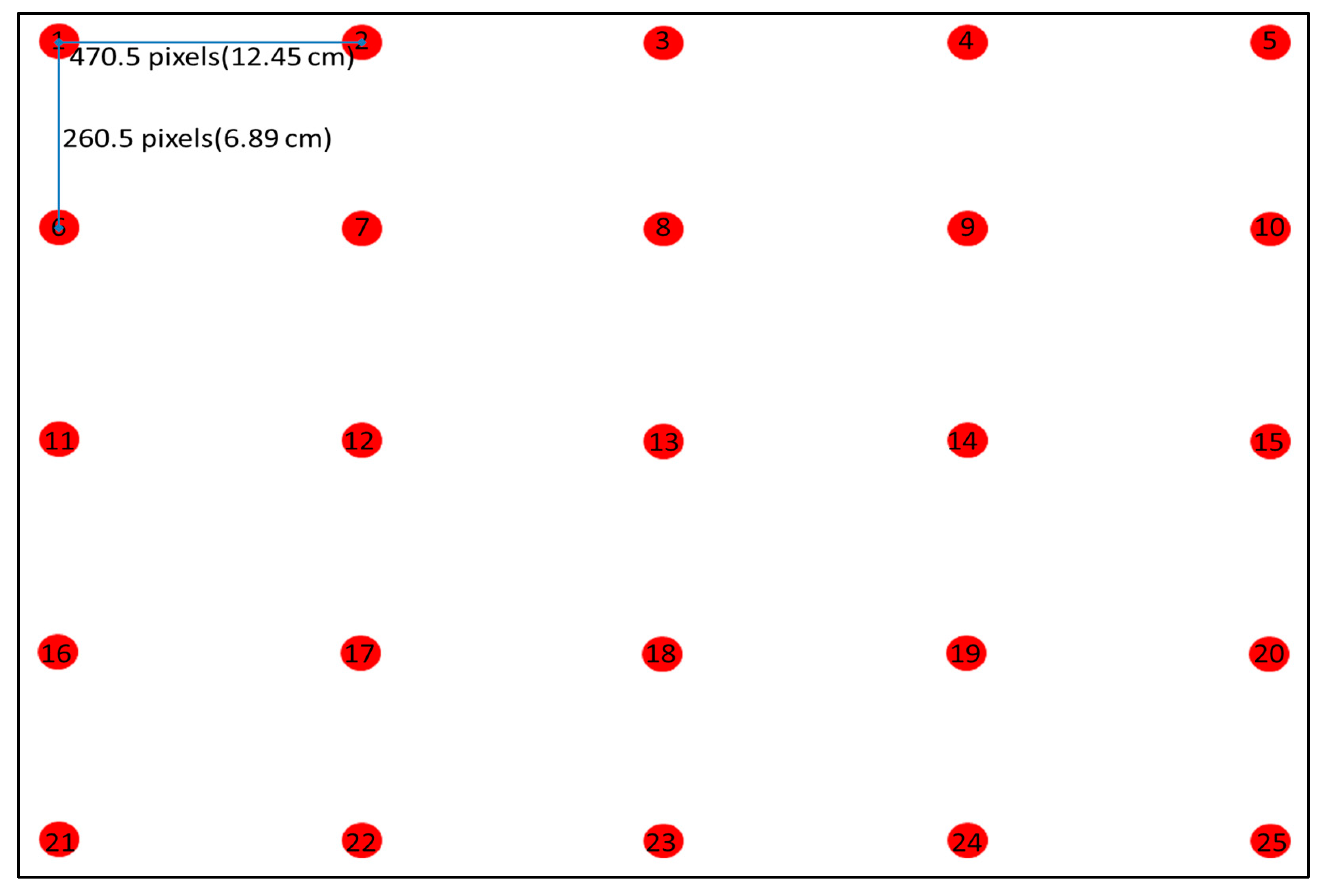
Gaze position is calculated based on the 25 gaze regions defined on the 24-inches monitor screen with resolution of 1920 × 1080 pixels, as shown in Figure 5. The size of circular target is 34 pixels for radius (9 mm for radius). The gaze regions are obtained by using the trained CNN-model (discussed in Section 3.4) for the desktop environment. Once the gaze regions are obtained, gaze position is calculated based on the obtained gaze regions. The current gaze position is horizontal and vertical position of gaze from the reference gaze region i.e., region 1, as shown in Figure 5. Hence, from the obtained gaze regions, change in gaze position is calculated by difference between the current and previous gaze position. That will be ultimately used to find change in horizontal and vertical gaze positions.
A change in horizontal and vertical gaze position is calculated by taking the average of absolute difference between current and previous frame gaze positions, as shown in Equations (1) and (2). Here, x and y are change in horizontal and vertical gaze positions, respectively. x i and y i are the current horizontal and vertical gaze positions, respectively. Similarly, x i 1 and y i 1 are the previous horizontal and vertical gaze positions, respectively, and n is the number of frames to be averaged for calculating the change in horizontal and vertical gaze positions i.e., five frames.
C h a n g e   i n   h o r i z o n t a l   g a z e   ( x ) =   1 n i = 1 n | x i x i 1 |
C h a n g e   i n   v e r t i c a l   g a z e   ( y ) = 1 n i = 1 n | y i y i 1 |
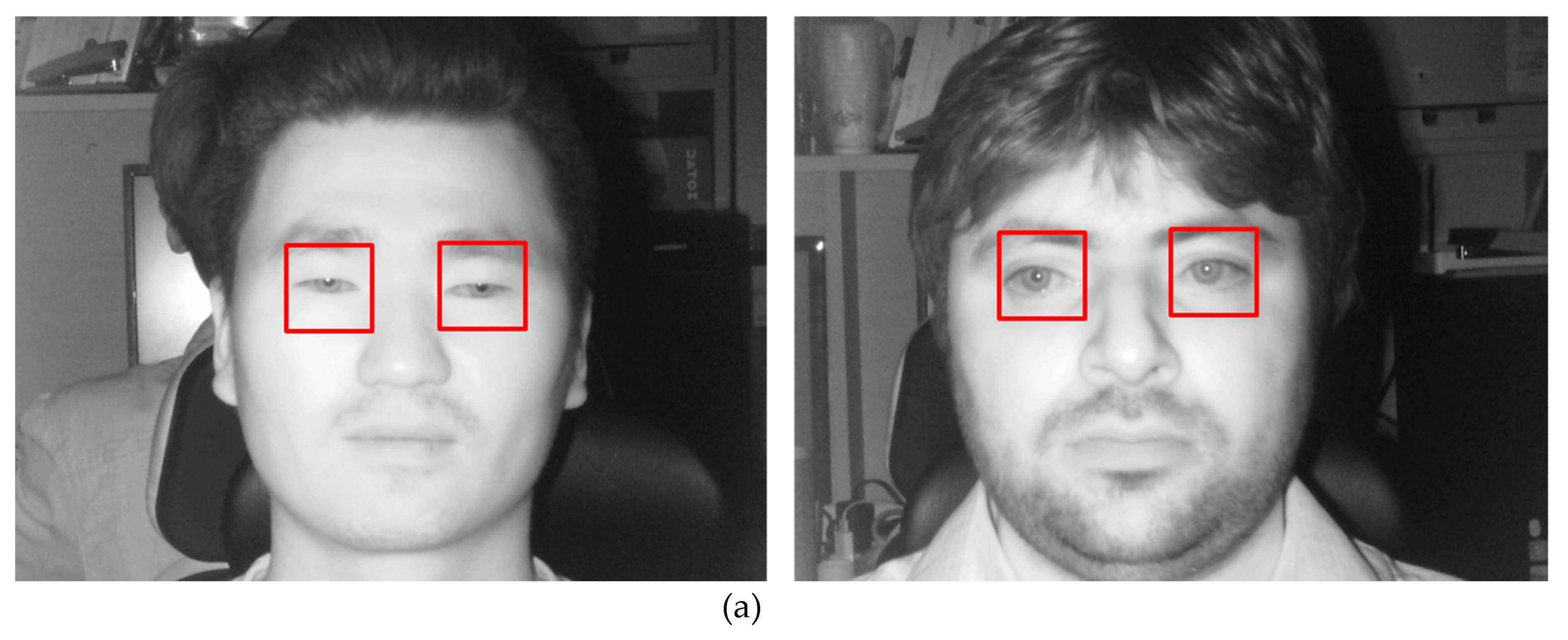
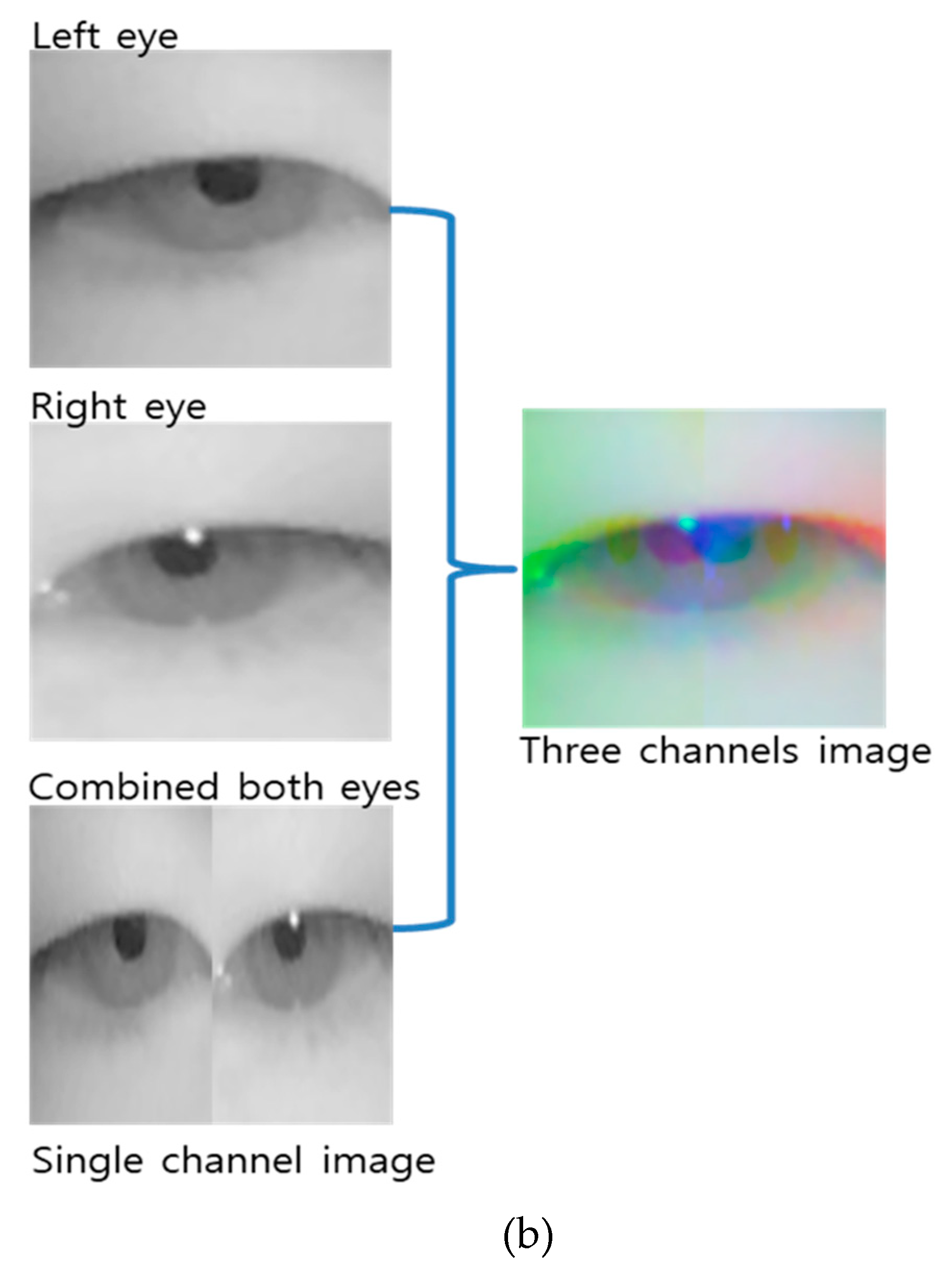
From the facial image, the change in gaze is calculated from defined ROIs of left eye, right eye, and combined left and right eye. Three channel images for calculating change in gaze are obtained by combining three single channel images of left eye, right eye, and combined left and right eye. Figure 6a shows the ROI on the original image and the three channel image that was obtained from the three single channel image is shown in Figure 6b.

3.3. Change in Facial Emotions

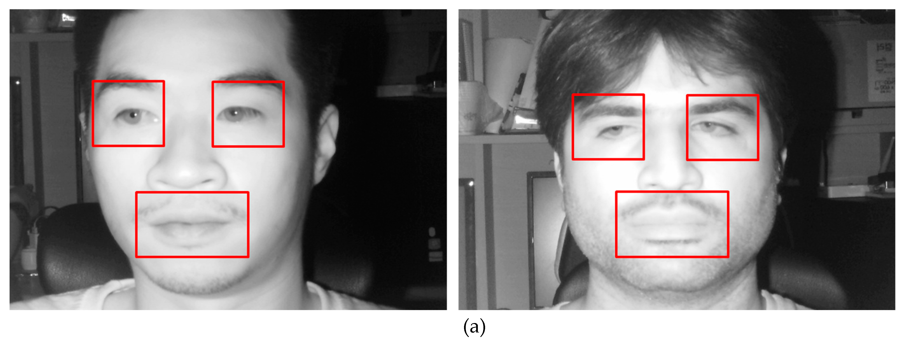
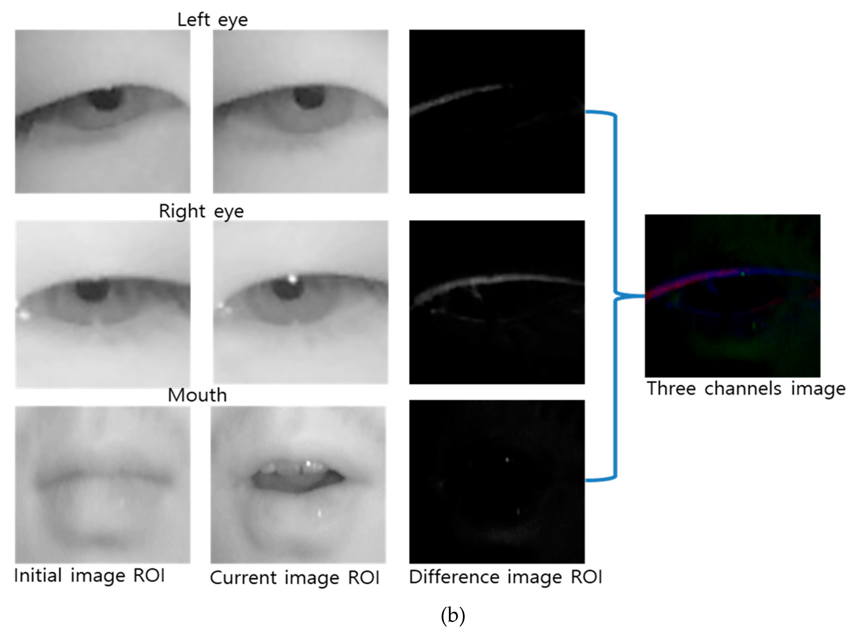
Ekman et al. studied emotional experience through facial signs [46]. In that they found that facial action provide accurate information about human emotions. The mouth and eyes are the main source of information on face area. Hence, in our system, we have extracted the facial emotions from the mouth and left and right eye ROI images, as shown in Figure 7a, with the center of feature points of the mouth and eyes that was previously defined, as shown in Figure 4. The difference images are obtained from the currently extracted three ROI images and previously stored three ROI images of both the eyes and mouth of driver. Previously stored three ROI images are the initial images of the driver when the vehicle starts show normal driving emotion. The variations that were obtained by the difference between the initial ROI images and current ROI images deduce aggressive driving. For facial emotions, the difference image and three channels image that were obtained from the three single channel images are shown in Figure 7b.

3.4. CNN Structure

Two images i.e., input image-I and input image-II, are obtained from Section 3.2 and Section 3.3, respectively. Input image-I is three channel image obtained in Section 3.2 i.e., change in gaze (Figure 6). Similarly, input image-II is three channel image obtained in Section 3.3 i.e., facial emotions (Figure 7). These two types of images are used as an input for CNN structures i.e., gaze regions by CNN-I and facial emotions by CNN-II, as shown in Figure 8. The output of gaze regions by CNN-I is 25 gaze regions that were obtained at the output layer of the CNN structure and output of facial emotions is facial feature scores obtained by CNN-II at the output layer of the CNN structure. Horizontal and vertical gaze change is calculated based on the gaze regions that were obtained at the output of CNN-I. Subsequently, the obtained change in gaze is combined with the facial feature score that was obtained from CNN-II through score level fusion. Hence, driver’s behavior i.e., aggressive or normal is classified on the basis of score level fusion.
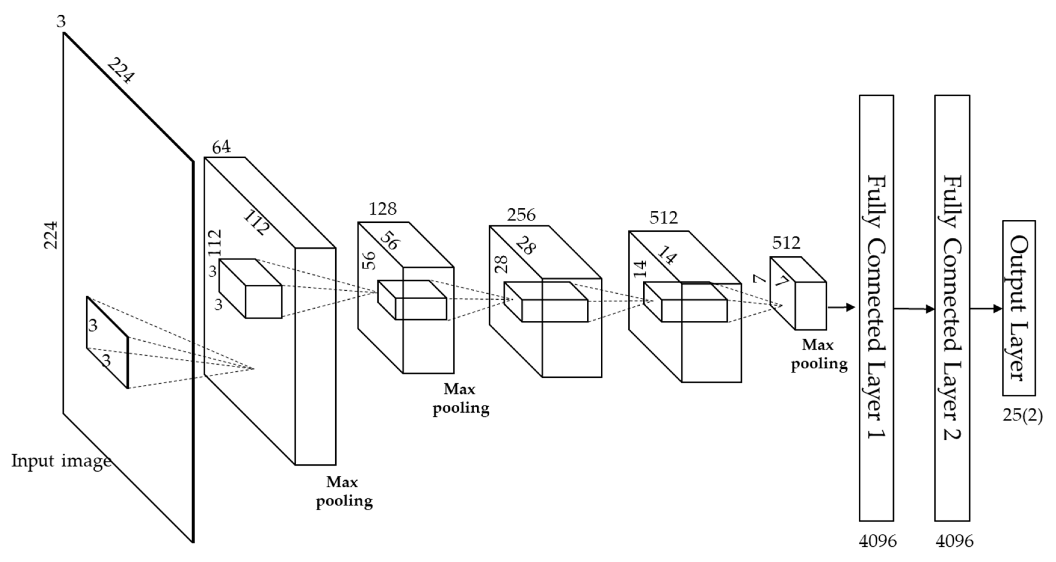
Table 2 and Figure 9 show the detailed CNN structure used in our proposed method. The VGG-face model is used in our proposed method [47]. It is comprised of 13 convolutional layers, five pooling layers, and three fully connected layers (FCLs). We have fine-tuned VGG-face with our self-collected database (DDBC-DB1). In the image input layer, an input image of size 224 × 224 × 3 is used. Here, 3 represents number of channels, while 224 × 224 is the width and height of the input image. Next comes the 1st convolutional layer (1st CL), which carries 64 filters of 3 × 3 size. The feature map of 224 × 224 × 64 is obtained from that. The following criteria are used for calculating this: (output height (or width) = (input height (or width)—filter height (or width) +2 × the padding number)/stride number +1) [48]. For example, in Table 2, the input height, filter height and the padding and stride number are 224, 3, 1, and 1, respectively. Therefore, the output height of the feature map by convolution is calculated as 224 (=224 − 3 + 2 × 1)/1 + 1). Usually, the output feature map for convolution that is based on padding and stride one is obtained by [49]:
Ok,l,n = Σi,j,m Ki,j,m,n · Ik+i−1,l+j−1,m
where Ok,l,n is the output feature map of the size of TF × TF × Q. Here, TF is the spatial height and width of a square output feature map and Q is the number of output channels (output depth). Ik+i−1,l+j−1,m is the input feature map of the size of SF × SF × P. SF is the height and width of square input feature map and P is the number of input channels (input depth). Additionally, Ki,j,m,n is the convolution kernel of size SK × SK × P × Q, and, here SK is the spatial dimension of convolution kernel. From that, standard convolutions have the following computational cost of:
C = SK · SK · P · Q · SF · SF
The above computational cost is multiplicatively based on the kernel size SK × SK, the number of input channels P, the number of output channels Q, and the input feature map size SF × SF [49].
The rectified linear unit (ReLU) layer is applied as a non-linear function. This function can prevent the vanishing gradient problem [50], which can be due to the hyperbolic, sigmoid, or tangent function used in back propagation for training. It has a faster calculation time than other activation functions. It is based on the following function [51,52].
y = max(0,x)
Here, x is the input value and y is the corresponding output value obtained from the ReLU function. By Equation (5), the result of y can be the max. of input x or 0. In addition, in case of input x is positive value, the y is same to x, and its derivative becomes 1, which makes the back propagation calculations easier. For these reasons, training efficiency increases because of the decreased total training time.
After going through the ReLU layer (ReLU-1_1), the feature map that was obtained from the second convolutional layer once again goes through the ReLU layer (ReLU-1_2) before it goes through the max pooling layer (Pool-1), as presented in Table 2. Here, the feature map size of the second convolutional layer is the same as in the first convolutional layer i.e., 224 × 224 × 64, with a filter of size 3 × 3, padding 1 × 1, and stride 1 × 1. The max pooling layer performs a kind of subsampling, in which the maximum value among the values defined in the filter range is selected. After passing through ReLU-1_2, the feature map size is 224 × 224 × 64. By using max pooling layer (Pool-1) that is shown in Table 2 with kernel size of 2 × 2, and stride of 2 × 2, the feature map size from 224 × 224 × 64 is reduced to 112 × 112 × 64, which is 1/4th of the original. There is no overlapping area because the max pooling filters of 2 × 2 moves two pixels in horizontal and vertical directions, as per the 2 × 2 stride.
It can easily be analyzed in Table 2 that, in all 13 convolutional layers, the size of kernel is 3 × 3, the padding size is 1 × 1, and the stride is of size 1 × 1. Only the entity changing is the number of filters i.e., 64, 128, 256, and 512. Before each ReLU layer, there is a convolutional layer. Similarly, the max pooling layer is used after each of the five groups (Group 1 to Group 5) of layers, as shown in Table 2. The size of filter in each max pooling layer is of 2 × 2, the stride of 2 × 2, and the padding of 0 × 0. As previously explained, at each max pooling layer, the feature map size is reduced, ReLU-1_2 (224 × 224 × 64) is reduced to Pool-1 (112 × 112 × 64), ReLU-2_2 (112 × 112 × 128) to Pool-2 (56 × 56 × 128), ReLU-3_3 (56 × 56 × 256) to Pool-3 (28 × 28 × 246), ReLU-4_3 (28 × 28 × 512) to Pool-4 (14 × 14 × 512), and ReLU-5_3 (14 × 14 × 512) to Pool-5 (7 × 7 × 512).
Once the CNN is trained on the training data after passing through above explained layers, the over-fitting problem is one more possible problem that can affect the outcome. This problem rises if CNN becomes too dependent on the training data. It can cause low classification accuracy with testing data, although the accuracy with training data is very high. We have come up with dropout methods that can reduce the effect of over-fitting to tackle this type of issue [47,53,54]. For dropout method, we used a dropout layer with probability of 50% to disconnect the previous layers at the first and second FCL.
In this study, we have designed the classification system for driver’s behavior based on two CNNs i.e., gaze regions by CNN-I and facial emotions by CNN-II. As the number of gaze regions for calculating change in gaze is 25, the output layer of gaze regions by CNN-I is 25 × 1, as shown in Table 2. Similarly, the number of classes for facial emotions is 2, so the output layer of facial emotions by CNN-II is also shown in Table 2 in brackets i.e., (2 × 1) to differentiate from the gaze regions by CNN-I i.e., 25 × 1.
In the third FCL i.e., Softmax layer, the probabilities to be utilized as the classification criterion are calculated. Each value that results from the softmax function indicates the probability of an input belonging to a certain class. The total sum of all probabilities will be equal to one. The following equation is utilized for this purpose [55].
σ ( z ) i = e z i n = 1 K e z n
Given that the array of output neurons is set to z, we obtain the probability of neurons belonging to the i t h class by dividing the value of the i t h element by the summation of the values of all the elements. The proposed method is considered to be standard for normalizing the probabilities between 0 and 1. The output value will be zero or some positive value by using input value of z into exponential function, which makes the training easier. Moreover, the range of output can be normalized by dividing numerator with summation of calculated value by exponential function, as shown in Equation (6). This prevents the training of weights that are affected by large output value. The final classification in the last layer chooses the classes with the highest probability among all of the values obtained by the Softmax regression [56] as the image classification result.

3.5. Score-level Fusion

Classification between aggressive and normal driving is done on the basis of score-level fusion of the features score obtained from two CNNs outputs i.e., gaze regions and facial emotions. The faze regions are further used to find horizontal and vertical change in gaze. Hence, horizontal and vertical change, combined with the facial emotions, are used to classify aggressive and normal driving. Horizontal and vertical change obtained from gaze regions of CNN-I are represented by feature score s1 and s2, respectively. Similarly, a facial emotion that is obtained from CNN-II is represented by s3. The final score is obtained by combining three feature scores and performance of weighted SUM and weighted PRODUCT rules are compared through Equations (7) and (8), which are shown below. The optimal weights for weighted sum and weighted product were selected by training data. Section 4.4 shows detailed explanations.
W S = i = 1 m w i s i
W P = i = 1 m s i w i
Here, m is 3, as we are dealing with three feature scores i.e., i of 1, 2, and 3 show the horizontal change, vertical change, and facial emotion, respectively. WS and WP are the scores by weighted SUM and weighted PRODUCT rules, s i is the score that is obtained from the features, and w i is the weights. The optimal rule is determined to have the least error in classifying aggressive and normal driving emotions via training data.

4. Experimental Results

4.1. Experimental Data and Environment

In this research, we have collected our own database (DDBC-DB1) for the classification of aggressive and normal driving behavior, as shown in Figure 3. The database is collected through the experimental setup, which can be viewed in Figure 2. As mentioned before, it is dangerous to collect data in a real car environment, so very few works has been done until now due to the complexity of the task. If any database is collected that is not open access for academic use, as they may be prepared by auto industry or security agencies for their personal use. Therefore, we have collected our own database (DDBC-DB1) for aggressive and normal driving behavior. The database was collected from 20 participants of different nationalities between ages of 23 to 34 years, in the experiment. Out of 20 participants, 12 were male and eight were female, in which four were wearing glasses. All of the participants voluntarily participated in the experiments. A presentation demo was given to the participants before the experiment, in which all of the details and purpose was presented. Once they completely understood the purpose and procedure of experiments, written consent was taken from all of the participants. We have utilized two types of driving simulators to create aggressive and normal driving situation in our lab. For aggressive driving, the competition mode of Need for Speed (Deluxe Edition) [57] was used and normal driving, and the autonomous mode of Euro Truck Simulator 2 [58] was selected, as they were considered to be most appropriate for this situation.
Our experiment consists of two parts: In first part of our experiment, we trained our CNN model for calculating the change in gaze. For this purpose, 25 gaze spots (gaze regions) were designated, as shown in Figure 5, and each of the 20 participants stared at designated spots in the mentioned numeric sequence turn by turn and at each spot 30 image frames were extracted. Each participant repeated the same experiment five times. Hence, we have collected 3000 images for each gaze spot from this experimental environment. Accordingly, for 25 gaze spots, 75,000 images were collected that are used for training and testing CNN structure, as shown in Figure 9. We divided the collected data into two equal parts to perform two-fold cross validation for training and testing data. The average accuracy of gaze detection that was achieved by our trained CNN model for desktop environment is 69.7% (“need to calculate in degrees while using weighted sum of obtained scores”). The CNN based gaze detection system in actual car environment proposed in our previous research [59] has shown an accuracy of 92.8%, which is much higher than the desktop environment. Gaze detection accuracy is very low for desktop environment while using CNN model because of the very less distance between designated the gaze spots, as shown in Figure 5. However, in the actual car environment, the distance between the gaze regions is enough for differentiating between gaze regions. Hence, it is probable that, once we deploy our proposed prototype in actual car environment, a change in gaze feature will be more effective when compared to the desktop environment.
In second part of experiment, we need to train our CNN model for obtaining feature scores for change in facial emotions. We used same 20 participants for collecting data for aggressive and normal driving. In this experiment, facial emotions were recorded while using the experimental setup that is shown in Figure 2. It includes five minutes of normal driving while using a Euro truck driving simulator and another five minutes of aggressive driving was recorded while using need for speed driving simulator, similar to the one used in [29] i.e., multi-camera based system. Each participant watched a sequence of neutral images for five minutes from the international affective picture system to maintain neutral emotion input [60]. We have used 24-inch monitor from Samsung company with model number: LS24D300HLS [61]. Figure 10 illustrates the steps followed during the experimental procedure. Three trials are performed for this experiment for each participant with gap of 10 min for rest.
In our experiment, we performed two-fold cross validation for training and testing. For that purpose, we have randomly divided our database into two equal subsets, as shown in Table 3. During the first fold, a subset of ten people was used for training and remaining ten were used for testing. Similarly, during second fold, training and testing data are interchanged i.e., second subset of ten participants for testing and first subset was used for training and validation is performed based on the testing data.
Windows Caffe (version 1) [62] was used for the implementation of training and testing algorithm of the CNN model. For the training and testing of CNN, we used a desktop computer with an Intel® Core™(Santa Clara, CA, USA) i7-3770K CPU @ 3.50 GHz, 16 GB memory, and a NVIDIA GeForce GTX 1070 (1920 CUDA cores and 8 GB memory) graphics card [63]. Our algorithm was implemented by Microsoft Visual Studio 2013 C++, and OpenCV (version 2.4.5) [64] library and Boost (version 1.55.0) library.

4.2. Extracted Features and the Comparison of Performance

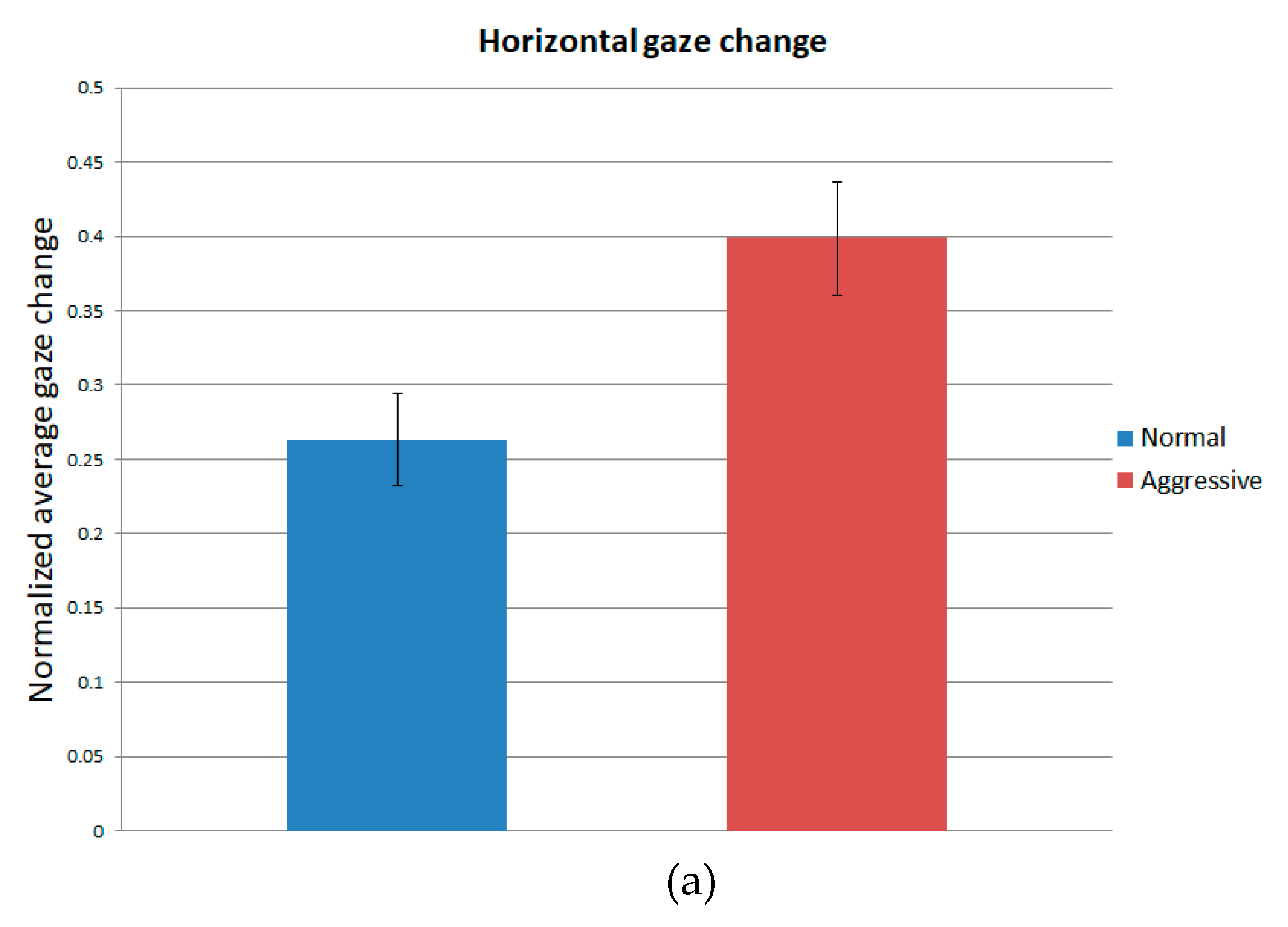
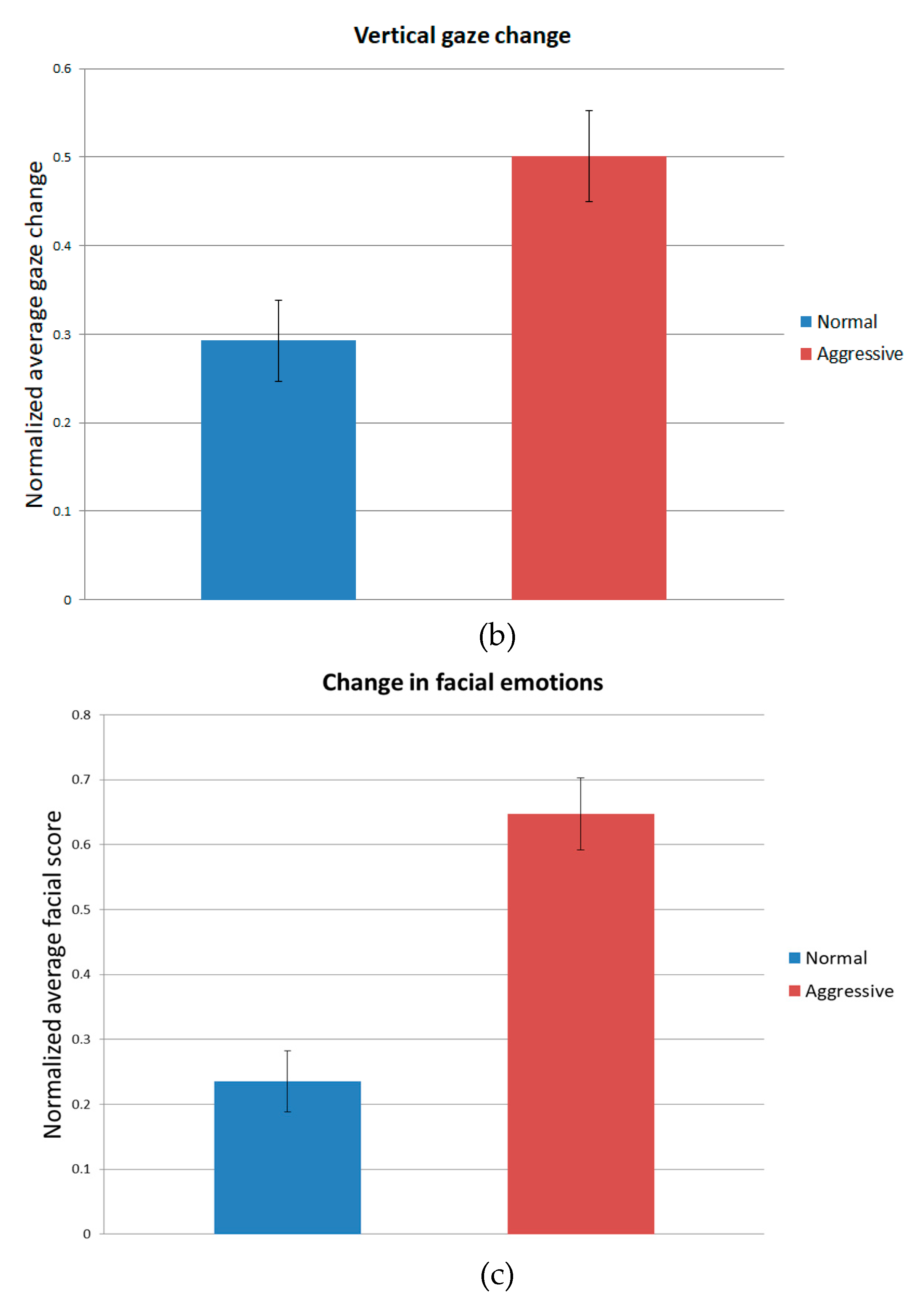
As mentioned in Section 3.1, we are using three features i.e., change in horizontal gaze, change in vertical gaze and change in facial emotions for classification of aggressive and normal driving. Here, we will compare which feature is more effective from the other one. Change in gaze was extracted from RGB (three channels) image obtained from three ROIs of a NIR image, as was explained in Section 3.2 (see Figure 6). Once CNN is trained with the training data, features scores for gaze region can be extracted from the output of the first CNN. On the basis of gaze regions that were obtained from the feature score, a change in horizontal and vertical gaze positions was calculated. Similarly, the third feature for facial emotions of driver is extracted based on the feature scores obtained at the output of the second CNN. We compared three feature score values to analyze effectiveness and strength of each feature for classifying aggressive and normal driving emotions. We have summarized the comparison results for the feature vales in Table 4 and Figure 11. The average and standard deviation is calculated for each feature during aggressive and normal driving. It can be noted that average value for aggressive driving is higher for all three features when compared to the normal driving.
We have also conducted the t-test [65] and Cohen’s d analysis [66] for feature values collected while aggressive or normal driving. In the null hypothesis for t-test, it is assumed that there is no difference between the features during aggressive and normal driving. The null hypothesis is rejected at a 99% confidence level, as the p-value for all three features is less than 0.01, indicating that there is a difference of 99% confidence level between aggressive and normal driving features. Similarly, if the p-value that is obtained by t-test is 0.05 or less than that, null hypothesis is rejected by the 95% confidence level. It means the difference of features between aggressive and normal driving is 95%. Hence, it can be analyzed through the obtained result that, if the p-value decreases, then there is significant level of difference between measured datasets. The Cohen’s d method is used for analyzing the reliability of the observed phenomena. It gives the difference of image features between two average values and then divided by standard deviation. Strength or effect sizes such as small, medium, and large are defined by Cohen’s d values of 0.2, 0.5, and 0.8, respectively. Medium and large strength indicates higher reliability when compared to the small strength values in terms of difference between the observed values.
It is clearly differentiated in Table 4 and Figure 11 that the three feature value used in this research in the form of mean, standard deviation, p-value, Cohen’s d value, and strength. In Figure 11, “Normal” and “Aggressive” indicates normal driving and aggressive driving, respectively. It can be observed that the p-value for a facial feature is less than change in horizontal and vertical gaze. Hence, the change in facial emotions feature is more reliable than the change in horizontal and vertical gaze features for classifying aggressive and normal driving. Additionally, Cohen’s d value for the change in facial emotions feature is higher than other two features i.e., change in horizontal and vertical gaze. Consequently, the facial features are more effective than the classification of aggressive and normal driving.

4.3. Training of CNN Model

The training of the CNN model or teaching of the CNN model is more or less used in the same context. The stochastic gradient descent (SGD) method i.e., one of the back-propagation methods was used to teach our CNN [67]. Back propagation is an approach that is used to learn the weight of connections in neural networks. The SGD algorithm optimizes the parameters by computing derivatives of the difference between the expected and obtained out values. The well known parameters that are used for the SGD method are mini-batch size, learning rate, learning rate drop factor, learning rate drop period, L2 regularization, and momentum. The definition of the parameters elaborated in [68]. The parameters that are used in our SGD algorithm are represented in the tabular form that is shown in Table 5. In SGD method, division of the training set is defined via mini-batch size iterations and states the operation of training duration as 1 epoch. During the training process, an input is pre-labeled with the correct original class. If the input labeled sample goes through the neural network with forward direction, the expected and obtained outputs acquired from the neural network can be either the same or different. In case of difference between the desired and actual outputs, the learning rate is multiplied and results are applied when new weight values are updated. The filter coefficients and weights are learned by convolutional layers and fully connected layers of the CNN, respectively, while using the SGD method.
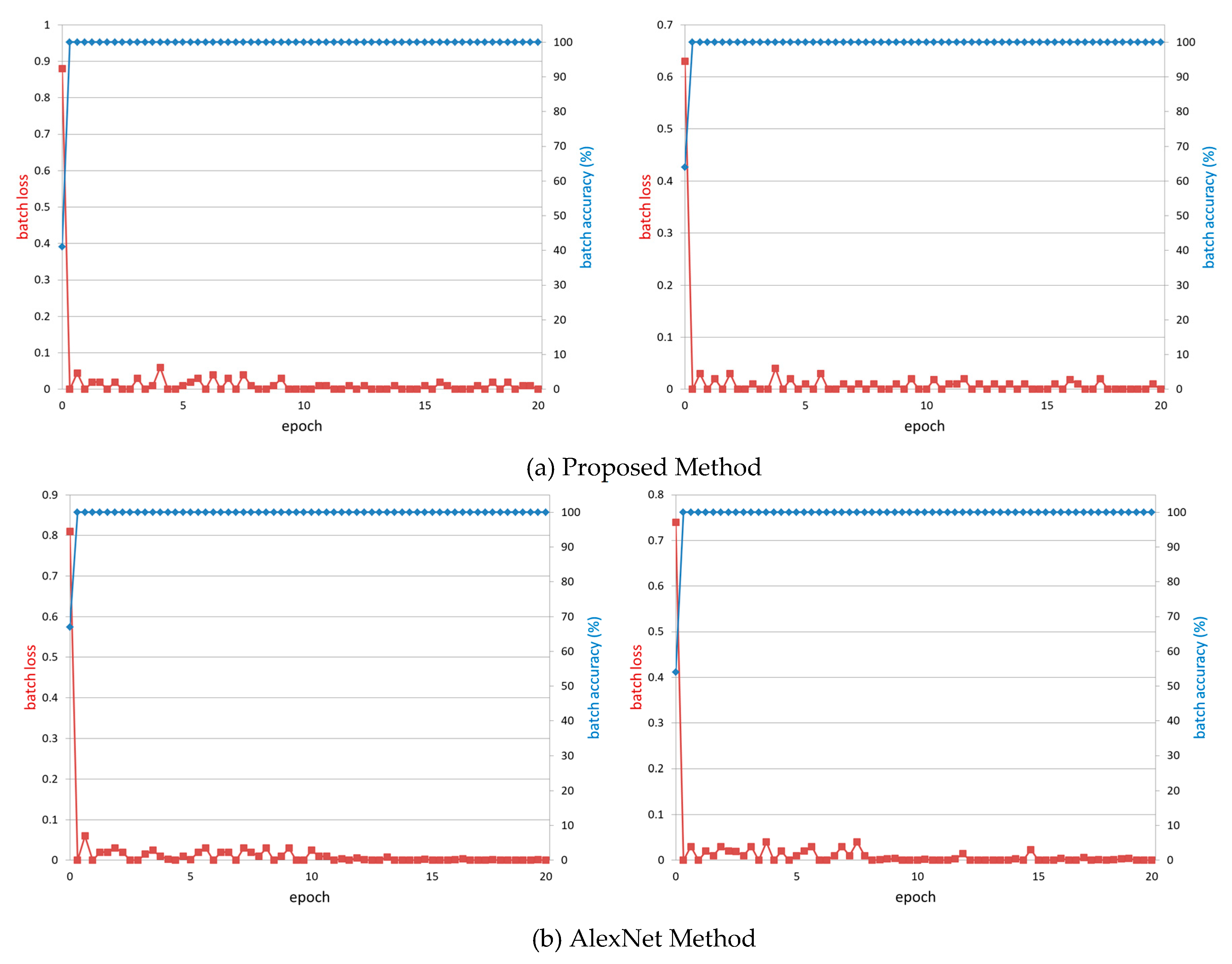
Figure 12 shows the graphs of accuracy and loss for each epoch during the training step for the two-folds of cross validations for the proposed and AlexNet method i.e., Figure 12a,b, respectively. In all cases, the training loss values are close to 0 while the accuracy approaches 100% as the training epoch increases. This proves that the training of the proposed method is sufficient with the training data. When compared to the typical training of CNN structure, the fine-tuning manner is based on the trained CNN model, and the convergence speed of accuracy and loss by fine tuning method is faster than that by typical training.

4.4. Testing of CNN Model

In our research, we have measured the accuracy of the aggressive and normal driving behavior classification by calculating the equal error rate (EER) between aggressive and normal driving. For differentiating purpose, we have considered that the data obtained through aggressive driving are true positive (TP) and normal driving data are considered as true negative (TN). The TP data are collected when each of the 20 participants were playing Need for Speed (Deluxe Edition) while using our driving simulator. The TN data were collected when each participant played Euro Truck Simulator 2 using our driving simulator. On the basis of these definitions, two more cases can be defined i.e., false negative (FN) and false positive (FP). False negative is the case when aggressive driving is misclassified as normal driving; whereas, FP is the case in which normal driving is incorrectly recognized as aggressive driving. On the basis of this, we can define false positive rate (FPR) and false negative rate (FNR). Similarly, two accuracies defined before can be assumed as true positive rate (TPR) and true negative rate (TNR). TPR is calculated as 100 − FNR (%), and TNR is calculated as 100 − FPR (%).
Firstly, we have analyzed classification accuracy from each of the proposed input features i.e., change in horizontal gaze position (CHG), change in vertical gaze position (CVG), and change in facial emotions (CFE) value separately. In Table 6, we have shown confusion matrices of the results obtained for first fold, second fold, and their average through VGG-face 16 model.
As explained in Section 3.5, the scores of the inputs i.e., change in gaze and facial emotions are combined by weighted SUM or weighted PRODUCT rules shown in Table 7 and Table 8, respectively. Through training data, the optimal weights for these rules were determined. The optimal weights for horizontal change in gaze, vertical change in gaze, and change in facial emotions using weighted SUM rule are 0.19, 0.21, and 0.60, respectively, with EER of 1.1%. Similarly, the optimal weights for horizontal change in gaze, vertical change in gaze, and change in facial emotions using weighted PRODUCT rule are 0.19, 0.21, and 0.60, respectively, with EER of 2.6%. It can be easily analyzed that EER obtained through weighted SUM is less than the weighted PRODUCT. A higher weight was determined for facial emotions as compared to the change in horizontal and vertical gaze, because facial emotions are calculated through the combined effect of mouth and eyes as compared to change in gaze obtained only through eyes. As shown in Table 4 and Figure 11, the horizontal and vertical change in gaze have almost similar strength, hence the determined weights have a very minor difference of 0.02. This is possibly due to the fact that vertical change is more sensitive when compared to the horizontal change in gaze, as shown in Figure 5. Consequently, a larger weight was determined for vertical change than horizontal change. In addition, we used weighted SUM in this study, because weighted SUM rule outperformed the weighted PRODUCT rule.
In Table 9, we have shown the confusion matrices of the results obtained for first fold, second fold, and their average through score-level fusion of input feature values. It can be seen that our method have shown the classification accuracy for first and second fold is 99.03 and 98.83, respectively. Hence, we achieved the average accuracy of 98.93% with our proposed method.

4.4.1. Comparison with Previous Methods

The first experiment compared the results that were obtained by CNN used in our proposed method i.e., VGG face-16 with previous methods [53] i.e., AlexNet method with fewer layers. We have used same data for training and testing AlexNet with two folds cross validation.
We have analyzed classification accuracy for each of the input features, the same as for our proposed method, i.e., change in horizontal gaze position, change in vertical gaze position, and change in facial emotions through AlexNet method separately. In Table 10, we have shown confusion matrices of the results obtained for first fold, second fold, and their average through the AlexNet model [53].
In Table 11, we have shown confusion matrices of the results obtained for first fold, second fold, and their average through score-level fusion of input feature values in terms of TPR, TNR, FNR, and FPR through the AlexNet model [53].
Table 9 and Table 11 show the confusion matrices of the proposed (VGG-face 16) model and previous AlexNet model in terms of TPR, TNR, FNR, and FPR. It can be easily analyzed from Table 9 and Table 11, which proposed VGG face-16 model that outperformed the previous AlexNet model in classifying aggressive and normal driving.
We have also compared the classification accuracy by using the HOG with a modified Hausdorff distance method (MHDM) [37]. The Hausdorff metric is used to measure how two test subsets i.e., aggressive and normal driving images are separate from each other. It is found that the average accuracy of two folds cross validation achieved through modified Hausdorff distance is 74.58%. It is also less than previous AlexNet method [53], as well as far less than our proposed method.

4.4.2. Comparison with Open Database

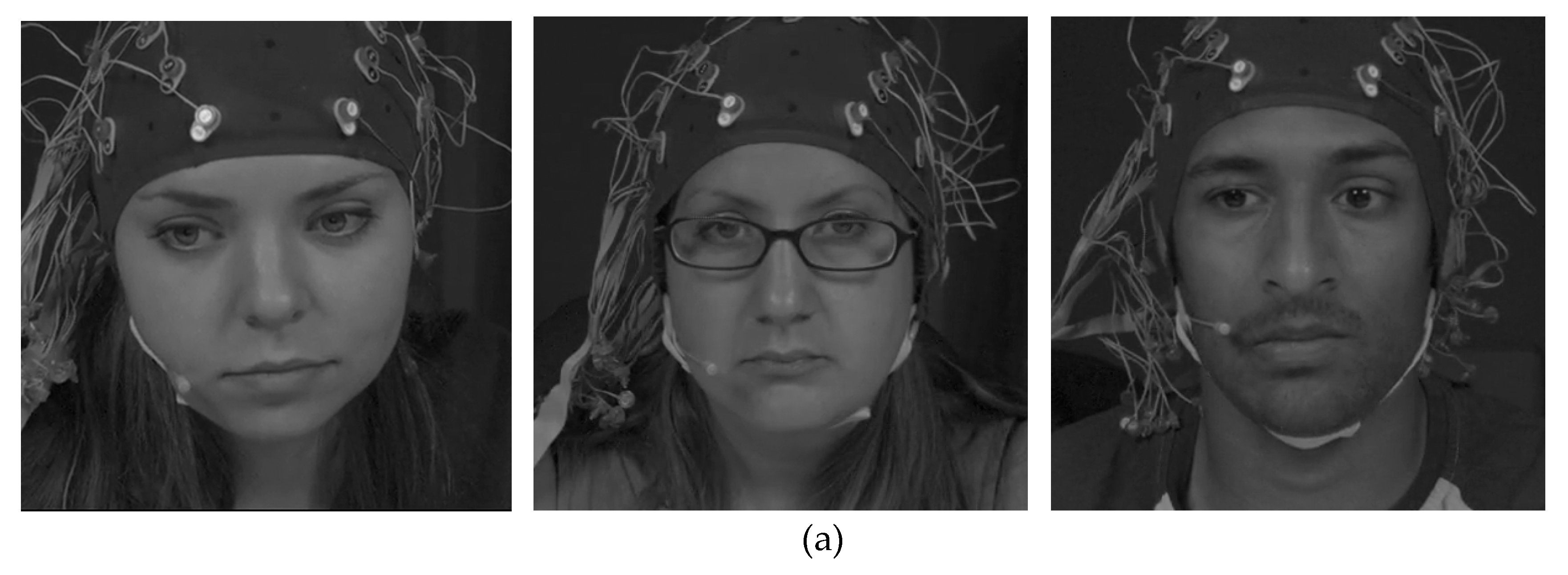
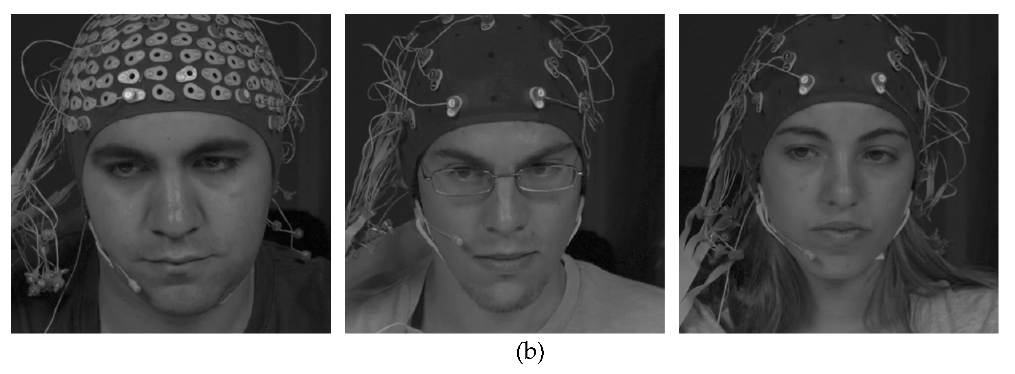
In the next experiment, we compared the accuracies by our proposed method with those by the previous method on MAHNOB HCI tagging database collected by Professor Pantic and the iBUG group at Imperial college London, and, in part, collected in collaboration with Prof. Pun and his team of University of Geneva, in the scope of MAHNOB project financially supported by the European Research Council under the European Community’s 7th Framework Programme (FP7/2007-2013)/ERC Starting Grant agreement No. 203143 [69]. It is a large facial expression database with 30 participants with different cultural and education backgrounds. They collected audio, video, gaze, and physiological data in response to emotion-eliciting video clips. They performed emotion elicitation experiment, which include response to different emotional videos as stimuli. They selected 12 different emotions, such as sadness, joy, anger, fear, surprise, neutral, etc. We have chosen two emotions, such as anger for aggressive driving emotion and neutral for normal driving emotion, most suitable to our requirement. In the MAHNOB HCI tagging database [69], they have used six video cameras for recording facial expression and head pose from different angles. We have extracted our required information for change in facial emotions and gaze position from image frames that were obtained from video obtained from frontal view camera. Figure 13 shows the examples of facial images with aggressive and normal emotion.
In Table 12 and Table 13, we have shown the confusion matrices in terms of TPR, TNR, FNR, and FPR that were obtained through the proposed and previous [53] method on open database [69], respectively.
Similarly, we have verified the modified Hausdorff distance method [37] on an open database. It has shown the accuracy of 64.51%. Note that with open database, our proposed method have shown accuracies of 91.36% and 89.92% for first fold and second fold validation with an average of 90.64%, which is much higher than the average accuracy by the previous method [53] and modified Hausdorff distance method [37] i.e., 75.85% and 64.51%, respectively.

4.4.3. Comparison with Receiver Pperation Characteristic (ROC) Curves

Figure 14 show the receiver operating characteristic (ROC) curves for the classification results of aggressive and normal, according to different methods. The horizontal and vertical axes indicate FRP and TPR, respectively. It compares the classification accuracy of the proposed method with the previous method [53] and modified Hausdorff distance method [37] on our own database (DDBC-DB1), as shown in Figure 14. The ROC curves show the average of the results that were obtained from two folds cross validation. It can be analyzed from the obtained ROC curves that our proposed method with score level fusion had the highest accuracy when compared to the previous method (ALexNet) [53] and the modified Hausdorff distance method (MHDM) [37] on our own database (DDBC-DB1).
Later, we verified the results of ROC curves on open MAHNOB HCI tagging database [69], as shown in Figure 15. It can be analyzed in the form of ROC curves that our proposed method has also been shown to be better when compared to the previous method (AlexNet) [53] and the modified Hausdorff distance method (MHDM) [37] on open database [69].
For classification problems, there is another important metrics to compare the results that were obtained by different methods [70]. Accuracy can be measured by following the four criterions shown in Equations (9) to (12), which are based on TP, TN, FP, and FN.
Positive   predictive   value   ( PPV ) = # TP # TP + # FP
TPR = # TP # TP + # FN
Accuracy   ( ACC ) = # TP + # TN # TP + # TN + # FP + # FN
F score = 2 · PPV · TPR PPV + TPR   ,
Table 14 shows the calculations of accuracy based on above defined criteria. In Equations (9) to (12), #TP, #TN, #FP, and #FN are the numbers of true positive, true negative, false positive, and false negative, respectively. The lowest and highest accuracy values of PPV, TPR, ACC, and F_score were 0% and 100%, respectively. It can noticed that our proposed method has outperformed other methods in all defined criterions and metrics. As a whole, the proposed method in this research has shown the best results when compared to other methods, as shown in Table 14.

5. Conclusions

In this study, we have proposed a method of driver’s behavior i.e., aggressive or normal driving classification while using a driving simulator based on CNN. For driving behavior classification, the proposed CNN model uses a driver’s change in horizontal and vertical gaze and also change in facial emotions obtained using single NIR light camera. For this purpose, change in gaze is calculated by left and right eye, change in facial emotions are collected by left eye, right eye, and mouth from an input image based on the ROI while using Dlib facial feature tracker. We have undertaken fine tuning with a pre-trained CNN model separately for the required feature values of gaze and facial emotions change. Separate scores for gaze and facial emotions change are extracted from fully connected layer of the VGG-face network. Three features i.e., horizontal change in gaze, vertical change in gaze, and change in facial emotions, are combined through score level fusion to find the final result of aggressive and normal driving classification. We compared the performance of the proposed method of driver’s driving behavior with previous methods. Evaluations were also performed on the open MAHNOB HCI tagging database. It is verified from the results that the driver’s behavior classification with our proposed method outperformed the previous methods. It can be analyzed through confusion matrix as well as ROC curves.

Author Contributions

R.A.N., W.-K.L. and A.P. designed the system for classification of aggressive and normal driving based on CNN. In addition, they wrote and revised the paper. M.A., A.R. and A.U.R. helped to implement the proposed system, comparative experiments, and collecting databases. W.-K.L. and A.P. provided the review and suggestions for the contents improvements. All authors have read and agreed to the published version of the manuscript.

Funding

This research was supported by the National Research Foundation of Korea (NRF) grant funded by the Korean government (MSIT) (No. 2018R1A2B6009188).

Acknowledgments

This research was supported by Basic Science Research Program through the National Research Foundation of Korea (NRF) funded by the Ministry of Education (NRF-2015R1D1A1A01056761), and in part by the Bio & Medical Technology Development Program of the NRF funded by the Korean government, MSIP (NRF- 2016M3A9E1915855).

Conflicts of Interest

The authors declare no conflict of interest.

References

  1. Global Status Report on Road Safety. 2015. Available online: http://apps.who.int/iris/bitstream/10665/189242/1/9789241565066_eng.pdf?ua=1 (accessed on 26 February 2018).
  2. Aggressive Driving: Research Update. Available online: http://www.adtsea.org/Resources%20PDF’s/AAA%202009%20Aggressive%20Driving%20Research%20Update.pdf (accessed on 26 February 2018).
  3. Chen, Z.; Yu, J.; Zhu, Y.; Chen, Y.; Li, M. D3: Abnormal Driving Behaviors Detection and Identification Using Smartphone Sensors. In Proceedings of the 12th Annual IEEE International Conference on Sensing, Communication, and Networking, Seattle, WA, USA, 22–25 June 2015; pp. 524–532. [Google Scholar]
  4. Bhoyar, V.; Lata, P.; Katkar, J.; Patil, A.; Javale, D. Symbian Based Rash Driving Detection System. Int. J. Emerg. Trends Technol. Comput. Sci. 2013, 2, 124–126. [Google Scholar]
  5. Coughlin, J.F.; Reimer, B.; Mehler, B. Monitoring, Managing, and Motivating Driver Safety and Well-Being. IEEE Pervasive Comput. 2011, 10, 14–21. [Google Scholar] [CrossRef]
  6. Lin, C.-T.; Liang, S.-F.; Chao, W.-H.; Ko, L.-W.; Chao, C.-F.; Chen, Y.-C.; Huang, T.-Y. Driving Style Classification by Analyzing EEG Responses to Unexpected Obstacle Dodging Tasks. In Proceedings of the IEEE International Conference on Systems, Man, and Cybernetics, Taipei, Taiwan, 8–11 October 2006; pp. 4916–4919. [Google Scholar]
  7. Zheng, W.-L.; Dong, B.-N.; Lu, B.-L. Multimodal Emotion Recognition Using EEG and Eye Tracking Data. In Proceedings of the 36th Annual International Conference of the IEEE Engineering in Medicine and Biology Society, Chicago, IL, USA, 26–30 August 2014; pp. 5040–5043. [Google Scholar]
  8. Koelstra, S.; Muhl, C.; Soleymani, M.; Lee, J.-S.; Yazdani, A.; Ebrahimi, T.; Pun, T.; Nijholt, A.; Patras, I. DEAP: A Database for Emotion Analysis Using Physiological Signals. IEEE Trans. Affect. Comput. 2012, 3, 18–31. [Google Scholar] [CrossRef] [Green Version]
  9. Khushaba, R.N.; Kodagoda, S.; Lal, S.; Dissanayake, G. Driver Drowsiness Classification Using Fuzzy Wavelet-Packet-Based Feature-Extraction Algorithm. IEEE Trans. Biomed. Eng. 2011, 58, 121–131. [Google Scholar] [CrossRef] [PubMed] [Green Version]
  10. Kamaruddin, N.; Wahab, A. Driver Behavior Analysis through Speech Emotion Understanding. In Proceedings of the IEEE Intelligent Vehicles Symposium, San Diego, CA, USA, 21–24 June 2010; pp. 238–243. [Google Scholar]
  11. Nass, C.; Jonsson, I.-M.; Harris, H.; Reaves, B.; Endo, J.; Brave, S.; Takayama, L. Improving Automotive Safety by Pairing Driver Emotion and Car Voice Emotion. In Proceedings of the Conference on Human Factors in Computing Systems, Portland, OR, USA, 2–7 April 2005; pp. 1973–1976. [Google Scholar]
  12. Jones, C.M.; Jonsson, I.-M. Automatic Recognition of Affective Cues in the Speech of Car Drivers to Allow Appropriate Responses. In Proceedings of the 17th Australia Conference on Computer-Human Interaction, Canberra, Australia, 21–25 November 2005; pp. 1–10. [Google Scholar]
  13. Tawari, A.; Trivedi, M. Speech Based Emotion Classification Framework for Driver Assistance System. In Proceedings of the IEEE Intelligent Vehicles Symposium, San Diego, CA, USA, 21–24 June 2010; pp. 174–178. [Google Scholar]
  14. Eren, H.; Makinist, S.; Akin, E.; Yilmaz, A. Estimating Driving Behavior by a Smartphone. In Proceedings of the Intelligent Vehicles Symposium, Alcalá de Henares, Spain, 3–7 June 2012; pp. 234–239. [Google Scholar]
  15. Boonmee, S.; Tangamchit, P. Portable Reckless Driving Detection System. In Proceedings of the 6th IEEE International Conference on Electrical Engineering/Electronics, Computer, Telecommunications and Information Technology, Pattaya, Thailand, 6–9 May 2009; pp. 412–415. [Google Scholar]
  16. Koh, D.-W.; Kang, H.-B. Smartphone-Based Modeling and Detection of Aggressiveness Reactions in Senior Drivers. In Proceedings of the IEEE Intelligent Vehicles Symposium, Seoul, Korea, 28 June–1 July 2015; pp. 12–17. [Google Scholar]
  17. Imkamon, T.; Saensom, P.; Tangamchit, P.; Pongpaibool, P. Detection of Hazardous Driving Behavior Using Fuzzy Logic. In Proceedings of the 5th International Conference on Electrical Engineering/Electronics, Computer, Telecommunications and Information Technology, Krabi, Thailand, 14–17 May 2008; pp. 657–660. [Google Scholar]
  18. Fazeen, M.; Gozick, B.; Dantu, R.; Bhukhiya, M.; González, M.C. Safe Driving Using Mobile Phones. IEEE Trans. Intell. Transp. Syst. 2012, 13, 1462–1468. [Google Scholar] [CrossRef]
  19. Dai, J.; Teng, J.; Bai, X.; Shen, Z.; Xuan, D. Mobile Phone Based Drunk Driving Detection. In Proceedings of the 4th International Conference on Pervasive Computing Technologies for Healthcare, Munich, Germany, 22–25 March 2010; pp. 1–8. [Google Scholar]
  20. Wang, Q.; Yang, J.; Ren, M.; Zheng, Y. Driver Fatigue Detection: A Survey. In Proceedings of the 6th World Congress on Intelligent Control and Automation, Dalian, China, 21–23 June 2006; pp. 8587–8591. [Google Scholar]
  21. Grace, R.; Byrne, V.E.; Bierman, D.M.; Legrand, J.-M.; Gricourt, D.; Davis, R.K.; Staszewski, J.J.; Carnahan, B. A Drowsy Driver Detection System for Heavy Vehicles. In Proceedings of the 17th AIAA/IEEE/SAE Digital Avionics Systems Conference, Bellevue, WA, USA, 31 October–7 November 1998; pp. I36-1–I36-8. [Google Scholar]
  22. Ji, Q.; Zhu, Z.; Lan, P. Real-Time Nonintrusive Monitoring and Prediction of Driver Fatigue. IEEE Trans. Veh. Technol. 2004, 53, 1052–1068. [Google Scholar] [CrossRef] [Green Version]
  23. Tawari, A.; Chen, K.H.; Trivedi, M.M. Where is the Driver Looking: Analysis of Head, Eye and Iris for Robust Gaze Zone Estimation. In Proceedings of the 17th International Conference on Intelligent Transportation Systems, Qingdao, China, 8–11 October 2014; pp. 988–994. [Google Scholar]
  24. Ahlstrom, C.; Kircher, K.; Kircher, A. A Gaze-Based Driver Distraction Warning System and Its Effect on Visual Behavior. IEEE Trans. Intell. Transp. Syst. 2013, 14, 965–973. [Google Scholar] [CrossRef]
  25. Lee, K.W.; Yoon, H.S.; Song, J.M.; Park, K.R. Convolutional Neural Network-Based Classification of Driver’s Emotion during Aggressive and Smooth Driving Using Multi-Modal Camera Sensors. Sensors 2018, 18, 957. [Google Scholar] [CrossRef] [Green Version]
  26. You, C.-W.; Montes-de-Oca, M.; Bao, T.J.; Lane, N.D.; Lu, H.; Cardone, G.; Torresani, L.; Campbell, A.T. CarSafe: A Driver Safety App that Detects Dangerous Driving Behavior Using Dual-Cameras on Smartphones. In Proceedings of the ACM Conference on Ubiquitous Computing, Pittsburgh, PA, USA, 5–8 September 2012; pp. 671–672. [Google Scholar]
  27. Hariri, B.; Abtahi, S.; Shirmohammadi, S.; Martel, L. Demo: Vision Based Smart In-Car Camera System for Driver Yawning Detection. In Proceedings of the 5th ACM/IEEE International Conference on Distributed Smart Cameras, Ghent, Belgium, 22–25 August 2011; pp. 1–2. [Google Scholar]
  28. Smith, P.; Shah, M.; da Vitoria Lobo, N. Determining Driver Visual Attention with One Camera. IEEE Trans. Intell. Transp. Syst. 2003, 4, 205–218. [Google Scholar] [CrossRef] [Green Version]
  29. Ishikawa, T.; Baker, S.; Matthews, I.; Kanade, T. Passive Driver Gaze Tracking with Active Appearance Models. In Proceedings of the 11th World Congress on Intelligent Transportation Systems, Nagoya, Japan, 18–24 October 2004; pp. 1–12. [Google Scholar]
  30. Serrano-Cuerda, J.; Fernández-Caballero, A.; López, M.T. Selection of a Visible-Light vs. Thermal Infrared Sensor in Dynamic Environments Based on Confidence Measures. Appl. Sci. 2014, 4, 331–350. [Google Scholar] [CrossRef]
  31. Bergasa, L.M.; Nuevo, J.; Sotelo, M.A.; Barea, R.; Lopez, M.E. Real-Time System for Monitoring Driver Vigilance. IEEE Trans. Intell. Transp. Syst. 2006, 7, 63–77. [Google Scholar] [CrossRef] [Green Version]
  32. Cheng, S.Y.; Park, S.; Trivedi, M.M. Multi-spectral and Multi-perspective Video Arrays for Driver Body Tracking and Activity Analysis. Comput. Vis. Image Underst. 2007, 106, 245–257. [Google Scholar] [CrossRef]
  33. Kolli, A.; Fasih, A.; Machot, F.A.; Kyamakya, K. Non-intrusive Car Driver’s Emotion Recognition Using Thermal Camera. In Proceedings of the IEEE Joint International Workshop on Nonlinear Dynamics and Synchronization & the 16th International Symposium on Theoretical Electrical Engineering, Klagenfurt, Austria, 25–27 July 2011; pp. 1–5. [Google Scholar]
  34. Liang, Y.; Reyes, M.L.; Lee, J.D. Real-Time Detection of Driver Cognitive Distraction Using Support Vector Machines. IEEE Trans. Intell. Transp. Syst. 2007, 8, 340–350. [Google Scholar] [CrossRef]
  35. USB2.0 5MP Usb Camera Module OV5640 Color CMOS Sensor. Available online: http://www.elpcctv.com/usb20-5mp-usb-camera-module-ov5640-color-cmos-sensor-36mm-lens-p-216.html (accessed on 24 December 2017).
  36. 850nm CWL, 12.5mm Dia. Hard Coated OD 4 50nm Bandpass Filter. Available online: https://www.edmundoptics.co.kr/optics/optical-filters/bandpass-filters/850nm-cwl-12.5mm-dia.-hard-coated-od-4-50nm-bandpass-filter/ (accessed on 24 December 2017).
  37. OSLON® Black, SFH 4713A. Available online: https://www.osram.com/os/ecat/OSLON%C2%AE%20Black%20SFH%204713A/com/en/class_pim_web_catalog_103489/global/prd_pim_device_2219797/ (accessed on 28 March 2018).
  38. Facial Action Coding System. Available online: https://en.wikipedia.org/wiki/Facial_Action_Coding_System (accessed on 28 March 2018).
  39. Simonyan, K.; Zisserman, A. Very Deep Convolutional Networks for Large-Scale Image Recognition. In Proceedings of the 3rd International Conference on Learning Representations, San Diego, CA, USA, 7–9 May 2015; pp. 1–14. [Google Scholar]
  40. Howard, A.G.; Zhu, M.; Chen, B.; Kalenichenko, D.; Wang, W.; Weyand, T.; Andreetto, M.; Adam, H. MobileNets: Efficient Convolutional Neural Networks for Mobile Vision Applications. arXiv 2017, arXiv:1704.04861v1, 1–9. [Google Scholar]
  41. Russakovsky, O.; Deng, J.; Su, H.; Krause, J.; Satheesh, S.; Ma, S.; Huang, Z.; Karpathy, A.; Khosla, A.; Bernstein, M.; et al. ImageNet Large Scale Visual Recognition Challenge. Int. J. Comput. Vis. 2015, 115, 211–252. [Google Scholar] [CrossRef] [Green Version]
  42. Glorot, X.; Bordes, A.; Bengio, Y. Deep Sparse Rectifier Neural Networks. In Proceedings of the 14th International Conference on Artificial Intelligence and Statistics, Fort Lauderdale, FL, USA, 11–13 April 2011; pp. 315–323. [Google Scholar]
  43. Nair, V.; Hinton, G.E. Rectified Linear Units Improve Restricted Boltzmann Machines. In Proceedings of the 27th International Conference on Machine Learning, Haifa, Israel, 21–24 June 2010; pp. 807–814. [Google Scholar]
  44. Convolutional Neural Network. Available online: https://en.wikipedia.org/wiki/Convolutional_neural_network (accessed on 28 March 2018).
  45. Krizhevsky, A.; Sutskever, I.; Hinton, G.E. Imagenet Classification with Deep Convolutional Neural Networks. In Proceedings of the 25th International Conference on Neural Information Processing Systems, Lake Tahoe, NV, USA, 3–6 December 2012; pp. 1097–1105. [Google Scholar]
  46. Srivastava, N.; Hinton, G.; Krizhevsky, A.; Sutskever, I.; Salakhutdinov, R. Dropout: A Simple Way to Prevent Neural Networks from Overfitting. J. Mach. Learn. Res. 2014, 15, 1929–1958. [Google Scholar]
  47. Heaton, J. Artificial Intelligence for Humans. In Deep Learning and Neural Networks; Heaton Research, Inc.: St. Louis, MO, USA, 2015. [Google Scholar]
  48. Softmax Regression. Available online: http://ufldl.stanford.edu/wiki/index.php/Softmax_Regression (accessed on 28 March 2018).
  49. Need for Speed (Deluxe Edition). Available online: https://en.wikipedia.org/wiki/Need_for_Speed (accessed on 28 March 2018).
  50. Euro Truck Simulator 2. Available online: https://en.wikipedia.org/wiki/Euro_Truck_Simulator_2 (accessed on 28 March 2018).
  51. Lang, P.J.; Bradley, M.M.; Cuthbert, B.N. International Affective Picture System (IAPS): Affective Ratings of Pictures and Instruction Manual; Technical Report A-8; University of Florida: Gainesville, FL, USA, 2008. [Google Scholar]
  52. Samsung LS24D300HL/ZA Monitor. Available online: http://www.samsung.com/us/computer/monitors/LS24D300HL/ZA-specs (accessed on 28 March 2018).
  53. Caffe. Deep Learning Framework. Available online: http://caffe.berkeleyvision.org (accessed on 28 March 2018).
  54. NVIDIA Geforce GTX 1070. Available online: https://www.nvidia.com/en-us/geforce/products/10series/geforce-gtx-1070-ti/ (accessed on 28 March 2018).
  55. OpenCV Library. Available online: https://opencv.org/ (accessed on 28 March 2018).
  56. Student’s t-Test. Available online: https://en.wikipedia.org/wiki/Student%27s_t-test (accessed on 28 March 2018).
  57. Nakagawa, S.; Cuthill, I.C. Effect Size, Confidence Interval and Statistical Significance: A Practical Guide for Biologists. Biol. Rev. 2007, 82, 591–605. [Google Scholar] [CrossRef]
  58. Stochastic Gradient Descent. Available online: https://en.wikipedia.org/wiki/Stochastic_gradient_descent (accessed on 28 March 2018).
  59. TrainingOptions. Available online: http://kr.mathworks.com/help/nnet/ref/trainingoptions.html (accessed on 28 March 2018).
  60. Soleymani, M.; Lichtenauer, J.; Pun, T.; Pantic, M. A Multimodal Database for Affect Recognition and Implicit Tagging. IEEE Trans. Affect. Comput. 2012, 3, 42–55. [Google Scholar] [CrossRef] [Green Version]
  61. Precision and Recall. Available online: https://en.wikipedia.org/wiki/Precision_and_recall (accessed on 28 March 2018).
  62. Naqvi, R.A.; Arsalan, M.; Batchuluun, G.; Yoon, H.S.; Park, K.R. Deep Learning-Based Gaze Detection System for Automobile Drivers Using a NIR Camera Sensor. Sensors 2018, 18, 456. [Google Scholar] [CrossRef] [Green Version]
  63. Pires-de-Lima, R.; Marfurt, K. Convolutional Neural Network for Remote-Sensing Scene Classification: Transfer Learning Analysis. Remote Sens. 2020, 12, 86. [Google Scholar] [CrossRef] [Green Version]
  64. Sedona, R.; Cavallaro, G.; Jitsev, J.; Strube, A.; Riedel, M.; Benediktsson, J.A. Remote Sensing Big Data Classification with High Performance Distributed Deep Learning. Remote Sens. 2019, 11, 3056. [Google Scholar] [CrossRef] [Green Version]
  65. Gwon, S.Y.; Jung, D.; Pan, W.; Park, K.R. Estimation of Gaze Detection Accuracy Using the Calibration Information-Based Fuzzy System. Sensors 2016, 16, 60. [Google Scholar] [CrossRef] [PubMed]
  66. Pan, W.; Jung, D.; Yoon, H.S.; Lee, D.E.; Naqvi, R.A.; Lee, K.W.; Park, K.R. Empirical Study on Designing of Gaze Tracking Camera Based on the Information of User’s Head Movement. Sensors 2016, 16, 1396. [Google Scholar] [CrossRef] [PubMed] [Green Version]
  67. Dzedzickis, A.; Kaklauskas, A.; Bucinskas, V. Human Emotion Recognition: Review of Sensors and Methods. Sensors 2020, 20, 592. [Google Scholar] [CrossRef] [PubMed] [Green Version]
  68. Lee, S.; Lee, T.; Yang, T.; Yoon, C.; Kim, S.-P. Detection of Drivers’ Anxiety Invoked by Driving Situations Using Multimodal Biosignals. Processes 2020, 8, 155. [Google Scholar] [CrossRef] [Green Version]
  69. Rahman, H.; Ahmed, M.U.; Barua, S.; Begum, S. Non-contact-based Driver’s Cognitive Load Classification Using Physiological and Vehicular Parameters. Biomed. Signal Process. Control 2020, 55, 1–13. [Google Scholar]
  70. Badshah, A.M.; Rahim, N.; Ullah, N.; Ahmad, J.; Muhammad, K.; Lee, M.Y.; Kwon, S.; Baik, S.W. Deep Features-based Speech Emotion Recognition for Smart Affective Services. Biomed. Tools Appl. 2019, 78, 5571–5589. [Google Scholar] [CrossRef]
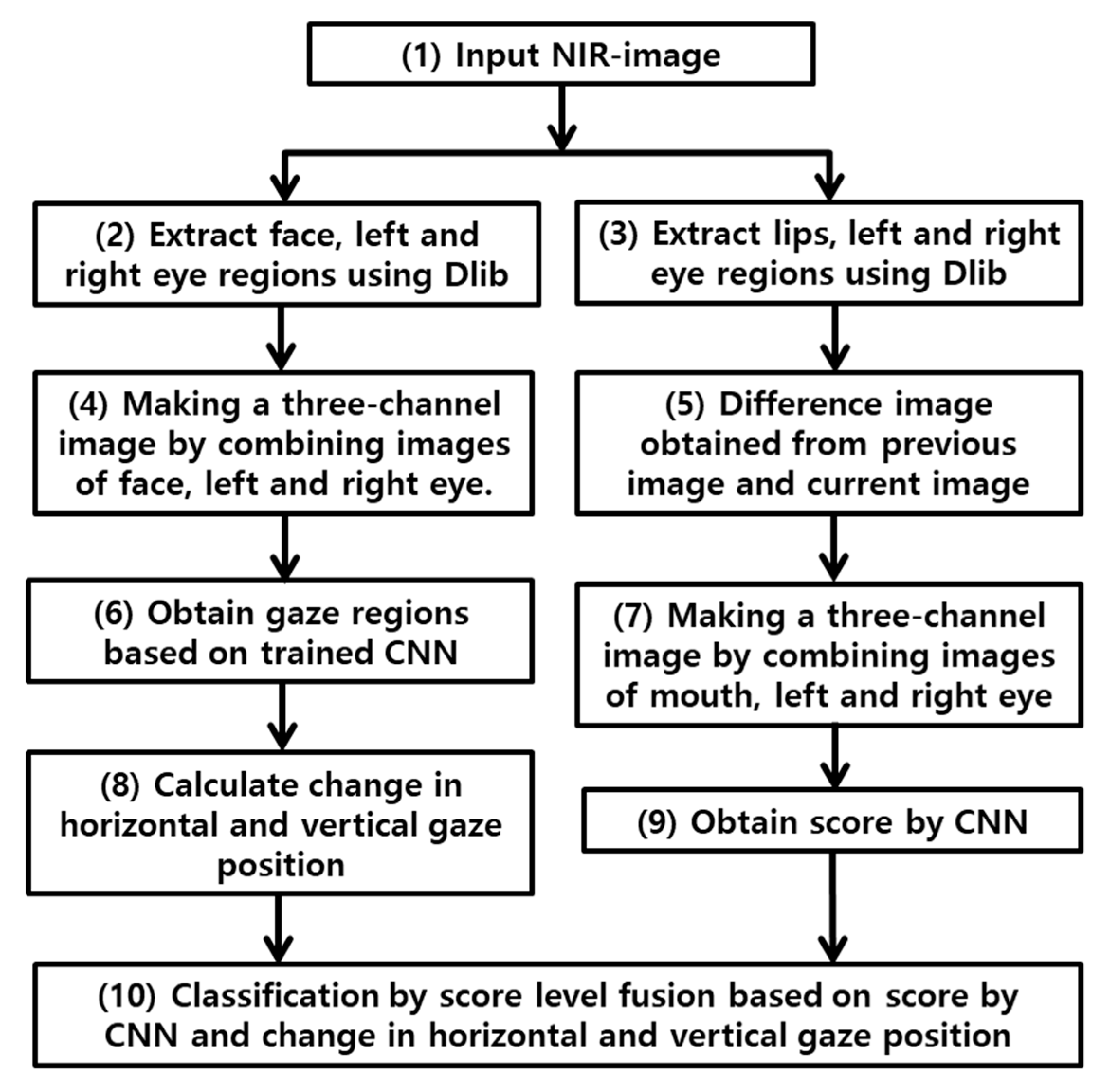
Figure 1. Flowchart of proposed method.
Remotesensing 12 00587 g001
Figure 2. Experimental environment and proposed prototype for driving behavior classification.
Remotesensing 12 00587 g002
Figure 3. Examples of the captured images of near-infrared (NIR) camera.
Remotesensing 12 00587 g003
Figure 4. Examples of detected facial feature points and their corresponding index numbers.
Remotesensing 12 00587 g004
Figure 5. 25 gaze regions defined for training on the 24-inches monitor screen.
Remotesensing 12 00587 g005
Figure 6. Gaze change obtained by (a) Defining region of interest (ROI) on original image based on facial landmarks. (b) Three channel image obtained by combining left eye, right eye, and combined left and right eye.
Remotesensing 12 00587 g006aRemotesensing 12 00587 g006b
Figure 7. NIR image for showing facial emotions: (a) selected ROIs for emotions; (b) for facial emotions difference image generation.
Remotesensing 12 00587 g007aRemotesensing 12 00587 g007b
Figure 8. Block diagram of proposed convolutional neural network (CNN) structure for driver’s behavior classification.
Remotesensing 12 00587 g008
Figure 9. CNN Architectures used for classifying driving behavior.
Remotesensing 12 00587 g009
Figure 10. Steps followed during experimental procedure. Normal and smooth driving images are collected while operating euro truck simulator 2 [58] and need for speed [57] simulators respectively.
Remotesensing 12 00587 g010
Figure 11. Graphs of mean and standard deviation for three features between normal and aggressive driving: (a) Horizontal gaze change, (b) Vertical gaze change, and (c) Change in facial emotions.
Remotesensing 12 00587 g011aRemotesensing 12 00587 g011b
Figure 12. Accuracy and loss curves of training according to the number of epoch (a) Proposed method (b) AlexNet method.
Remotesensing 12 00587 g012
Figure 13. Examples of the facial images from Open database: (a) normal emotion; (b) aggressive emotion.
Remotesensing 12 00587 g013aRemotesensing 12 00587 g013b
Figure 14. Receiver operating characteristic (ROC) curves of proposed method and its comparison with previous methods.
Remotesensing 12 00587 g014
Figure 15. ROC curves of proposed method and its comparison with previous methods on Open database [69].
Remotesensing 12 00587 g015
Table 1. Comparison between the proposed and previous researches on driver’s behavior classification.
CategoryMethodsAdvantageDisadvantage
Non-visual behavior based methods Bio-signal-based method [10,11,12,13]Driver’s emotions or exhaustion is measured using different bio-electric signals such as ECG, EEG - Useful to detect physiological changes in the form of bio-signals
- Bio-signals can be used as an input data for detecting emotions
- Bio-electric signals are high-speed signals that cannot be detected by naked eyes
- Bio-signal sensors are expensive and not feasible for commercial use
- Possibility of detachment from driver’s body
- Psychological discomfort for the user
Voice-based method [14,15,16,17]Driver’s voice or car-voice interaction was examined to analyze driver’s emotion - Sensors used for this method are very cheap - Performance of system is badly affected by surrounding noise
Gyro-sensor and accelerometer-based method [3,4,18,19,20,21,22,23] Driver’s driving behavior is detected - Highly portable as accelerometer and gyro-sensor in a smart phone can be used for this method
- No extra device needs to be purchased or installed
- Close correlation with aggressive driving as vehicles motion can be observed easily
- Method is inapplicable in areas out of coverage of GPS systems
- Performance is highly dependent on the efficiency of GPS receiver
- Driving on mountainous roads can be misclassified as aggressive driving
Visual-behavior based methodsMulti cameras-based system [25,26,27,28,29]Fuse different information from eyes and head pose from more than one camera sensor for analyzing drivers - Higher reliability due to less possibility of invisible face regions by wide range of multiple cameras
- Reliability is higher due to multiple sources of information
- Computational complexity is higher as compared to single camera-based methods
- Only applicable for the characteristics visible by naked eye
Single camera-based systemsVisible light camera-based systems [30,31,32,33]Driver’s behavior detection using visible light camera - Normal common purpose camera is used- In efficient in dark environment especially during night or passing through a tunnel
- Higher possibility of invisible face regions that can reversely affect the efficiency of system
Thermal camera-based systems [36,37]Driver’s facial emotion recognition using thermal camera - Precise physical signals for particular emotion can be detected that is not possible with visible light or NIR camera
- No special illuminator is required to operate at night
- Efficiency for detecting facial emotions is lower as compared to visible light and NIR camera
- Thermal cameras are expensive as compared to others
NIR camera-based systemsDriver’s vigilance monitoring using NIR camera [35]- Fuzzy system is used for PERCLOS to detect vigilance level
- No intensive training is required
- Work with the fatigue level of the driver only
- System does not work well at day time and with driver’s wearing glasses
Single NIR camera based driver’s driving behavior classification using change in gaze and facial emotions purely based on CNN (Proposed Method)- NIR camera can efficiently detect facial features as well as gaze information
- An intensively trained CNN is robust to various environmental and driver conditions
- Cheaper system with multiple features
- Only work with the physical characteristics that can be observed with naked eye
- Intensive CNN training is required
Table 2. Configuration of CNN model used in proposed method (CL means convolutional layer).
Layer TypeNumber of FilterSize of Feature MapSize of KernelNumber of StrideNumber of Padding
Image input layer 224 × 224 × 3
Group 1Conv1_1 (1st CL)64224 × 224 × 643 × 31 × 11 × 1
Relu1_1 224 × 224 × 64
Conv1_2 (2nd CL)64224 × 224 × 643 × 31 × 11 × 1
Relu1_2 224 × 224 × 64
Pool11112 × 112 × 642 × 22 × 20 × 0
Group 2Conv2_1 (3rd CL)128112 × 112 × 1283 × 31 × 11 × 1
Relu2_1 112 × 112 × 128
Conv2_2 (4th CL)128112 × 112 × 1283 × 31 × 11 × 1
Relu2_2 112 × 112 × 128
Pool2156 × 56 × 1282 × 22 × 20 × 0
Group 3Conv3_1 (5th CL)25656 × 56 × 2563 × 31 × 11 × 1
Relu3_1 56 × 56 × 256
Conv3_2 (6th CL)25656 × 56 × 2563 × 31 × 11 × 1
Relu3_2 56 × 56 × 256
Conv3_3 (7th CL)25656 × 56 × 2563 × 31 × 11 × 1
Relu3_3 56 × 56 × 256
Pool3128 × 28 × 2562 × 22 × 20 × 0
Group 4Conv4_1 (8th CL)51228 × 28 × 5123 × 31 × 11 × 1
Relu4_1 28 × 28 × 512
Conv4_2 (9th CL)51228 × 28 × 5123 × 31 × 11 × 1
Relu4_2 28 × 28 × 512
Conv4_3 (10th CL)51228 × 28 × 5123 × 31 × 11 × 1
Relu4_3 28 × 28 × 512
Pool4114 × 14 × 5122 × 22 × 20 × 0
Group 5Conv5_1 (11th CL)51214 × 14 × 5123 × 31 × 11 × 1
Relu5_1 14 × 14 × 512
Conv5_2 (12th CL)51214 × 14 × 5123 × 31 × 11 × 1
Relu5_2 14 × 14 × 512
Conv5_3 (13th CL) 51214 × 14 × 5123 × 31 × 11 × 1
Relu5_3 14 × 14 × 512
Pool517 × 7 × 5122 × 22 × 20 × 0
Fc6 (1st FCL) 4096 × 1
Relu6 4096 × 1
Dropout6 4096 × 1
Fc7 (2nd FCL) 4096 × 1
Relu7 4096 × 1
Dropout7 4096 × 1
Fc8 (3rd FCL) 25 × 1(2 × 1)
Softma × layer 25 × 1(2 × 1)
Output layer 25 × 1(2 × 1)
Table 3. Description of training and testing images from DDBC-DB1.
TrainingTesting
Normal DrivingAggressive DrivingNormal DrivingAggressive Driving
1st fold cross validation19,64219,64219,64219,642
2nd fold cross validation19,64219,64219,64219,642
Table 4. p-value, Cohen’s d value, and effect size of five features between normal and aggressive driving.
Change in Horizontal GazeChange in Vertical GazeChange in Facial Emotions
NormalAggressiveNormalAggressiveNormalAggressive
Average0.2630.3990.2930.5010.2360.647
Standard deviation0.0310.0380.0450.0520.0470.055
p-value2.66 × 10−41.44 × 10−43.56 × 10−5
Cohen’s d value3.944.298.06
StrengthLargeLargeLarge
Table 5. Parameters used by our stochastic gradient descent (SGD) method.
Learning Rate Drop Period (Epochs)Learning RateLearning Rate Drop FactorL2 RegularizationMomentumMini-batch Size
200.0010.10.00010.920
Table 6. Classification accuracies by VGG- face 16 model (%).
VGG-16 model (CHG)
ActualPredicted
1st fold2nd foldAverage
AggressiveNormalAggressiveNormalAggressiveNormal
Aggressive71.6728.3373.3126.6972.4927.51
Normal27.7872.2226.3473.6627.0672.94
VGG-16 (CVG)
ActualPredicted
1st fold2nd foldAverage
AggressiveNormalAggressiveNormalAggressiveNormal
Aggressive75.8824.1276.9723.0376.42523.575
Normal24.0275.9877.0722.9350.54549.455
VGG-16 (CFE)
ActualPredicted
1st fold2nd foldAverage
AggressiveNormalAggressiveNormalAggressiveNormal
Aggressive85.4314.5783.9116.0984.6715.33
Normal15.1184.8916.1483.8615.62584.375
Table 7. Equal error rate (%) obtained from feature values through weighted SUM rule.
Change in Horizontal Gaze PositionChange in Vertical Gaze PositionChange in Facial EmotionsEqual Error Rate (%)
0.500.59.4%
00.50.58.6%
0.50.5026.6%
0.330.330.3311.0%
0.30.20.55.8%
0.20.30.53.7%
0.20.20.61.9%
0.210.190.62.3%
0.190.210.61.1%
0.180.220.61.6%
0.150.150.74.7%
optimal weights based on weighted SUM rule are shown in bold.
Table 8. Equal error rate (%) obtained from feature values through weighted PRODUCT rule.
Change in Horizontal Gaze PositionChange in Vertical Gaze PositionChange in Facial EmotionsEqual Error Rate (%)
0.500.510.9%
00.50.59.6%
0.50.5027.2%
0.330.330.3311.2%
0.30.20.57.1%
0.20.30.54.5%
0.20.20.63.3%
0.210.190.63.9%
0.190.210.62.6%
0.180.220.63.1%
0.150.150.76.2%
optimal weights based on weighted PRODUCT rule are shown in bold.
Table 9. Classification accuracies by proposed method, based on score-level fusion (%).
ActualPredicted
1st Fold2nd FoldAverage
AggressiveNormalAggressiveNormalAggressiveNormal
Aggressive99.030.9798.831.1798.931.07
Normal0.9899.021.1598.851.06598.935
Table 10. Classification accuracies by AlexNet model (%).
AlexNet model (CHG)
ActualPredicted
1st fold2nd foldAverage
AggressiveNormalAggressiveNormalAggressiveNormal
Aggressive61.7838.2262.5337.4762.15537.845
Normal39.6660.3438.7761.2339.21560.785
AlexNet model (CVG)
ActualPredicted
1st fold2nd foldAverage
AggressiveNormalAggressiveNormalAggressiveNormal
Aggressive64.935.165.3134.6965.10534.895
Normal35.1664.8434.5365.4734.84565.155
AlexNet model (CFE)
ActualPredicted
1st fold2nd foldAverage
AggressiveNormalAggressiveNormalAggressiveNormal
Aggressive71.3228.6872.127.971.7128.29
Normal28.6371.3728.1571.8528.3971.61
Table 11. Classification accuracies by score level fusion while using the AlexNet model [53] (%).
ActualPredicted
1st Fold2nd FoldAverage
AggressiveNormalAggressiveNormalAggressiveNormal
Aggressive87.6012.4087.2012.8087.4012.60
Normal12.2587.7512.9387.0712.5987.41
Table 12. Classification accuracies of proposed method on Open Database [69] (%).
ActualPredicted
1st Fold2nd FoldAverage
AggressiveNormalAggressiveNormalAggressiveNormal
Aggressive91.368.6489.9210.0890.649.36
Normal8.7791.2310.1789.839.4790.53
Table 13. Classification accuracies of previous method [53] on Open Database [69] (%).
ActualPredicted
1st Fold2nd FoldAverage
AggressiveNormalAggressiveNormalAggressiveNormal
Aggressive75.5824.4276.1523.8575.86524.135
Normal24.2975.7123.1676.8423.72576.275
Table 14. Comparison of PPV, true positive rate (TPR), ACC, and F_score of proposed and previous methods (%).
PPVTPRACCF_Score
Proposed method98.9398.93598.93398.933
Proposed method (open database [69])90.6490.5490.58590.59
AlexNet [53]87.4087.40987.40587.404
AlexNet [53] (open database [69])75.86576.17776.0776.02
MHDM [37]74.5874.64774.62574.614
MHDM [37] (open database [69])64.5163.82163.9764.164