Article

Land-Cover Changes to Surface-Water Buffers in the Midwestern USA: 25 Years of Landsat Data Analyses (1993–2017)

1
Pegasus Technical Services, Inc., c/o U.S. Environmental Protection Agency, Cincinnati, OH 45219, USA
2
Office of Research and Development, U.S. Environmental Protection Agency, Cincinnati, OH 45268, USA
3
National Research Council, c/o U.S. Environmental Protection Agency, Cincinnati, OH 45268, USA
4
Department of Natural Resources and the Environment, University of Connecticut, Storrs, CT 06269, USA
5
Department of Geography, University of Tennessee, Knoxville, TN 37996, USA
*
Author to whom correspondence should be addressed.
Remote Sens. 2020, 12(5), 754; https://doi.org/10.3390/rs12050754
Submission received: 14 January 2020 / Revised: 20 February 2020 / Accepted: 21 February 2020 / Published: 25 February 2020
(This article belongs to the Special Issue Advancements in Remote Sensing of Land Surface Change)

Abstract

:
To understand the timing, extent, and magnitude of land use/land cover (LULC) change in buffer areas surrounding Midwestern US waters, we analyzed the full imagery archive (1982–2017) of three Landsat footprints covering ~100,000 km2. The study area included urbanizing Chicago, Illinois and St. Louis, Missouri regions and agriculturally dominated landscapes (i.e., Peoria, Illinois). The Continuous Change Detection and Classification algorithm identified 1993–2017 LULC change across three Landsat footprints and in 90 m buffers for ~110,000 surface waters; waters were also size-binned into five groups for buffer LULC change analyses. Importantly, buffer-area LULC change magnitude was frequently much greater than footprint-level change. Surface-water extent in buffers increased by 14–35x the footprint rate and forest decreased by 2–9x. Development in buffering areas increased by 2–4x the footprint-rate in Chicago and Peoria area footprints but was similar to the change rate in the St. Louis area footprint. The LULC buffer-area change varied in waterbody size, with the greatest change typically occurring in the smallest waters (e.g., <0.1 ha). These novel analyses suggest that surface-water buffer LULC change is occurring more rapidly than footprint-level change, likely modifying the hydrology, water quality, and biotic integrity of existing water resources, as well as potentially affecting down-gradient, watershed-scale storages and flows of water, solutes, and particulate matter.

Graphical Abstract

1. Introduction

Land use and land cover (LULC) progression in the Midwestern United States (US) has changed from historically widespread tallgrass prairie and forested landscapes to intensively managed agricultural lands and highly developed urban landscapes [1,2,3,4,5]. This massive transformation has made the Midwestern US one of the most agriculturally productive regions of the US, where nine states (Illinois, Indiana, Iowa, Kansas, Minnesota, Missouri, Nebraska, Ohio, and South Dakota) are responsible for 76% of the total US crop production [6]. Similarly, urbanization has altered the landscape; between 1940 and 2000 the number of housing units in the Midwestern US grew by 146%, with much of the urbanization occurring in areas peripheral to the metropolitan centers [7].
However, LULC change such as that experienced in the Midwestern US also dramatically alters local- to continental-scale landscape structure, function, connectivity, productivity, and processes [8]. Specific to aquatic resources, research has demonstrated that LULC change affects hydrological functions, including stream discharge [9], peak flows [10], surface runoff [11], water levels [12], and sedimentation rates [13,14,15]. The impacts of LULC change at local to regional scales can further affect watershed-scale biogeochemical processing rates, with concomitant impacts on water quality [16]. Loss of “bioreactive” landscape elements [17], such as wetlands and similar waters, and transformation to different LULC types may cumulatively increase nutrient loading to down-gradient systems [4,18,19,20,21,22].
The effects of anthropogenic alterations on down-gradient biogeochemical concentrations can vary based on waterbody size classes. For instance, Evenson et al. [22] reported that the removal of smaller water bodies (e.g., drained or filled) across a watershed could substantially alter watershed-scale water residence times, which is also likely to affect biogeochemical processing rates. In a literature review of over 600 papers, Cheng and Basu [23] determined that smaller water bodies are more biogeochemically reactive than larger systems. Van Meter and Basu [24], Serran and Creed [25], and Creed et al. [19] have reported that small aquatic systems, such as wetlands, are more likely to experience LULC change (i.e., be hydrologically altered or destroyed), thereby disproportionately affecting watershed-scale hydrological characteristics and biogeochemical processing rates.
Modifications to the areas buffering surface waters can also have profound impacts on the water quantity and quality in a given water body [13,14,26,27,28]. Buffers affect water quality and quantity through energy dissipation and the physical settling of entrained particles. Furthermore, settled particles and solutes can undergo biogeochemical processing in areas buffering water bodies [29,30]. Hence, changes to the buffers (e.g., width, structure) can harbinger state changes affecting aquatic resources [26,31,32], as well as affecting the condition of downstream systems [8].
Remotely sensed LULC change data over time provide informative LULC analyses and syntheses useful for managing watersheds and the water bodies of all sizes that remain therein. However, these analyses tend to focus on gross image-wide changes rather than on the effects of LULC change in areas buffering surface-water bodies [26]. Thus, the signal of LULC change in buffering areas may be lost in the “noise” of LULC change occurring elsewhere across the broader landscape. This signal dampening affects both how we quantify the functions and ecosystem services provided by areas buffering the remaining surface water resources (e.g., [8]) and how shifting LULC changes affect these waters themselves (e.g., [26]). Research advances are therefore needed to understand how—and to what extent—surface water buffers are modified in the broader landscape mosaic of LULC changes.
To address these research gaps, we conducted an analysis of temporally continuous LULC change across a 25 year time period in the Midwestern US. The analysis covers three Landsat footprints including the developing urban lands of Chicago, Illinois, and St. Louis, Missouri, as well as the predominantly agricultural areas surrounding the smaller urban center of Peoria, Illinois. We explored not only 25 consecutive years of footprint-wide change, but also analyzed changes to buffers surrounding different surface-water body size classes. Specifically, we sought to answer the following research questions:
  • What is the magnitude, spatial distribution, and annual rate of LULC change across three Landsat footprints (nearly 100,000 km2) of the Midwestern US?
  • How has LULC change occurred over time in buffers surrounding different water body sizes within the three study areas?
We hypothesized that urbanizing trends would continue apace, and hence LULC change would be greatest in the urban-dominated Landsat footprints (i.e., Chicago, Illinois, and St. Louis, Missouri; [33]). As smaller water bodies are more frequently altered as a result of landscape drainage and filling [13,19], we further expected that the smallest waters in our study, those < 0.1 ha in area, would experience the greatest LULC change in their peripheral buffers. We conducted our analysis using the Continuous Change Detection and Classification algorithm (CCDC, [34,35]) and ~1750 Landsat images for our three study areas, incorporating 35 years of data.

2. Materials and Methods
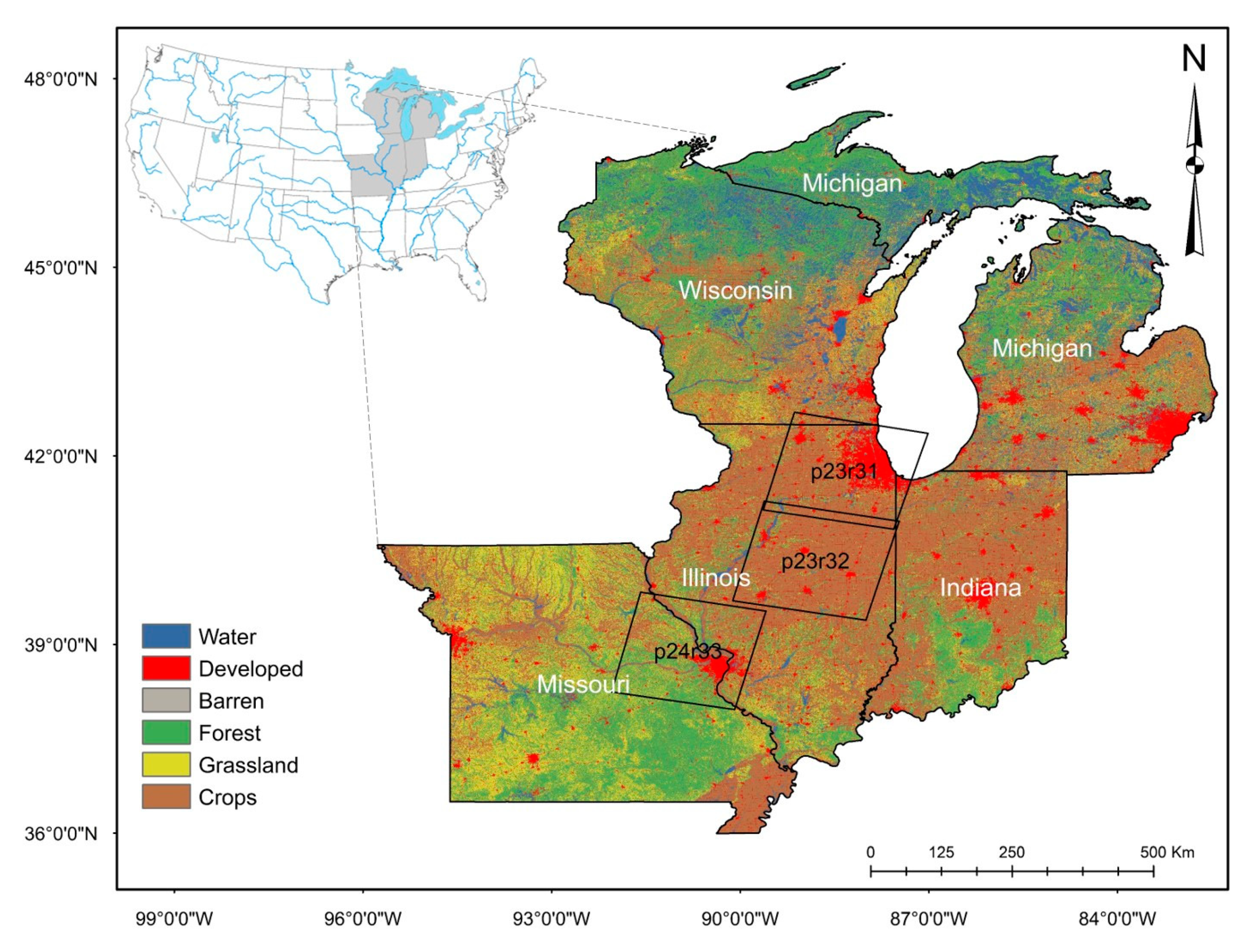
2.1. Study Area

The Midwestern US comprises ~25% of the conterminous US by land area and contains 22% of the nation’s population [36]. The regional climate consists of cold and long winters, with wet springs and temperate summers [37]. However, global climate change models predict warmer and wetter fall-through-spring seasons, with notably drier summer months [38]. The study area is almost entirely in the Major Land Resource Area “Central Feed Grains and Livestock Region” [37] and has level to gently sloping landscapes, much of which consist of the formerly glaciated plains. Our Midwestern study area (Figure 1) includes three Landsat footprints (World Reference System path (p) and row (r) of p23r31, p23r32, and p24r33). The area represented by the three Landsat footprints has both major agricultural production zones and dense population centers [6,7]. As a result, approximately 85% of the pre-European settlement wetlands and similar waters have been lost from the region to agricultural drainage and urban development [39,40]. The urban centers include the cities of Chicago (Illinois) and St. Louis (Missouri) in p23r31 and p24r33, respectively, as well as smaller urban centers in p23r32 (e.g., the Illinois cities of Peoria, Bloomington, Champaign, Decatur, and Springfield). For simplicity, we will hereafter refer to the footprints, from north to south, as Chicago for p23r31, Peoria for p23r32, and St. Louis for p24r33.

2.2. Data Acquisition and Preprocessing

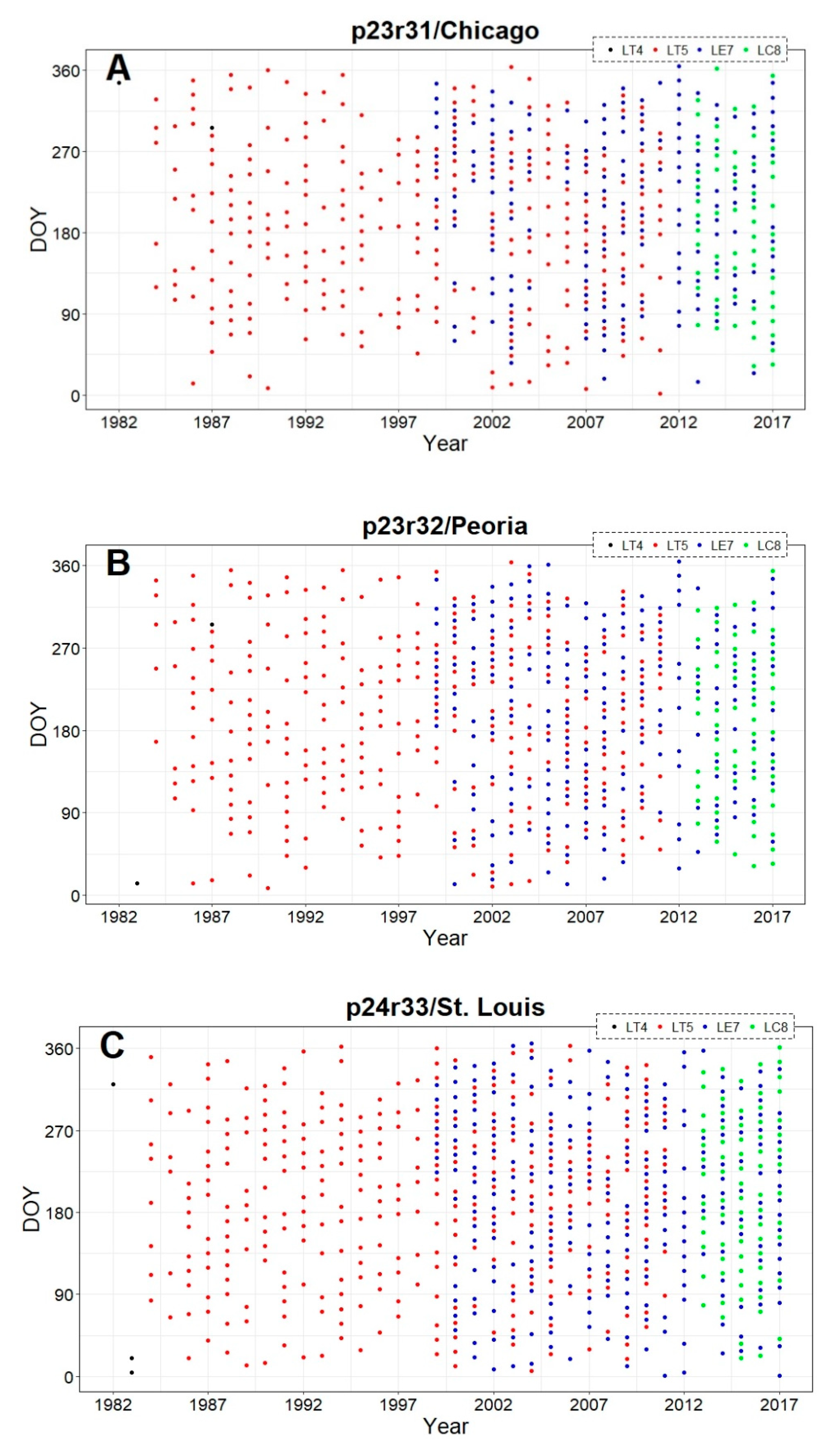
2.2.1. Landsat Data Downloading and Preprocessing

We downloaded geometrically and atmospherically corrected (i.e., USGS “Level 1T”) Landsat 4 and 5 Thematic Mapper (TM), Landsat 7 Enhanced Thematic Mapper Plus (ETM+), and Landsat 8 Operational Land Imager (OLI) data, including all imagery with ≤ 80% cloud-coverage by scene area from the United States Geological Survey-Earth Resources Observation and Science online portal [42,43]. We downloaded a total of 1749 images for the Chicago, Peoria, and St. Louis footprints covering the period 1982-2017, distributed evenly across the years and seasons (Figure 2A–C). We converted raw digital numbers to surface reflectance (bands 1–5, 7) and brightness/surface temperature (band 6) values using the Landsat Ecosystem Disturbance Adaptive Processing System algorithm [44]. We used the GERSLab [45] preprocessing tool to stack the six spectral bands, one thermal band, and one Landsat Level-1 pixel Quality Assessment (QA) or Landsat C version of Function of Mask band (CFMask, providing information about the quality of the pixels in terms of clouds, cloud shadows and snow contaminations [46,47,48]), for the analyses described below.

2.2.2. Land Cover Data Downloading and Processing

We acquired thematic land cover classification maps from the National Land Cover Dataset (NLCD) for 2001, 2006 and 2011 from the USGS portal [43]. We used the 2001 NLCD in the land cover classification, described in Section 2.3, and compared our classification with the three NLCD products, described in Section 2.3.3. The NLCD maps were cropped to the Landsat footprint boundary and re-projected to a common coordinate system (WGS 1984, UTM Zones 15N for St. Louis and 16N for Chicago and Peoria).

2.3. Change Detection Model Implementation and Assessment

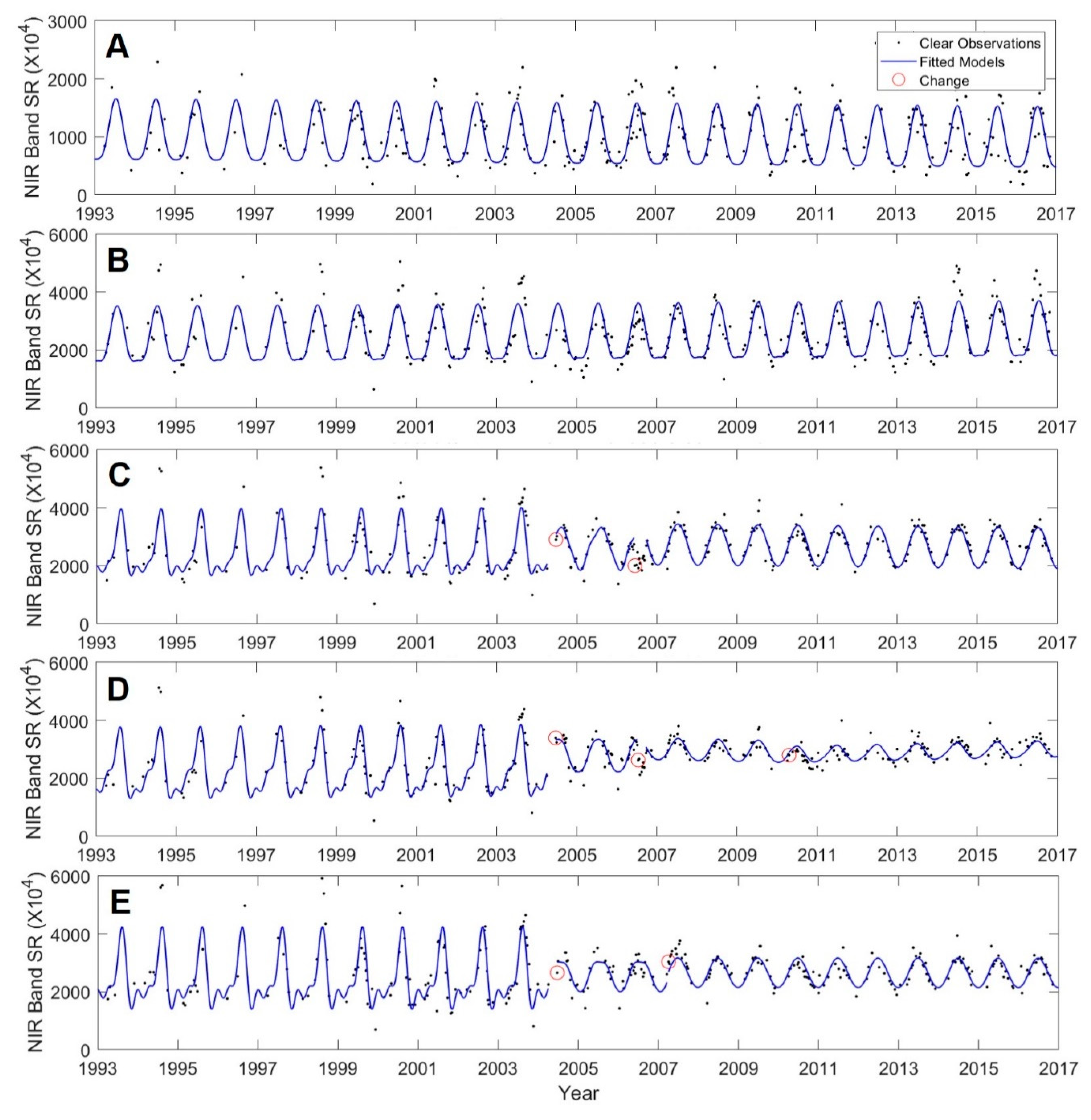
2.3.1. Continuous Change Detection and Classification (CCDC) algorithm

We analyzed regional time-series LULC change analysis using CCDC, which uses the Robust Iteratively Reweighting Least Squares (RIRLS) method to iteratively fit observed data to the LULC dynamic time-series model that incorporates seasonality, trend (for gradual changes), and breaks (for abrupt changes) [34]. We used CCDC version 13.01 (64-bit Linux-machine version) downloaded from Global Environmental Remote Sensing (GERS) Laboratory [45]. The model identifies breaks or transitions using a data-driven thresholding approach on the included Landsat bands [34]. Breaks or changes are identified in CCDC when the spectral signature deviates from the fitted model predictions in consecutive dates of images [34,49]. Further CCDC application fundamentals and details of its implementation can be found in Zhu and Woodcock [34].

2.3.2. Random Forest Training and Classification

We classified the CCDC model output data with version 1.02 of the CCDC Assistor tool [45] within the CCDC environment using random forest [50]. Inputs to the supervised classification included time-series model coefficients and the root mean square error (RMSE) values used to generate a continuous land cover map of the modeling domain [34]. The 2001 NLCD dataset was used to train the classifier using 20,000 pixels distributed proportionally across the original 15 land-cover classes based on the optimized training data selection strategy [47]. Accordingly, the approach uses 600–8000 pixels per class [47,51].
We subsequently binned the continuous land-cover classification maps produced from the CCDC and the NLCD data into six major land cover types for our analyses (see Figure 1): water (NLCD classes of open water, woody wetlands, emergent herbaceous wetlands), forest (NLCD classes of deciduous forest, evergreen forest, mixed forest, and shrub/scrub), grassland (NLCD classes of grassland/herbaceous, pasture/hay), crops (NLCD class of cultivated crops), developed (NLCD classes of developed—open space, developed—low intensity, developed—medium intensity, developed—high intensity), and barren (NLCD class of barren land—rock/sand/clay).

2.3.3. Classification Agreement with NLCD

We evaluated the spatiotemporal performance of the CCDC algorithm and subsequent random forest classification over time through the generation of both omission and commission error metrics.
We assessed classification correspondence with the 2001, 2006, and 2011 NLCD datasets [52,53,54]. We kept a minimum linear separation distance between any two points of 250 m (a distance selected to decrease autocorrelation potential) that resulted in nearly 238,000 randomly distributed points across the three footprints. We assessed classification agreement by (1) extracting the CCDC-derived class for each pixel using July 1st of each year (thereby avoiding untilled agricultural lands and snow-covered landscapes; [51]), and (2) developing confusion matrices contrasting the CCDC class with 2001, 2006, and 2011 NLCD thematic data that we binned into major land-cover types (described above in 2.3.2).

2.4. Data Analyses

We analyzed the annual LULC change for a 25-year period from 1993–2017 at both the image-scale and within a 90 m buffering distance around surface waters, a distance that approximates a commonly used 100 m buffer for aquatic monitoring and assessments [31,55] and one that seamlessly comports to the 30 m Landsat pixel size. The dataset from the period 1982–1985 was used for model initiation and a six year CCDC output window (1986–1991) was used to identify “waters” from the random forest classification (i.e., including open water, woody wetlands, and emergent herbaceous wetlands, as described above). A conservative rubric was applied, such that a pixel was required to be classified as water in at least five of six years between the period 1986–1991 to be considered “water”; this decreased the likelihood that climatic vagaries and/or mixed-pixel (“edge effects”) would result in a pixel being misidentified as water. We used 1992 imagery for final model initiation and conducted LULC change analyses from the period 1993–2017. Waters ranged in size from a single pixel (0.09 ha) to 58,850 ha in size across the three images. We excluded Lake Michigan, a 4000 km2 water body (the portion within our Chicago footprint), from all analyses of the Chicago footprint.
We calculated the LULC change over 25 years using three approaches: (1) footprint-level time-series LULC change, (2) water body buffer time-series LULC change within 90 m buffers for each footprint, and (3) water body size-class analyses of time-series LULC change within a 90 m water body buffers (i.e., a post-hoc approach analyzing each water body uniquely). We conducted the footprint-scale 90 m assessment by first buffering each water body (as determined above) within a GIS environment. We then identified the corresponding 90 m buffer LULC pixels from the CCDC output for each year using R (using R packages raster, rgdal, rgeos, and sf [56,57,58,59]). For the third analysis, each water body had a unique 90 m buffer, with LULC calculated and exported for analyses. For the last analysis, we calculated the area of each water body within a GIS environment and subsequently analyzed LULC change over time, following Christensen et al. [40], binning surface water features into five size-based categories: (a) < 0.1 ha, (b) 0.1 to < 1.0 ha, (c) 1.0 to < 10.0 ha, (d) 10.0 to < 100.0 ha, and (e) ≥ 100 ha.

3. Results

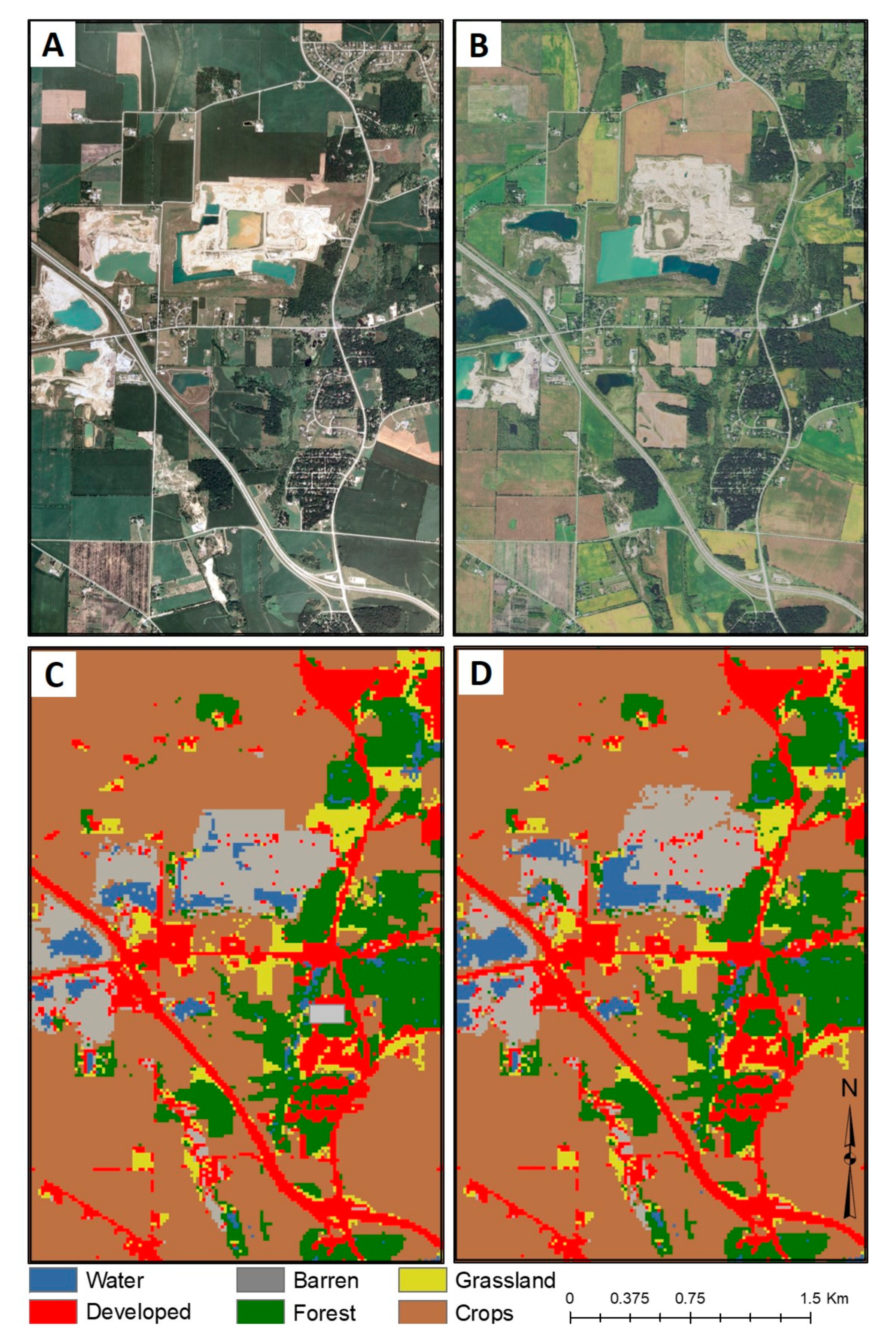
3.1. Thematic Classification Characterization

Confusion matrices (Table 1, Table 2 and Table 3) calculated an overall agreement of 81%–89% across all three footprints and three NLCD datasets (2001, 2006, and 2011). Peoria (footprint p23r32) had the highest overall correspondence of ~89%, whereas Chicago (footprint p23r31) and St. Louis (footprint p24r33) had overall agreements of 84% and 81%, respectively. In general, water, developed, forest, and cropland cover classes were more accurately classified, and grassland and barren classes were more poorly classified. Misclassification errors with grassland and barren classes likely reflect the thresholding process inherent within the NLCD (e.g., barren require <15% vegetation, whereas grasslands require >80% vegetation) and approximate reported regional misclassification errors within the NLCD [41,60]. The small differences in overall agreement between years suggest that the model performed well over time (e.g., overall agreement in Chicago footprint for the three time periods was 84.1% in 2001, 84.0% in 2006, and 83.8% in 2011).

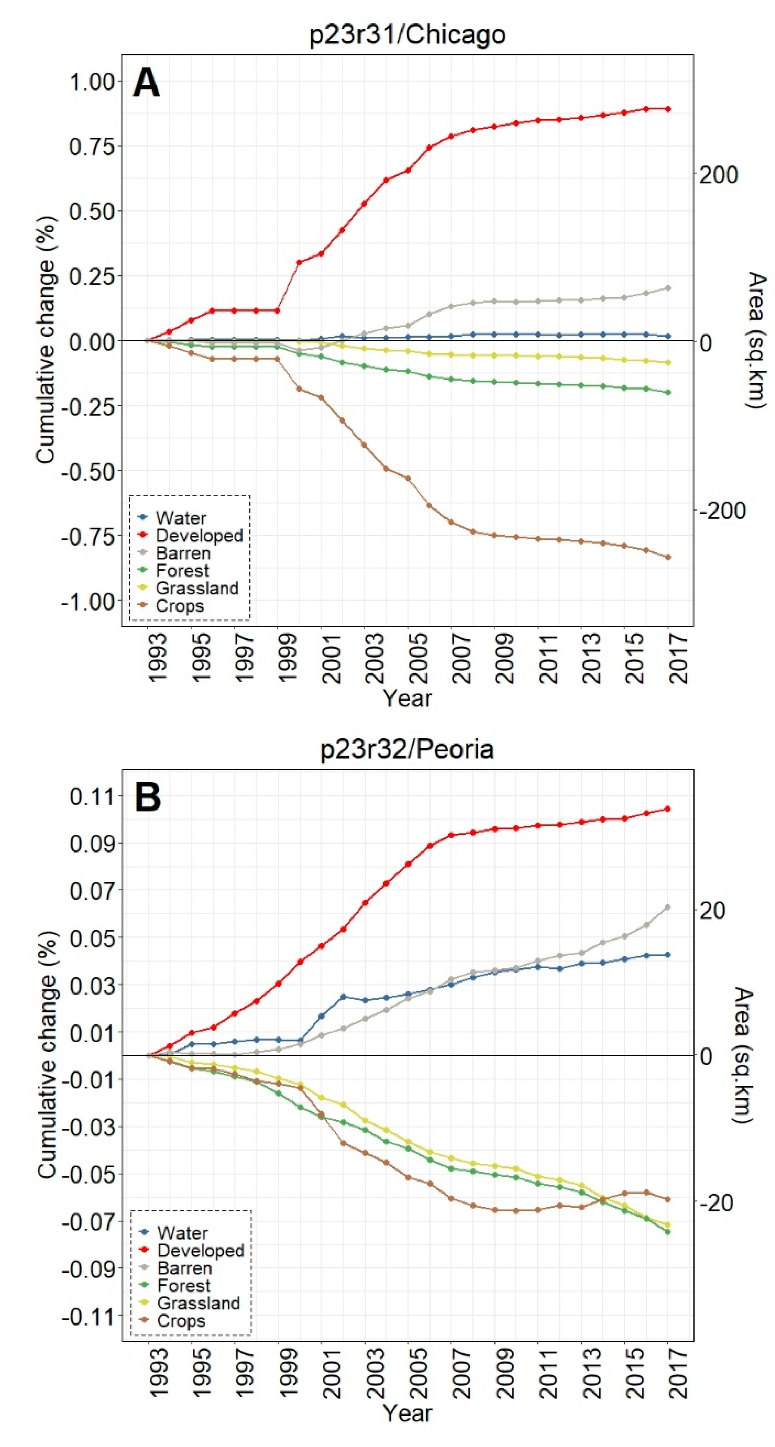
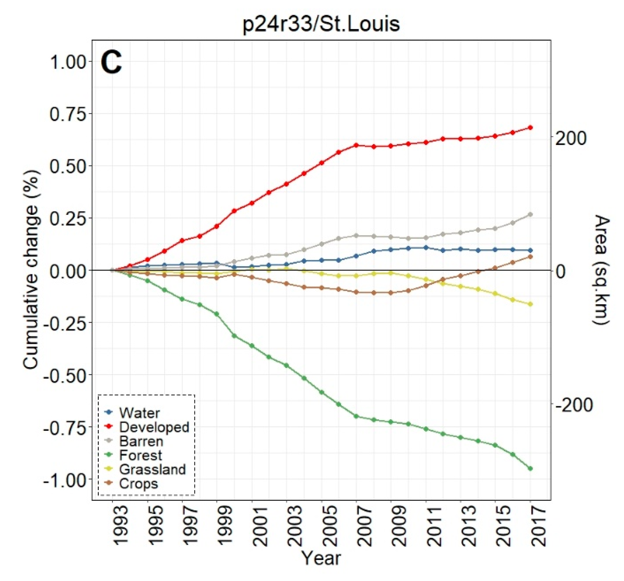
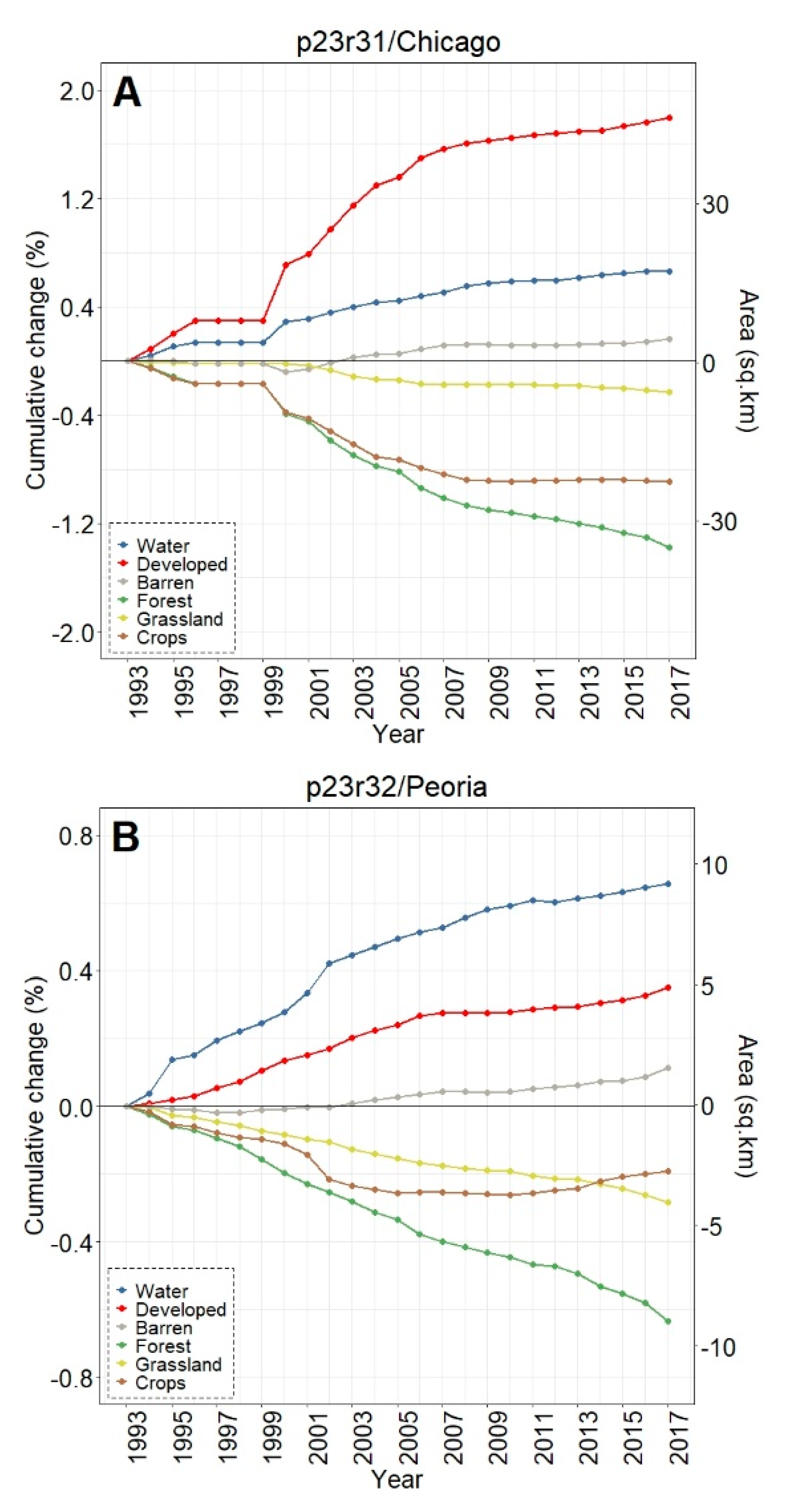
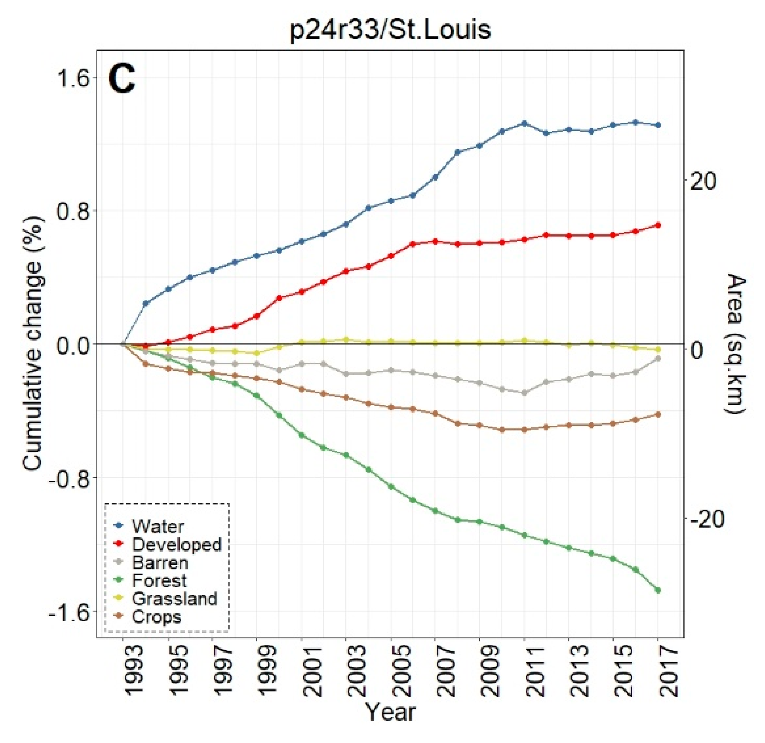
3.2. Spatiotemporal LULC Change Dynamics at Footprint Level

Across all three footprints, developed lands cumulatively increased over 25 years of analyses, while there were concomitant decreases in croplands in the Chicago footprint (Figure 3A), croplands/grasslands/forested lands in the Peoria footprint (Figure 3B), and forested land cover in the St. Louis footprint (Figure 3C). Whilst the percentages of LULC change may be relatively small (e.g., ~1% in 25 years), the actual areal change is substantive—at least for the Chicago and St. Louis footprints. For example, there was a 25 y increase of 280 km2 in developed lands in the Chicago footprint (Figure 3A), while nearly 300 km2 of forested lands in the St. Louis area were converted to other land cover types (see Figure 3C). Developed lands in the Peoria footprint increased ~36 km2; all other changes at the footprint level in the Peoria analyses were <30 km2 (or <0.10%). All three footprints showed increases in water and barren lands. Interestingly, the St. Louis footprint crop LULC change decreased through ~2009 before demonstrating an increased cropland trend around 2009, ultimately resulting in a slight positive increase in croplands (see Figure 3C).
Dynamic change over time is evident in Figure 3A–C using CCDC; Figure 4A–D shows an LULC change in a representative area between two points (2007 and 2015). Figure 5 provides information on the spatiotemporal “year of change”, demonstrating the power of time-series analyses to identify the temporal nature of LULC change.

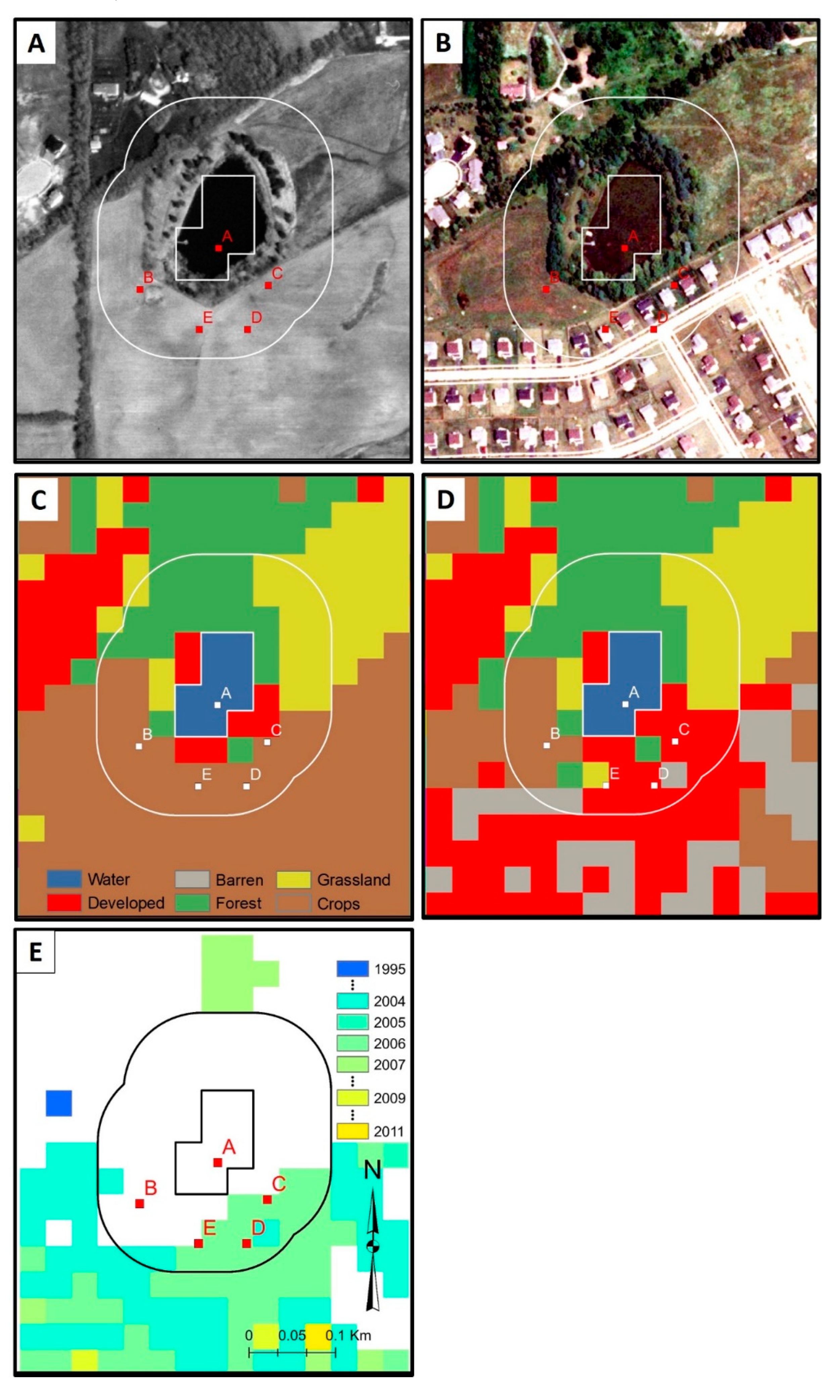
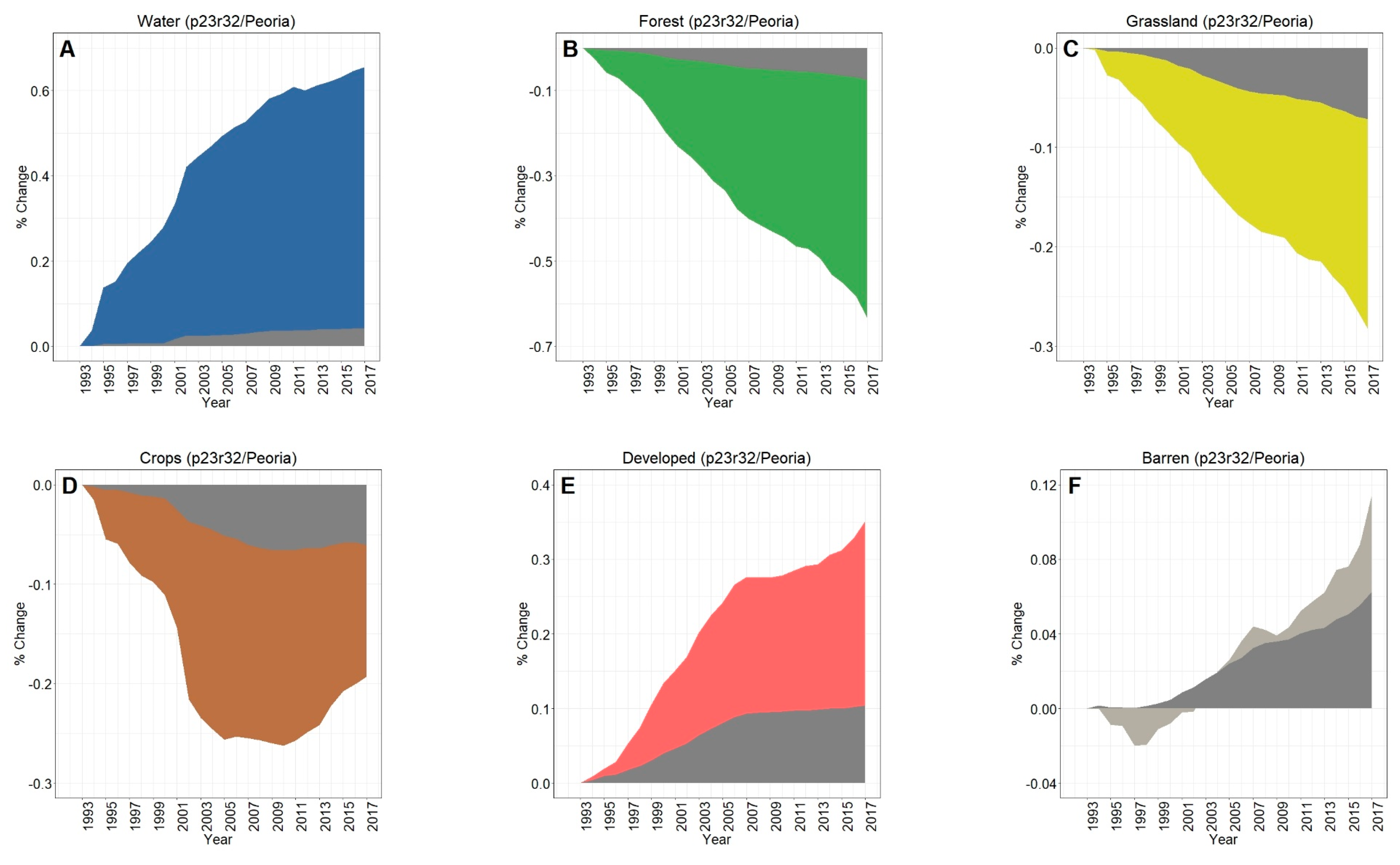
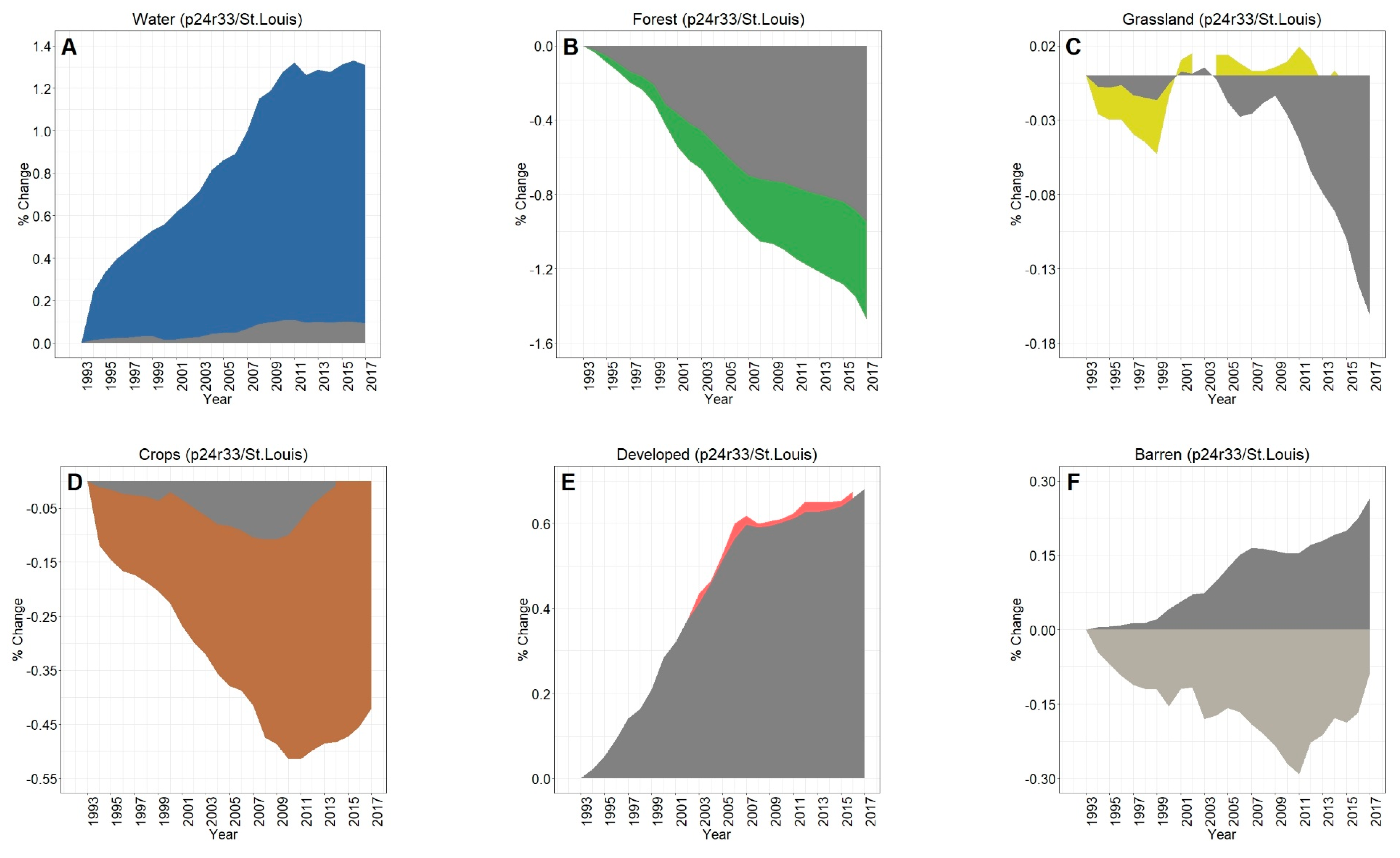
3.3. Spatiotemporal LULC in Surface Water Buffers

3.3.1. LULC Change in Water Body Buffers Compared to Footprint-Scale

We identified 51,619 surface waters in Chicago, 22,186 in Peoria, and 34,475 in St. Louis footprints, covering 3.9%, 2.1%, and 3.3% of each footprint, respectively. Adding the 90 m buffer resulted in the buffer analyses covering approximately 8.2% of Chicago, 4.2% of Peoria, and 6.3% of the St. Louis footprint areas. LULC change over the 25 year horizon occurred in the buffers of 41% of waters in the Chicago-area footprint, 30% in the Peoria-area footprint, and 51% in the St. Louis-area footprint. In Figure 6A–E, LULC change within the buffer surrounding a water body in the Chicago-area footprint is evident, with development encroaching upon the water body (e.g., Figure 6E). Change to the sinusoidal CCDC curves for select points within Figure 6 are presented in Figure 7A–E; indications of LULC change-points across the 25 year time-period for pixels within the areas buffering the water body have evidently occurred ~2004.
The overall LULC change in buffers surrounding water bodies, given in Figure 8A–C, was typically similar in direction to that occurring in footprint-wide analyses (see Figure 3A–C). However, the magnitude of LULC change in the buffering areas was frequently much greater than the footprint-level analyses across all three footprints, as evidenced when contrasting between LULC change in the footprint and the 90 m surface water buffer for Chicago (Figure 9A–F), Peoria (Figure 10A–F), and St. Louis (Figure 11A–F). For example, substantial water expansion occurred in the Chicago study area buffers at 35 times (35x) the relative footprint-wide rate (0.66% versus 0.02% over 25 years, see Figure 9A). Areas buffering surface waters in the Chicago footprint followed the image-wide trend of increased LULC development over 25 years, yet buffer increases were double the image-wide proportional change (1.8% increase compared to ~0.9% increase, respectively (see Figure 9E)). Over the 25 years of Chicago footprint analyses, forests and grasslands buffering surface waters changed at faster rates (decreasing at ~7x and ~3x, respectively; see Figure 9B–C) relative to the full footprint.
Twenty-five years of Peoria imagery analyses follow a similar pattern, with a nearly 15x increase in surface water into the buffers relative to the footprint-wide analyses (see Figure 10A). Developed lands increased 4x in the Peoria buffers relative to the full footprint-wide change (0.35% versus 0.10%, see Figure 10E), whereas there was a 9x decrease in forested lands (−0.63% versus −0.07%, see Figure 10B) and a 4x decrease in grasslands (−0.28% versus −0.07%, see Figure 10C). This footprint also had an increase in barren lands within the buffers 2x greater than the footprint-wide change (0.12% versus 0.06%, see Figure 10F).
Like Chicago and Peoria, surface waters in the St. Louis footprint buffers increased markedly, 14x greater than the entire footprint (1.31% versus 0.09%, see Figure 11A). St. Louis imagery analyses demonstrated no meaningful differences in developed lands between the buffered and footprint-wide changes over 25 years (0.71% versus 0.68%, respectively, see Figure 11E). Forested lands buffering waters were converted at ~2x the footprint rate (−1.48% versus −0.95% over 25 years, see Figure 11B). Grasslands buffering surface waters were converted more slowly than grassland change across the St. Louis footprint, at 1/5 the LULC change rate (−0.03% in the buffer versus −0.16% at the footprint-level over 25 years, see Figure 11C). Croplands in the buffer and footprint-wide followed a similar decreasing trend through ~2008, increasing from that point such that by 2017 there was a slight increase (0.07%) in footprint-wide cropland abundance (though still a substantial decrease in buffer-area croplands (−0.42%; see Figure 11D)). Barren lands decreased in buffering areas (−0.09%) but switched direction and increased at the footprint-scale (0.27%; see Figure 11F).
Changes in lands buffering surface waters were typically not a one-off event. Of the water buffers that changed LULC during our study period, two changes was the mode within each of the three footprints (e.g., from forest to barren, then from barren to developed); 39.6% of Chicago, 46.2% of Peoria, and 38.6% of St. Louis buffers changed LULC twice during the study period. Three or more cumulative LULC buffering area changes occurred in Chicago (57.5%), Peoria (51.6%), and St. Louis (57.9%) across the 25 year analysis.

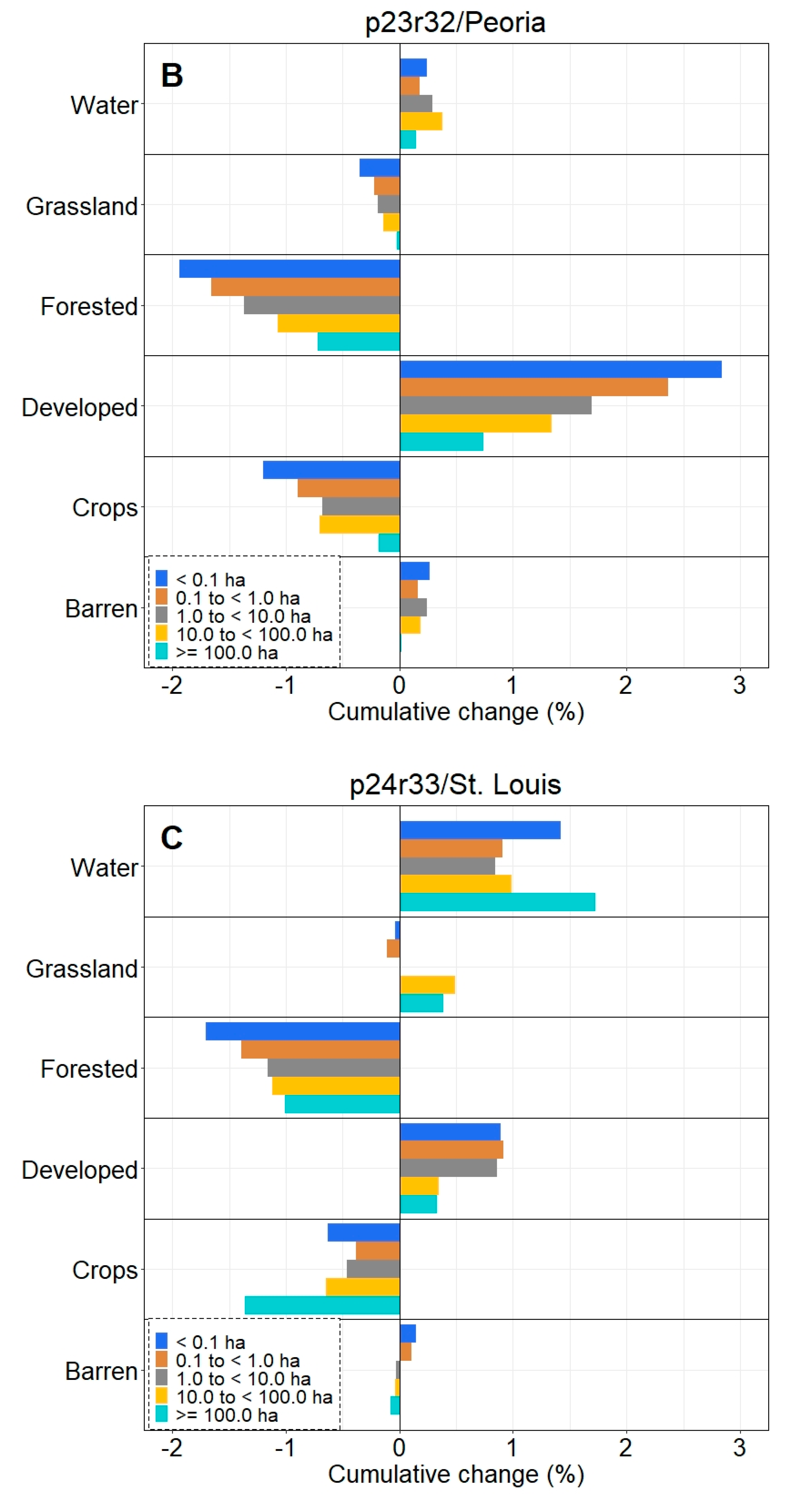
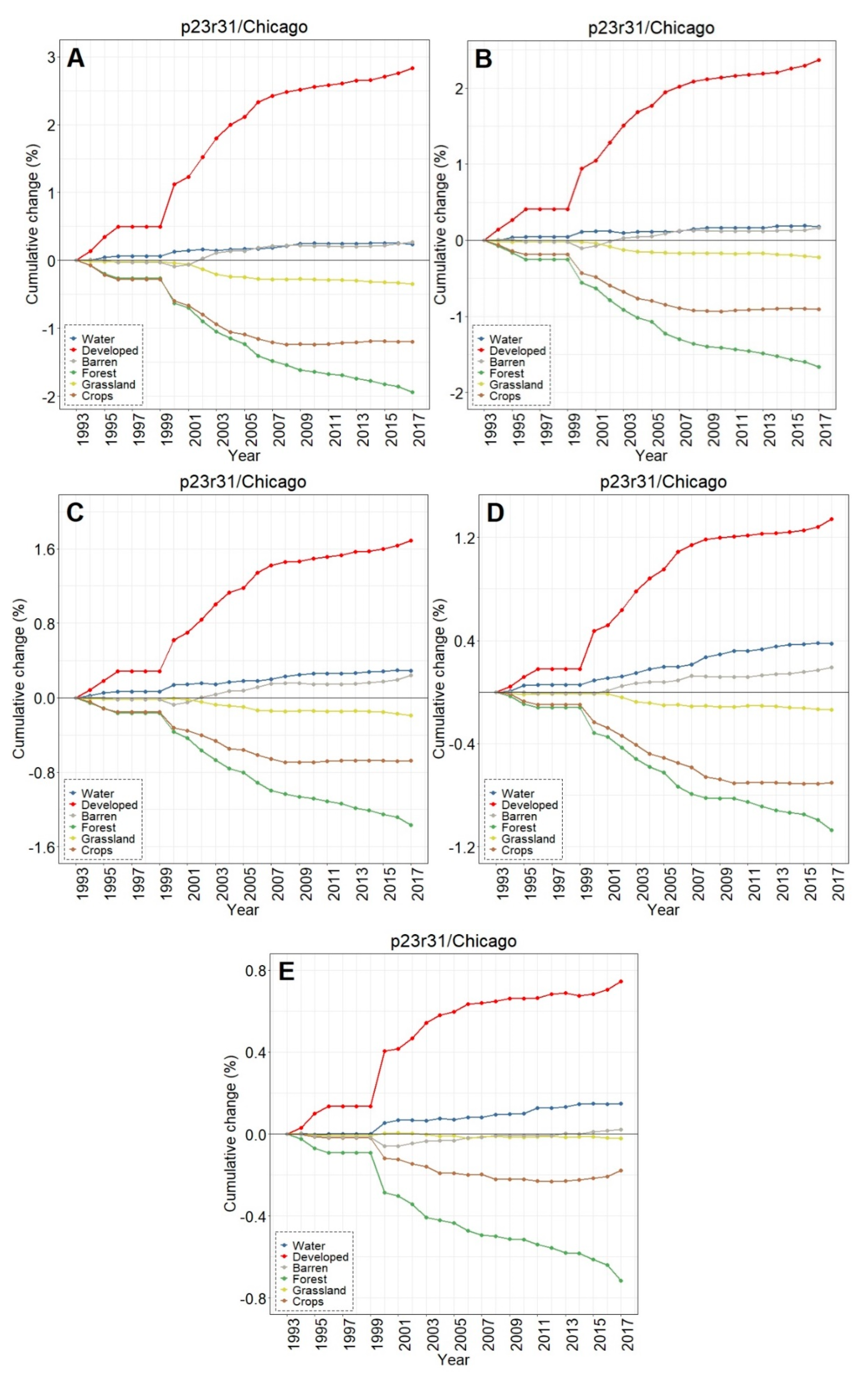
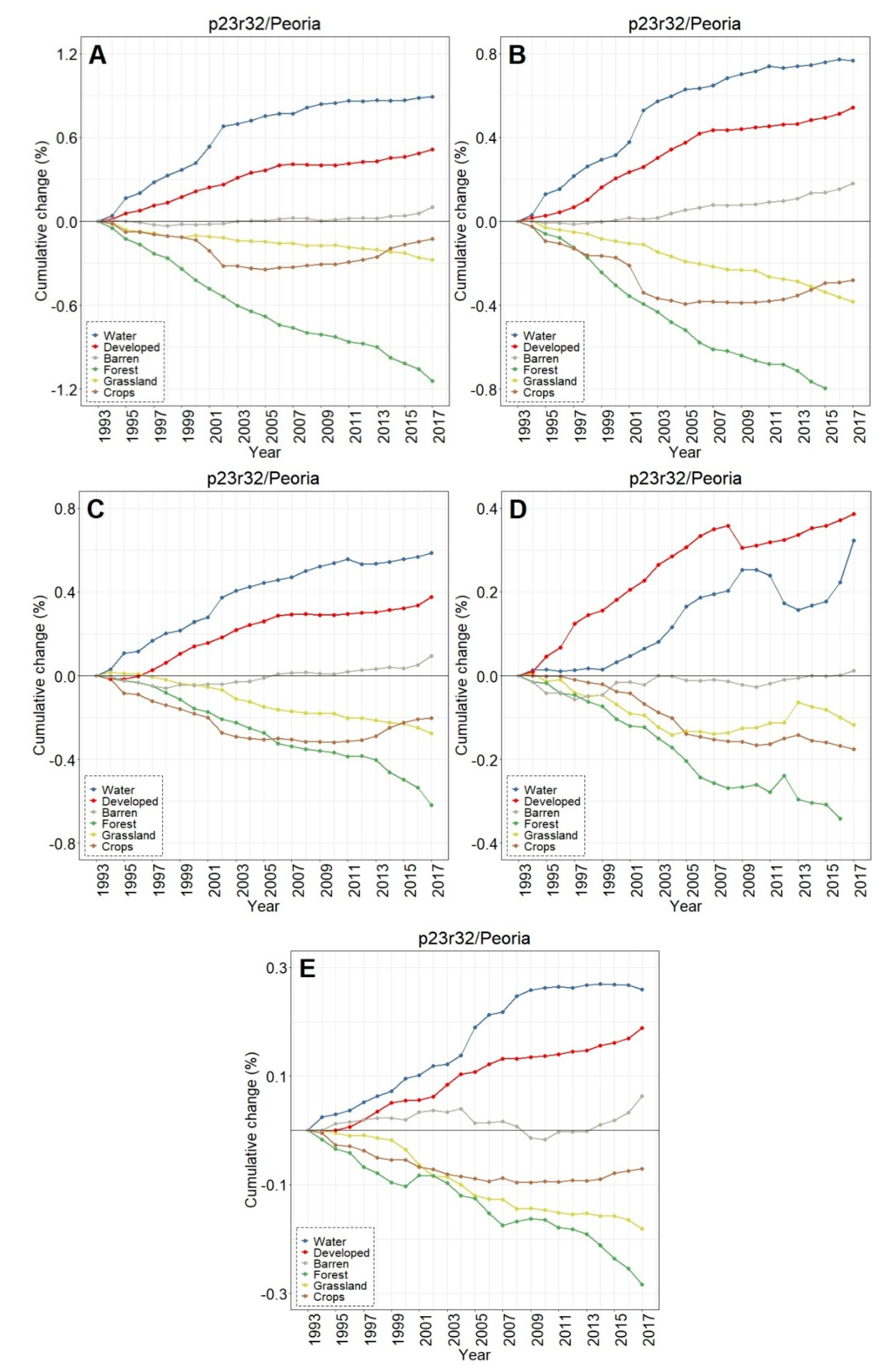
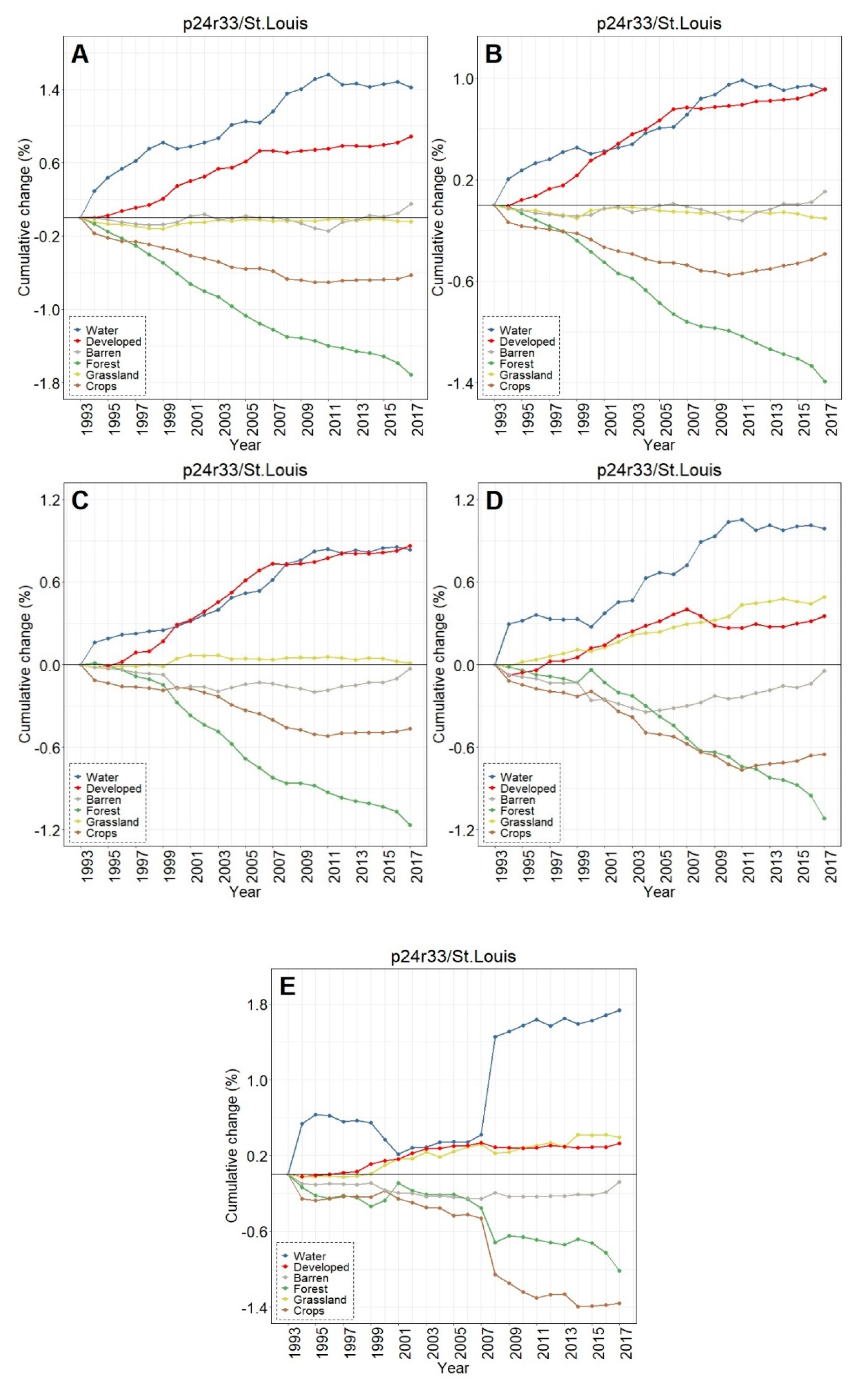
3.3.2. LULC Change in Buffers by Water Body Sizes

The vast majority of extant surface waters across all three Landsat footprints were <1.0 ha in size (87% of 51,619 surface waters in Chicago, 85% of 22,186 surface waters in Peoria, 88% of 34,475 surface waters in St. Louis). The smallest size class (< 0.1 ha) was the mode in Chicago (44%) though the second-most abundant size class in Peoria (40%) and St. Louis (42%), after waters between 0.1 to <1.0 ha in both areas (Table 4). The largest waters, those ≥ 100 ha (and excluding Lake Michigan in the Chicago footprint), represented 0.1%–0.2% of the extant surface waters in our study areas.
Buffer LULC change differed substantially depending on the size of the water body being buffered (Figure 12A–C). In the Chicago footprint, developed, croplands, grasslands, and forested lands all had the same approximate stair-step LULC-change trend over 25 y (Figure 12A), with the largest LULC changes in the buffers surrounding the smallest waters and the least change around the largest water bodies. For instance, there was a cumulative 25 y increase in developed lands that was greatest in the buffers surrounding the smallest waters (<0.1 ha, 2.84%) followed by the second-smallest (0.1 to <1.0 ha, 2.37%), etc. This trend held for decreases in the abundance of forested lands and grasslands; croplands followed suit, but no meaningful difference was discerned between changes in buffers surrounding waters of 1.0 to <10.0 ha (−0.68%) and 10.0 to <100.0 ha (−0.70%). Water (and barren lands) increased over the course of 25 y without any apparent trend associated with size classes in the Chicago footprint. Exploring the temporal nature of the LULC changes, there was a substantive increase in water (in particular), as well as forested and crops around 1999 across all five size classes (Figure 13A–E).
The smallest water bodies in Peoria had the largest LULC increase in percentage water, followed in stair-step fashion by the second smallest, etc. (see Figure 12B). The abundance of forested lands decreased in a similar manner, with the greatest change in the areas surrounding the smallest waterbodies and the least change in the largest waterbodies. Developed lands in buffers increased in tandem between waterbodies <1.0 ha (0.52–0.55%) and those between 1.0 ha and <100.0 ha (0.38–0.39%) before halving to 0.18% in the largest waters. Croplands, grasslands, and barren lands did not evince any particular manner of change when contrasted with the binned data. There was a decrease in grasslands in the buffers surrounding the largest waters, starting in 1999, while LULC change in the remaining four size classes demonstrated a more consistent change-trajectory over the 25 y period of record in the Peoria footprint (Figure 14A–E). The largest water bodies (>100.0 ha) in the St. Louis footprint experienced the greatest increase in water in the buffering areas (1.73%), followed by the smallest water bodies (1.42%); the remaining size classes vacillated between 0.84%–0.99% increases (see Figure 12C). The two largest classes, those water bodies ≥10.0 ha and larger, demonstrated the greatest decrease in croplands in the buffering areas (−0.65% to −1.36%). The smaller water bodies (i.e., the three binned classes <10.0 ha) had the greatest increases in developed lands in the St. Louis footprint (0.86%–0.92%). Forested lands in the St. Louis footprint decreased in a stair-step manner as in Peoria and Chicago, with the greatest decrease in the buffers surrounding the smallest water bodies (<0.1 ha, −1.71%) followed by the next size class (0.1 to <1.0 ha) and so on. CCDC analyses indicated a substantive increase in the abundance of water in areas buffering the largest systems, those ≥ 100 ha, in 2007 (Figure 15A–E).

4. Discussion

Dynamics of LULC Change in the Midwestern US

The progression of LULC change across the Midwestern US has resulted in significant advances in agricultural production, industrialization, and urban growth. Analyzed through the lens of an entire Landsat footprint (or, here, three such footprints), the last 25 years have seen a decrease in forested and agricultural (crop) lands and an increase in developed lands, especially in the urbanizing exurbs of Chicago and St. Louis. This finding follows similar results from LULC change analyses at the conterminous US-scale [62], as well as more regional analyses (e.g., [63,64]). For instance, Maimaitijiang et al. [54] analyzed LULC change in the St. Louis metropolitan area (not a full Landsat footprint) between 1972–2010 at five time-steps (i.e., 1972, 1982, 1990, 2000, and 2010) and reported increases in developed lands and decreases in croplands and grasslands (similar to our study). However, using time-series analyses through CCDC, we found a substantive uptick in agricultural lands around 2010, when their study period ended and near the onset of a near doubling in the per-bushel price of corn [65]. The authors also found decreases in the forested lands and increases in water extent in the greater St. Louis region through 2010 [54], and the change continued apace through to the end of our study in 2017.
Novel to our study of three Landsat footprints covering nearly 100,000 km2 is the finding that development is particularly prevalent in the buffered areas surrounding existing small waterbodies—the wetlands, ponds, and lakes providing numerous ecosystem services [19,23,66,67,68]. Across all three Landsat images, the smallest water bodies (i.e., those < 1.0 ha) experienced the greatest change in the lands buffering them from terrestrial inputs. Furthermore, these changes in the buffers surrounding water bodies occurred at rates substantially faster than the prevailing footprint-wide Landsat changes. Specifically, buffered areas in the Chicago and Peoria footprints converted to developed lands at two to four times the footprint-wide rate, and forested and grasslands decreased between seven to nine times faster (for forested) and three to four times faster (for grasslands) in buffers than occurred across the footprint. Lands buffering water bodies in the St. Louis footprint analysis changed, though at rates similar to the footprint-wide change, with no discernable differences between development (increasing 0.69% in the footprint-wide analysis and 0.72% in the buffers) and relatively minor changes in the forested land conversion in the buffers (~2x the footprint-wide change). Nevertheless, the smaller water bodies in St. Louis (i.e., those <10.0 ha) experienced a higher developed land conversion rate (0.86%-0.92% over 25 years) than the footprint-wide analyses (0.72% over 25 years).
Conversion of the lands buffering water bodies may have profound effects on the waters themselves [29,32,69,70]. For instance, Christensen et al. [71] reported that lands buffering stream networks in agricultural landscapes removed 52% of the edge-of-field nitrogen, a major determinant of aquatic resource eutrophication (e.g., [72]). The buffering areas can filter out pollutants and sediments that affect water quality and aquatic biota, as well as modify temperatures in aquatic systems through shading mechanisms. Supporting the maintenance of aquatic buffers, Wahl et al. [73] found the greatest abundance of pollution-sensitive insect orders Ephemeroptera, Plecoptera, and Trichoptera (“EPT”) in aquatic networks with forested buffers and the lowest in agriculturally cultivated or urban-developed catchments (i.e., those without buffers). Biogeochemical cycling rates within water bodies respond to the differences in loading rates, which can vary depending on the surrounding land uses [70]. Furthermore, the conversion of lands buffering water bodies can increase sedimentation rates and decrease hydroperiods, which can threaten migratory waterfowl and other organisms [26,74,75,76,77].
However, while the conversion and development of lands buffering water bodies occurred at elevated rates vis-à-vis the Landsat footprint (in Chicago and Peoria footprints in particular), this study found a substantial expansion of existing waters into the buffering lands across all three footprints analyzed (i.e., buffer expansion rates ranging from 14–35x footprint-wide rates). The smallest waters in Peoria (<0.1 ha) had the greatest expansion, whereas the largest waters in St. Louis (>100 ha) expanded at the highest rates (followed by the smallest waters) in 25 years.
The reasoning behind these surface water expansions remains elusive. Whereas increasing precipitation rates across the Midwestern US [38,78] ascribed to global climate change likely has some effect, the spatio-temporal impacts of precipitation modifications vary across the study areas. For instance, Dai et al. [78] noted increases in Midwestern early growing-season precipitation but cautioned that few trends were statistically significant across their study locations. Furthermore, they found decreases in late growing-season precipitation within Missouri, Illinois, and six other Midwestern states [78]. In a time-series analysis of water body area across the conterminous US, Zou et al. [79] reported waters in the Midwestern US to be increasing in extent and correlated with climate variables (e.g., annual precipitation), though they note that surface-area changes were also associated with dam construction and affected by water withdrawals.
Surface water expansion may also result from the combination of precipitation non-stationarity coupled with anthropogenic alterations to the landscape drainage network. McCauley et al. [32] found that consolidation drainage (wherein many smaller water bodies are connected and drained into fewer larger ones) has increased water surface areas of the Upper Midwestern Prairie Pothole Region (PPR) by 86%; waters in “extensively drained landscapes” were 197% larger than historical records (1937–1969). Similarly, Vanderhoof and Alexander [80] analyzed lake expansion in the Upper Midwestern PPR, reporting substantial lake expansion between 1990–2011. Three large lakes in their study area increased between 237%–578%, subsuming over 7000 surrounding wetlands in the process.
Our analyses determined change is more pervasive in the areas buffering waters across the Midwest than a footprint-wide, regional change analysis would suggest. However, our CCDC analyses were predicated on using the available Landsat archive for the study. These data are remarkable for long-term change analyses, though a caveat is that the analyses were conducted with medium-resolution data (e.g., 30 m pixel size). Our class descriptors incorporated NLCD products using Landsat data, and we binned these data for our purposes. Though our overall accuracy ranged from 81%–89%, certain classes were more poorly discerned than others. For instance, grasslands were often confused (e.g., with developed and/or crops), leading to some uncertainty in the results regarding changes associated with grasslands. While ideally our overall correspondence in our confusion matrices would have been >80% for all classes, our analyses trended within ranges shown for the NLCD products (e.g., NLCD 2001 regional producer’s accuracies for Level I Water of ~60%, or Level I Grassland of ~25%; see, e.g., [81]). The inclusion of ancillary datasets, such as greenness or wetness indices, may improve subsequent classification accuracy in future studies. Furthermore, the increasing availability of high-resolution satellite data and cloud-based computing (Google Earth Engine; see, e.g., [79,82,83]) augurs well for the improved granularity of class and change in the future. For instance, we combined the various developed land cover classes, but future analyses may choose to separate them to more finely discern change or create additional classes to suit emerging needs (e.g., focusing on wetland or forest LULC changes over time, [83]).
Multiple factors affect surface water dynamics, from climate-change induced non-stationarity (e.g., [84]), decadal precipitation cycling, artificial barriers such as roads and berms, and artificial drainage. The influence of these effects, including the magnitude and frequency of storm events as well as the influence of water-retention on surface-water extent and landscape inundation dynamics (e.g., [85,86]), warrant additional investigation.

5. Conclusions

The Midwestern US states included in this study have had substantial water body losses since the European settlement. For example, Dahl [39] calculated pre-European settlement wetland losses of −85% for Illinois and −87% for Missouri. However, water body expansion, as evidenced by the increase in water in the buffers across all three Landsat footprints over 25 years, suggests that the prevailing precipitation patterning may be sufficient at the macroscale to maintain a series of inundated water bodies (e.g., for migratory waterfowl). However, this assumption requires the development of local to regional water budgets to more robustly discern the long-term implications of LULC change on inundation patterning and the maintenance of aquatic landscapes (e.g., [67,76]). While the Midwestern US is experiencing increases in surface water extent, our novel analyses have shown that developed lands are encroaching upon existing water bodies. These landscape shifts are very likely modifying the vegetation structure, hydrology, water quality and biotic integrity of the existing water resources. As noted, development or cultivation in areas buffering aquatic resources can result in increased nutrient loading rates [29], changes in hydrology and inundation extent [87], and increased sedimentation [13,14,15]. The waters analyzed in this study cumulatively perform myriad functions affecting watershed-scale phenomena, such as nutrient retention and processing [88,89]) and river storm-flow attenuation and baseflow maintenance [22,90,91]. Pervasive change to the areas buffering the water bodies within the three study footprints suggests that even when water bodies are not lost to development or cultivation, their functioning (e.g., nutrient processing or hydrologic attenuation) may be modified, thereby affecting down-gradient, watershed-scale rates, storages, and flows of water, solutes, and particulate matter [19,26].

Author Contributions

T.M.B, S.M, C.R.L., J.C. and H.E.G. conceptualized the study. T.M.B. and S.M. curated the data. Z.Z. developed the methodology and T.M.B., S.M., S.Q., Z.Z., Q.W. and C.R.L. performed the modeling and conducted the analyses. C.R.L. and T.M.B. wrote the paper, and T.M.B. and S.Q. created the visualizations. C.R.L., T.M.B., S.M., J.C., H.E.G., S.Q., Z.Z. and Q.W. provide formal analysis, comment, and interpretation of the data through manuscript reviews and revisions. All authors have read and agreed to the published version of the manuscript.

Funding

This research received no external funding.

Acknowledgments

We thank John Lin and Brent Johnson, who provided helpful reviews of the early manuscript. The manuscript was further improved by the work of four anonymous peer reviewers. The information in this document has been funded in part by the U.S. Environmental Protection Agency. Any opinions expressed in this manuscript are those of the authors and do not necessarily reflect the views of the U.S. Environmental Protection Agency.

Conflicts of Interest

The authors declare no conflicts of interest.

References

  1. Bonan, G.B. Frost Followed the Plow: Impacts of Deforestation on the Climate of the United States. Ecol. Appl. 1999, 9, 1305–1315. [Google Scholar] [CrossRef]
  2. Adegoke, J.O.; Pielke, R.; Carleton, A.M. Observational and modeling studies of the impacts of agriculture-related land use change on planetary boundary layer processes in the central U.S. Agric. For. Meteorol. 2007, 142, 203–215. [Google Scholar] [CrossRef]
  3. Martin, B.A.; Shao, G.; Swihart, R.K.; Parker, G.R.; Lang, T. Implications of shared edge length between land cover types for landscape quality: the case of Midwestern US, 1940–1998. Landsc. Ecol. 2008, 23, 391–402. [Google Scholar] [CrossRef]
  4. Gupta, S.C.; Kessler, A.C.; Brown, M.K.; Zvomuya, F. Climate and agricultural land use change impacts on streamflow in the upper midwestern United States. Water Resour. Res. 2015, 51, 5301–5317. [Google Scholar] [CrossRef]
  5. Neri, A.; Villarini, G.; Slater, L.J.; Napolitano, F. On the statistical attribution of the frequency of flood events across the U.S. Midwest. Adv. Water Resour. 2019, 127, 225–236. [Google Scholar] [CrossRef]
  6. Lin, M.; Huang, Q. Exploring the relationship between agricultural intensification and changes in cropland areas in the US. Agric. Ecosyst. Environ. 2019, 274, 33–40. [Google Scholar]
  7. Radeloff, V.C.; Hammer, R.B.; Stewart, S.I. Rural and Suburban Sprawl in the U.S. Midwest from 1940 to 2000 and Its Relation to Forest Fragmentation. Conserv. Biol. 2005, 19, 793–805. [Google Scholar] [CrossRef]
  8. Jones, K.B.; Neale, A.C.; Wade, T.G.; Wickham, J.D.; Cross, C.L.; Edmonds, C.M.; Loveland, T.R.; Nash, M.S.; Riitters, K.H.; Smith, E.R. The consequences of landscape change on ecological resources; An assessment of the United States Mid-Atlantic region, 1973–1993. Ecosyst. Health. 2001, 7, 229–242. [Google Scholar] [CrossRef] [Green Version]
  9. Tomer, M.D.; Schilling, K.E. A simple approach to distinguish land-use and climate-change effects on watershed hydrology. J. Hydrol. 2009, 376, 24–33. [Google Scholar] [CrossRef]
  10. Hodgkins, G.A.; Dudley, R.W.; Archfield, S.A.; Renard, B. Effects of climate, regulation, and urbanization on historical flood trends in the United States. J. Hydrol. 2019, 573, 697–709. [Google Scholar] [CrossRef]
  11. Mishra, V.; Cherkauer, K.A.; Niyogi, D.; Lei, M.; Pijanowski, B.C.; Ray, D.K.; Bowling, L.C.; Yang, G. A regional scale assessment of land use/land cover and climatic changes on water and energy cycle in the upper Midwest United States. Int. J. Climatol. 2010, 30, 2025–2044. [Google Scholar] [CrossRef] [Green Version]
  12. Euliss, J.N.H.; Mushet, D.M. Water-Level Fluctuation in Wetlands as a Function of Landscape Condition in the Prairie Pothole Region. Wetlands 1996, 16, 587–593. [Google Scholar] [CrossRef]
  13. Luo, H.-R.; Smith, L.M.; Allen, B.L.; Haukos, D.A. Effects of sedimentation on playa wetland volume. Ecol. Appl. 1997, 7, 247–252. [Google Scholar] [CrossRef]
  14. Preston, T.M.; Sojda, R.S.; Gleason, R.A. Sediment accretion rates and sediment composition in Prairie Pothole wetlands under varying land use practices, Montana, United States. J. Soil Water Conserv. 2013, 68, 199–211. [Google Scholar] [CrossRef]
  15. Lane, C.R.; Autrey, B.C. Sediment accretion and accumulation of P, N and organic C in depressional wetlands of three ecoregions of the United States. Mar. Freshw. Res. 2017, 68, 2253–2265. [Google Scholar] [CrossRef]
  16. Martinuzzi, S.; Januchowski-Hartley, S.R.; Pracheil, B.M.; McIntyre, P.B.; Plantinga, A.J.; Lewis, D.J.; Radeloff, V.C. Threats and opportunities for freshwater conservation under future land use change scenarios in the United States. Glob. Chang. Biol. 2013, 20, 113–124. [Google Scholar] [CrossRef]
  17. Marton, J.M.; Creed, I.F.; Lewis, D.; Lane, C.R.; Basu, N.; Cohen, M.J.; Craft, C. Geographically isolated wetlands are important biogeochemical reactors on the landscape. Bioscience 2015, 65, 408–418. [Google Scholar] [CrossRef] [Green Version]
  18. Mehaffey, M.; Smith, E.; Van Remortel, R.; Midwest, U.S. landscape change to 2020 driven by biofuel mandates. Ecol. Appl. 2012, 22, 8–19. [Google Scholar] [CrossRef]
  19. Creed, I.F.; Lane, C.R.; Serran, J.N.; Alexander, L.C.; Basu, N.B.; Calhoun, A.J.K.; Christensen, J.R.; Cohen, M.J.; Craft, C.; D’Amico, E.; et al. Enhancing protection for vulnerable waters. Nat. Geosci. 2017, 10, 809–815. [Google Scholar] [CrossRef]
  20. Ali, G.; English, C. Phytoplankton blooms in Lake Winnipeg linked to selective water-gatekeeper connectivity. Sci. Rep. 2019, 9, 8395. [Google Scholar] [CrossRef]
  21. Golden, H.E.; Rajib, A.; Lane, C.R.; Christensen, J.R.; Wu, Q.; Mengistu, S. Non-floodplain Wetlands Affect Watershed Nutrient Dynamics: A Critical Review. Environ. Sci. Technol. 2019, 53, 7203–7214. [Google Scholar]
  22. Evenson, G.R.; Golden, H.E.; Lane, C.R.; McLaughlin, D.L.; D’Amico, E. Depressional Wetlands Affect Watershed Hydrological, Biogeochemical, and Ecological Functions. Ecol. Appl. 2018, 28, 953–966. [Google Scholar] [CrossRef] [PubMed]
  23. Cheng, F.Y.; Basu, N.B. Biogeochemical hotspots: Role of small water bodies in landscape nutrient processing. Water Resour. Res. 2017, 53, 5038–5056. [Google Scholar] [CrossRef] [Green Version]
  24. Van Meter, K.J.; Basu, N.B. Signatures of human impact: size distributions and spatial organization of wetlands in the Prairie Pothole landscape. Ecol. Appl. 2015, 25, 451–465. [Google Scholar] [CrossRef] [PubMed] [Green Version]
  25. Serran, J.N.; Creed, I.F. New mapping techniques to estimate the preferential loss of small wetlands on prairie landscapes. Hydrol. Process. 2016, 30, 396–409. [Google Scholar] [CrossRef]
  26. Wright, C.K.; Wimberly, M.C. Recent land use change in the Western Corn Belt threatens grasslands and wetlands. Proc. Natl. Acad. Sci. USA 2013, 110, 4134–4139. [Google Scholar] [CrossRef] [Green Version]
  27. Gramlich, A.; Stoll, S.; Stamm, C.; Walter, T.; Prasuhn, V. Effects of artificial land drainage on hydrology, nutrient and pesticide fluxes from agricultural fields – A review. Agric. Ecosyst. Environ. 2018, 266, 84–99. [Google Scholar]
  28. Capel, P.D.; McCarthy, K.A.; Coupe, R.H.; Grey, K.M.; Amenumey, S.E.; Baker, N.T.; Johnson, R.L. Agriculture — A river runs through it — The connections between agriculture and water quality; U.S.G.S. Circular 1433; U.S. Geological Survey: Reston, VA, USA, 2018.
  29. Mayer, P.M.; Reynolds, S.K., Jr.; McCutchen, M.D.; Canfield, T.J. Meta-Analysis of Nitrogen Removal in Riparian Buffers. J. Environ. Qual. 2007, 36, 1172–1180. [Google Scholar] [CrossRef]
  30. Noe, G.; Hupp, C.; Rybicki, N. Hydrogeomorphology Influences Soil Nitrogen and Phosphorus Mineralization in Floodplain Wetlands. Ecosystems 2013, 16, 75–94. [Google Scholar] [CrossRef]
  31. Brown, M.T.; Vivas, M.B. A Landscape Development Intensity Index. Ecol. Monit. Assess. 2005, 101, 289–309. [Google Scholar] [CrossRef]
  32. McCauley, L.A.; Anteau, M.J.; van der Burg, M.P.; Wiltermuth, M.T. Land use and wetland drainage affect water levels and dynamics of remaining wetlands. Ecosphere 2015, 6, 92. [Google Scholar] [CrossRef] [Green Version]
  33. Ntelekos, A.A.; Oppenheimer, M.; Smith, J.A.; Miller, A.J. Urbanization, climate change and flood policy in the United States. Clim. Chang. 2010, 103, 597–616. [Google Scholar] [CrossRef]
  34. Zhu, Z.; Woodcock, C.E. Continuous change detection and classification of land cover using all available Landsat data. Remote Sens. Environ. 2014, 144, 152–171. [Google Scholar] [CrossRef] [Green Version]
  35. Zhu, Z.; Woodcock, C.E.; Holden, C.; Yang, Z. Generating synthetic Landsat images based on all available Landsat data: Predicting Landsat surface reflectance at any given time. Remote Sens. Environ. 2015, 162, 67–83. [Google Scholar] [CrossRef]
  36. National Assessment Synthesis Team. Climate Change Impacts on the United States: The Potential Consequences of Climate Variability and Change; US Global Change Research Program: Washington, DC, USA, 2000.
  37. United States Department of Agriculture, Natural Resources Conservation Service. Land Resource Regions and Major Land Resource Areas of the United States, the Caribbean, and the Pacific Basin. U.S. Department of Agriculture Handbook 296; U.S. Department of Agriculture: Washington, DC, USA, 2006.
  38. Wuebbles, D.J.; Hayhoe, K. Climate Change Projections for the United States Midwest. Mitig. Adapt. Strateg. Glob. Chang. 2004, 9, 335–363. [Google Scholar] [CrossRef] [Green Version]
  39. Dahl, T.E. Wetlands - Losses in the United States, 1780’s to 1980’s; U.S. Department of Interior, Fish and Wildlife Service: Washington, DC, USA, 1990.
  40. Christensen, J.; Nash, M.S.; Neale, A. Spatial distributions of small water body types in modified landscapes: lessons from Indiana, USA. Ecohydrology 2016, 9, 122–137. [Google Scholar] [CrossRef]
  41. Multi-Resolution Land Characteristics Consortium. 2001 NLCD Land Cover Data. Available online: https://www.mrlc.gov/data (accessed on 1 May 2018).
  42. Hansen, M.C.; Loveland, T.R. A review of large area monitoring of land cover change using Landsat data. Remote Sens. Environ. 2012, 122, 66–74. [Google Scholar] [CrossRef]
  43. U.S.G.S. Earth Explorer. Available online: https://earthexplorer.usgs.gov/ (accessed on 1 May 2018).
  44. Vermote, E.F.; El Saleous, N.; Justice, C.O.; Kaufman, Y.J.; Privette, J.L.; Remer, L.; Roger, J.C.; Tanré, D. Atmospheric correction of visible to middle-infrared EOS-MODIS data over land surfaces: Background, operational algorithm and validation. J. Geophys. Res. Atmos. 1997, 102, 17131–17141. [Google Scholar] [CrossRef] [Green Version]
  45. GERSLab. Function of mask (Fmask): Automated clouds, cloud shadows, and snow masking for Landsats 4-8 and Sentinel-2 images. Available online: https://sites.google.com/view/gersl/tools (accessed on 1 May 2018).
  46. Zhu, Z.; Wang, S.; Woodcock, C.E. Improvement and expansion of the Fmask algorithm: cloud, cloud shadow, and snow detection for Landsats 4–7, 8, and Sentinel 2 images. Remote Sens. Environ. 2015, 159, 269–277. [Google Scholar] [CrossRef]
  47. Zhu, Z.; Gallant, A.L.; Woodcock, C.E.; Pengra, B.; Olofsson, P.; Loveland, T.R.; Jin, S.; Dahal, D.; Yang, L.; Auch, R.F. Optimizing selection of training and auxiliary data for operational land cover classification for the LCMAP initiative. ISPRS J. Photogramm. Remote Sens. 2016, 122, 206–221. [Google Scholar] [CrossRef] [Green Version]
  48. Foga, S.; Scaramuzza, P.L.; Guo, S.; Zhu, Z.; Dilley, R.D.; Beckmann, T.; Schmidt, G.L.; Dwyer, J.L.; Joseph Hughes, M.; Laue, B. Cloud detection algorithm comparison and validation for operational Landsat data products. Remote Sens. Environ. 2017, 194, 379–390. [Google Scholar] [CrossRef] [Green Version]
  49. Fu, P.; Weng, Q. A time series analysis of urbanization induced land use and land cover change and its impact on land surface temperature with Landsat imagery. Remote Sens. Environ. 2016, 175, 205–214. [Google Scholar] [CrossRef]
  50. Breiman, L.; Friedman, J.; Stone, C.J.; Olshen, R.A. Classification and Regression Trees; CRC Press: Boca Raton, FL, USA, 1984. [Google Scholar]
  51. Pengra, B.; Gallant, A.; Zhu, Z.; Dahal, D. Evaluation of the Initial Thematic Output from a Continuous Change-Detection Algorithm for Use in Automated Operational Land-Change Mapping by the U.S. Geological Survey. Remote Sens. 2016, 8, 811. [Google Scholar] [CrossRef] [Green Version]
  52. Congalton, R.G. A review of assessing the accuracy of classifications of remotely sensed data. Remote Sens. Environ. 1991, 37, 35–46. [Google Scholar] [CrossRef]
  53. Stehman, S.V.; Czaplewski, R.L. Design and Analysis for Thematic Map Accuracy Assessment. Remote Sens. Environ. 1998, 64, 331–344. [Google Scholar] [CrossRef]
  54. Maimaitijiang, M.; Ghulam, A.; Sandoval, J.S.O.; Maimaitiyiming, M. Drivers of land cover and land use changes in St. Louis metropolitan area over the past 40 years characterized by remote sensing and census population data. Int. J. Appl. Earth Obs. Geoinf. 2015, 35, 161–174. [Google Scholar] [CrossRef]
  55. Lane, C.R.; D’Amico, E.; Autrey, B.C. Isolated Wetlands of the Southeastern United States: Abundance and Expected Condition. Wetlands 2012, 32, 753–767. [Google Scholar] [CrossRef]
  56. Hijmans, R.J.; van Etten, J.; Sumner, M.; Cheng, J.; Bevan, A.; Bivand, R.; Busetto, L.; Canty, M.; Forrest, D.; Ghosh, A.; et al. raster: Geographic Data Analysis and Modeling. 2019. Available online: https://CRAN.R-project.org/package=raster (accessed on 1 September 2019).
  57. Bivand, R.; Keitt, T.; Rowlingson, B.; Pebesma, E.; Sumner, M.; Hijmans, R.; Rouault, E.; Warmerdam, F.; Ooms, J.; Rundel, C. rgdal: Bindings for ’Geospatial’ Data Abstraction Library. 2019. Available online: https://CRAN.R-project.org/package=rgdal (accessed on 1 September 2019).
  58. Bivand, R.; Rundel, C.; Pebesma, E.; Stuetz, R.; Hufthammer, K.O.; Giraudoux, P.; Davis, M.; Santilli, S. rgeos: Interface to Geometry Engine - Open Source (’GEOS’). 2019. Available online: https://CRAN.R-project.org/package=rgeos (accessed on 1 September 2019).
  59. Pebesma, P.; Bivand, R.; Racine, E.; Sumner, M.; Cook, I.; Keitt, T.; Lovelace, R.; Wickham, H.; Ooms, J.; McCller, K.; et al. sf: Simple Features for R. 2019. Available online: https://CRAN.R-project.org/package=sf (accessed on 1 September 2019).
  60. Wickham, J.; Stehman, S.V.; Gass, L.; Dewitz, J.A.; Sorenson, D.G.; Granneman, B.J.; Poss, R.V.; Baer, L.A. Thematic accuracy assessment of the 2011 National Land Cover Database (NLCD). Remote Sens. Environ. 2017, 191, 328–341. [Google Scholar] [CrossRef] [Green Version]
  61. Olofsson, P.; Foody, G.M.; Herold, M.; Stehman, S.V.; Woodcock, C.E.; Wulder, M.A. Good practices for estimating area and assessing accuracy of land change. Remote Sens. Environ. 2014, 148, 42–57. [Google Scholar] [CrossRef]
  62. Homer, C.G.; Fry, J.A.; Barnes, C.A. The National Land Cover Database, U.S.Geoloigcal Survey Fact Sheet 2012-3020; U.S. Geological Survey: Reston, VA, USA, 2012.
  63. Xian, G.; Homer, C.G.; Fry, J.A. Updating the 2001 National Land Cover Database land cover classification to 2006 by using Landsat imagery change detection methods. Remote Sens. Environ. 2009, 113, 1133–1147. [Google Scholar] [CrossRef] [Green Version]
  64. Jiang, Y.; Fu, P.; Weng, Q. Assessing the Impacts of Urbanization-Associated Land Use/Cover Change on Land Surface Temperature and Surface Moisture: A Case Study in the Midwestern United States. Remote Sens. 2015, 7, 4880–4898. [Google Scholar] [CrossRef] [Green Version]
  65. United States Department of Agriculture, National Agricultural Statistics Service. Prices Received: Corn Prices Recevied by Month, US. Available online: https://www.nass.usda.gov/Charts_and_Maps/Agricultural_Prices/pricecn.php (accessed on 18 November 2019).
  66. Biggs, J.; von Fumetti, S.; Kelly-Quinn, M. The importance of small waterbodies for biodiversity and ecosystem services: implications for policy makers. Hydrobiology 2017, 793, 3–39. [Google Scholar] [CrossRef]
  67. Sayer, C.D. Conservation of aquatic landscapes: ponds, lakes, and rivers as integrated systems. Wiley Interdisciplinary Reviews. Water 2014, 1, 573–585. [Google Scholar]
  68. Cohen, M.J.; Creed, I.F.; Alexander, L.; Basu, N.B.; Calhoun, A.J.K.; Craft, C.; D’Amico, E.; DeKeyser, E.; Fowler, L.; Golden, H.E.; et al. Do geographically isolated wetlands influence landscape functions? Proc. Natl. Acad. Sci. USA 2016, 113, 1978–1986. [Google Scholar] [CrossRef] [Green Version]
  69. Hoffmann, C.C.; Kjaergaard, C.; Uusi-Kämppä, J.; Hansen, H.C.B.; Kronvang, B. Phosphorus Retention in Riparian Buffers: Review of Their Efficiency. J. Environ. Qual. 2009, 38, 1942–1955. [Google Scholar] [CrossRef]
  70. Mander, Ü.; Tournebize, J.; Sauvage, S.; Sánchez-Perez, J.M. Wetlands and buffer zones in watershed management. Ecol. Eng. 2017, 103, 289–295. [Google Scholar] [CrossRef]
  71. Christensen, J.R.; Nash, M.S.; Neale, A. Identifying Riparian Buffer Effects on Stream Nitrogen in Southeastern Coastal Plain Watersheds. Environ. Manag. 2013, 52, 1161–1176. [Google Scholar] [CrossRef]
  72. Van Meter, K.J.; Van Cappellen, P.; Basu, N.B. Legacy nitrogen may prevent achievement of water quality goals in the Gulf of Mexico. Science 2018, 360, 427–430. [Google Scholar] [CrossRef] [Green Version]
  73. Wahl, C.M.; Neils, A.; Hooper, D. Impacts of land use at the catchment scale constrain the habitat benefits of stream riparian buffers. Freshw. Biol. 2013, 58, 2310–2324. [Google Scholar] [CrossRef]
  74. Nitzsche, K.N.; Kalettka, T.; Premke, K.; Lischeid, G.; Gessler, A.; Kayler, Z.E. Land-use and hydroperiod affect kettle hole sediment carbon and nitrogen biogeochemistry. Sci. Total Environ. 2017, 574, 46–56. [Google Scholar] [CrossRef]
  75. Long, K.; Nestler, J. Hydroperiod changes as clues to impacts on Cache River Riparian wetlands. Wetlands 1996, 16, 379–396. [Google Scholar] [CrossRef]
  76. Uden, D.R.; Allen, C.R.; Bishop, A.A.; Grosse, R.; Jorgensen, C.F.; LaGrange, T.G.; Stutheit, R.G.; Vrtiska, M.P. Predictions of future ephemeral springtime waterbird stopover habitat availability under global change. Ecosphere 2015, 6, 1–26. [Google Scholar] [CrossRef]
  77. Tang, Z.; Li, Y.; Gu, Y.; Jiang, W.; Xue, Y.; Hu, Q.; LaGrange, T.; Bishop, A.; Drahota, J.; Li, R. Assessing Nebraska playa wetland inundation status during 1985–2015 using Landsat data and Google Earth Engine. Environ. Monit. Assess. 2016, 188, 654. [Google Scholar] [CrossRef] [PubMed]
  78. Dai, S.; Shulski, M.D.; Hubbard, K.G.; Takle, E.S. A spatiotemporal analysis of Midwest US temperature and precipitation trends during the growing season from 1980 to 2013. Int. J. Climatol. 2016, 36, 517–525. [Google Scholar] [CrossRef] [Green Version]
  79. Zou, Z.; Xiao, X.; Dong, J.; Qin, Y.; Doughty, R.B.; Menarguez, M.A.; Zhang, G.; Wang, J. Divergent trends of open-surface water body area in the contiguous United States from 1984 to 2016. Proc. Natl. Acad. Sci. USA 2018, 115, 3810. [Google Scholar] [CrossRef] [Green Version]
  80. Vanderhoof, M.K.; Alexander, L.C. The role of lake expansion in altering the wetland landscape of the Prairie Pothole Region, United States. Wetlands 2016, 36, 309–321. [Google Scholar] [CrossRef] [Green Version]
  81. Wickham, J.D.; Stehman, S.V.; Fry, J.A.; Smith, J.H.; Homer, C.G. Thematic accuracy of the NLCD 2001 land cover for the conterminous United States. Remote Sens. Environ. 2010, 114, 1286–1296. [Google Scholar] [CrossRef]
  82. Wu, Q.; Lane, C.R.; Li, X.; Zhao, K.; Zhou, Y.; Clinton, N.; DeVries, B.; Golden, H.E.; Lang, M.W. Integrating LiDAR data and multi-temporal aerial imagery to map wetland inundation dynamics using Google Earth Engine. Remote Sens. Environ. 2019, 228, 1–13. [Google Scholar] [CrossRef] [Green Version]
  83. Kombers, P.E.; Stanojevic, Z. Rates of disturbance vary by data resolution: implications for conservation scheudles using the Alberta Boreal Forest as a case study. Glob. Chang. Biol. 2013, 19, 2916–2928. [Google Scholar] [CrossRef]
  84. Call, B.C.; Belmont, P.; Schmidt, J.C.; Wilcock, P.R. Changes in floodplain inundation under nonstationary hydrology for an adjustable, alluvial river channel. Water Resour. Res. 2017, 53, 3811–3834. [Google Scholar] [CrossRef]
  85. Steele, M.K.; Heffernan, J.B.; Bettez, N.; Cavender-Bares, J.; Groffman, P.M.; Grove, J.M.; Hall, S.; Hobbie, S.E.; Larson, K.; Morse, J.L.; et al. Convergent Surface Water Distributions in U.S. Cities. Ecosystems 2014, 17, 685–697. [Google Scholar] [CrossRef] [Green Version]
  86. DeVries, B.; Huang, C.; Lang, M.; Jones, J.; Huang, W.; Creed, I.F.; Carroll, M. Automated Quantification of Surface Water Inundation in Wetlands Using Optical Satellite Imagery. Remote Sens. 2017, 9, 807. [Google Scholar] [CrossRef] [Green Version]
  87. Mushet, D.M.; Alexander, L.C.; Bennett, M.; Schofield, K.; Christensen, J.R.; Ali, G.; Pollard, A.; Fritz, K.; Lang, M.W. Differing Modes of Biotic Connectivity within Freshwater Ecosystem Mosaics. J. Am. Water Resour. Assoc. 2019, 55, 307–317. [Google Scholar] [CrossRef] [PubMed] [Green Version]
  88. Mitsch, W.J.; Day, J.W.; Gilliam, J.W.; Groffman, P.M.; Hey, D.L.; Randall, G.W.; Wang, N. Reducing Nitrogen Loading to the Gulf of Mexico from the Mississippi River Basin: Strategies to Counter a Persistent Ecological Problem: Ecotechnology—the use of natural ecosystems to solve environmental problems—should be a part of efforts to shrink the zone of hypoxia in the Gulf of Mexico. BioScience 2001, 51, 373–388. [Google Scholar]
  89. Hey, D.L. Nitrogen farming: Harvesting a different crop. Restor. Ecol. 2002, 10, 1–10. [Google Scholar] [CrossRef]
  90. Hey, D.L.; Philippi, N.S. Flood Reduction through Wetland Restoration: The Upper Mississippi River Basin as a Case History. Restor. Ecol. 1995, 3, 4–17. [Google Scholar] [CrossRef]
  91. Rajib, A.; Golden, H.E.; Lane, C.R.; Wu, Q. Surface depression and wetland water storage improves hydrologic predictions in major watersheds. Water Resour. Res. In Revision.
Figure 1. Midwestern US study area encompasses over 100,000 km2, including urbanizing Chicago, Illinois (p23r31) and St. Louis, Missouri (p24r33) regions, as well as rural areas of central Illinois (including Peoria, the developed area in the northwestern corner of p23r32). The background land use/land cover (LULC) data are from the 2001 national land cover dataset (NLCD) [41], binned into gross LULC classes, as described in Section 2.3.2, below.
Remotesensing 12 00754 g001
Figure 2. Distribution of Landsat data utilized for LULC change by footprint, sensor type, year and Julian date of the year (DOY) for (A) Chicago (p23r31), (B) Peoria (p23r32), and (C) St. Louis (p24r33).
Remotesensing 12 00754 g002
Figure 3. Cumulative footprint-level LULC change, both in percentage and approximate area, between the period 1993–2017 for (A) Chicago, (B) Peoria, and (C) St. Louis footprints. Our areal analyses throughout were calculated on pixel-change; we did not use a reference classification [61]. Note the differences in y-axis values across panels A–C.
Remotesensing 12 00754 g003aRemotesensing 12 00754 g003b
Figure 4. Example of Chicago footprint LULC change between two points in time, (A) National Agricultural Inventory Program (NAIP, 1 m resolution) image from 21 July 2007, (B) NAIP image from 21 September 2015, (C) CCDC map contemporaneous with (A), from 1 July 2007, and (D) CCDC map contemporaneous with (B), from 1 July 2015.
Remotesensing 12 00754 g004
Figure 5. CCDC-informed year-of-LULC change in Figure 4; the expansive barren area in the center of the image appears to be a quarry that substantially expanded in the period from ~2008 onwards.
Remotesensing 12 00754 g005
Figure 6. LULC change within a 90 m water body buffer, (A) aerial photo of surface water in Yorkville, IL dated 05 April 1998, (B) aerial photo from 06 August 2009 after significant development, (C) CCDC LULC classification of July 01, 1998, (D) CCDC LULC classification of 01 July 2009, (E) CCDC-informed year of change (see Figure 7 for further information on inset points A–E).
Remotesensing 12 00754 g006
Figure 7. LULC change occurred to the select pixels identified in Figure 6 ~2004, as indicated by the break in the CCDC-fitted RIRLS models, (A) water body (no change indicated), (B) crops (no change indicated), (C) LULC change (from crop to developed class), (D) LULC change (from crop to developed class), (E) LULC change (from crops to grassland). The panels in Figure 7 align with the five points (A–E) given in Figure 6.
Remotesensing 12 00754 g007
Figure 8. Cumulative LULC change in 90 m areas buffering surface waters between the period 1993–2017 for (A) Chicago, (B) Peoria, and (C) St. Louis footprints.
Remotesensing 12 00754 g008aRemotesensing 12 00754 g008b
Figure 9. Contrasting LULC change in the areas buffering waters with the Chicago-area footprint-wide change for (A) water, (B) forest, (C) grassland, (D) crops, (E) developed, and (F) barren classes.
Remotesensing 12 00754 g009
Figure 10. Contrasting LULC change in the areas buffering waters with the Peoria-area footprint-wide change for (A) water, (B) forest, (C) grassland, (D) crops, (E) developed, and (F) barren classes.
Remotesensing 12 00754 g010
Figure 11. Contrasting LULC change in the areas buffering waters with the St. Louis-area footprint-wide change for (A) water, (B) forest, (C) grassland, (D) crops, (E) developed, and (F) barren classes.
Remotesensing 12 00754 g011
Figure 12. Twenty-five years of LULC change in surface-water buffers binned into five aquatic system size classes across (A) Chicago, (B) Peoria, and (C) St. Louis footprints.
Remotesensing 12 00754 g012aRemotesensing 12 00754 g012b
Figure 13. Chicago footprint LULC change over time in surface-water buffers binned into five aquatic system size, (A) < 0.1 ha, (B) 0.1 to < 1.0 ha, (C) 1.0 to < 10.0 ha, (D) 10.0 to < 100.0 ha, (E) ≥ 100.0 ha. Note the differences in the Y-values between plots.
Remotesensing 12 00754 g013
Figure 14. Peoria footprint LULC change over time in surface-water buffers binned into five aquatic system size, (A) < 0.1 ha, (B) 0.1 to < 1.0 ha, (C) 1.0 to < 10.0 ha, (D) 10.0 to < 100.0 ha, (E) ≥ 100.0 ha. Note the differences in the Y-values between plots.
Remotesensing 12 00754 g014
Figure 15. St. Louis footprint LULC change over time in surface-water buffers binned into five aquatic system size, (A) < 0.1 ha, (B) 0.1 to < 1.0 ha, (C) 1.0 to < 10.0 ha, (D) 10.0 to < 100.0 ha, (E) ≥ 100.0 ha. Note the differences in the Y-values between plots.
Remotesensing 12 00754 g015
Table 1. Chicago footprint confusion matrix contrasting agreement between the three NLCD validation datasets. Overall agreement was consistently ~84%. Note that units are counts of 30 × 30 m pixels, except Producer’s and User’s Accuracy and Overall Agreement, which are percentages.
LULCWaterDevelopedForestBarren GrasslandCrops
2001 NLCDWater2015120625243185
Developed26115,19110563195612460
Forest84845248573
Barren4892575119161457
Grassland1359934816613701814
Crops18767148119354043,413
Producer’s Accuracy (%) 65.187.963.116.351.389.9
User’s Accuracy (%)69.576.576.746.128.295.4
Overall Agreement (%)84.1
2006 NLCDWater2026120610223081
Developed28115,76410995416012699
Forest45944547458
Barren4782412119154437
Grassland1368824565313171752
Crops18562346610552042,870
Producer’s Accuracy (%) 65.189.162.814.050.289.5
User’s Accuracy (%)70.175.177.248.428.795.8
Overall Agreement (%)84.0
2011 NLCDWater20351116072035100
Developed30716,02511596186312921
Forest105344028437
Barren4802352108172458
Grassland1287784184312651714
Crops1765674539151042,573
Producer’s Accuracy (%) 64.990.262.512.248.389.1
User’s Accuracy (%)70.074.076.550.529.195.9
Overall Agreement (%)83.8
Table 2. Peoria footprint confusion matrix contrasting agreement between the three NLCD validation datasets. Overall agreement was consistently ~89%. Note that units are counts of 30 × 30 m pixels, except Producer’s and User’s Accuracy and Overall Agreement, which are percentages.
LULCWaterDevelopedForestBarren GrasslandCrops
2001 NLCDWater10681316632326
Developed5234344581204482983
Forest233458402
Barren38190026260281
Grassland3320642751216839
Crops687488774874461,363
Producer’s Accuracy (%) 66.676.464.212.645.293.7
User’s Accuracy (%)82.245.877.378.844.696.1
Overall Agreement (%)88.3
2006 NLCDWater10761214562436
Developed5634733641324473011
Forest233305622
Barren37488028260277
Grassland3319928281209837
Crops617386333972961,122
Producer’s Accuracy (%)67.277.069.912.845.393.6
User’s Accuracy (%)82.846.476.775.747.196.5
Overall Agreement (%)88.9
2011 NLCDWater10641114862838
Developed6034863691474543041
Forest123289512
Barren37383125258285
Grassland36192285101191840
Crops647296294272361,086
Producer’s Accuracy (%)66.677.469.710.644.993.6
User’s Accuracy (%)82.246.176.678.146.696.5
Overall Agreement (%)88.8
Table 3. St. Louis footprint confusion matrix contrasting agreement between the three NLCD validation datasets. Overall agreement was consistently ~81%. Note that units are counts of 30 × 30 m pixels, except Producer’s and User’s Accuracy and Overall Agreement, which are percentages.
LULCWaterDevelopedForestBarren GrasslandCrops
2001 NLCDWater2292579807757140
Developed554622158515114301114
Forest101727,03126911
Barren22920816821237760
Grassland4025118343994181865
Crops14616289663133221,011
Producer’s Accuracy (%) 82.786.983.618.769.984.4
User’s Accuracy (%)63.651.691.756.670.089.0
Overall Agreement (%)81.3
2006 NLCDWater2315609887052226
Developed624779159418914491151
Forest131526,820491110
Barren22023512871267731
Grassland4526018254993561862
Crops14816388368131520,874
Producer’s Accuracy (%) 82.686.783.517.069.684.0
User’s Accuracy (%)62.451.891.558.869.889.0
Overall Agreement (%)81.0
2011 NLCDWater2365509786353223
Developed694884162819814851189
Forest131626,71252129
Barren21521714901279724
Grassland5424018245092021844
Crops13714688072140520,861
Producer’s Accuracy (%) 82.988.083.417.168.583.9
User’s Accuracy (%)63.451.791.558.469.688.8
Overall Agreement (%)80.9
Table 4. LULC change around all study area water bodies was analyzed according to water body size class, ranging from < 0.1 to ≥ 100 ha.
Chicago Footprint
Size (ha)CountArea (ha)Average (ha)Standard Deviation (ha)
<0.122,8772058.90.10
0.1 to <1.021,828 7921.30.40.3
1.0 to <10.0601917,631.62.92.1
10.0 to <100.082221,582.826.319.5
≥ 100.07320,612.1282.4303.9
All51,61969,806.71.416.1
Peoria Footprint
Size (ha)CountArea (ha)Average (ha)Standard Deviation (ha)
<0.18821793.9 0.10
0.1 to <1.010,1203785.30.40.2
1.0 to <10.028428015.42.82.0
10.0 to <100.03639247.225.518.9
≥ 100.04021,826.7545.774.2
All22,18643,668.52.039.0
St. Louis Footprint
Size (ha)CountArea (ha)Average (ha)Standard Deviation (ha)
<0.114,2911286.20.090
0.1 to <1.015,8695895.40.40.2
1.0 to <10.0392010,511.22.71.9
10.0 to <100.03659064.424.818.4
≥ 100.0306958.1231.9209.8
All34,47533,715.41.09.7

