1. Introduction
Soil erosion, defined as the detachment, transportation, and deposition of soil by water or wind, is the most important land degradation problem worldwide [
1]. It is so relevant that, in the past century, an increasing amount of research has been published focusing on erosion identification due to its ubiquity and severity [
2]. Moreover, erosion may have a severe impact on infrastructure assets, which may culminate in an extremely alarming situation that, in turn, can result in economic losses and, in the worst case, human causalities [
3]. Among large infrastructures, railway lines are one of the most likely constructions for the appearance of erosion due to the enormous amount of infrastructure slopes (throughout their entire huge extension), such as embankments and soil cuttings that are particularly vulnerable after prolonged periods of wet weather or more intensive short duration rainfall events. This is especially worrying because the structural safety of the railway is directly connected to the slope stability of embankments, which, in turn, is determined by the degree of damage suffered by them due to erosion. Hence, unaware or unsupervised erosion may get worse over time resulting in acute problems, such as cuts, rills, and gullies, which may culminate in even more impactful issues, including risks of derailments, possible interruptions of normal train operations, and environmental degradation.
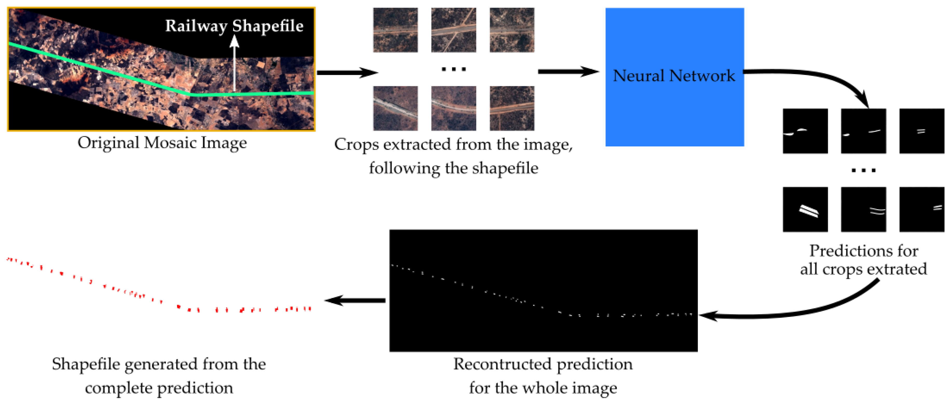
Therefore, it is fundamental to early identify and monitor erosion in railway lines in order to prevent major consequences. Typically, such identification and monitoring are performed in loco, but the accessibility to high-resolution aerial imagery has allowed for analyzing larger areas quickly and with less effort. In this case, erosion identification is conducted by specialists that must visually recognize them into huge aerial photography datasets by examining every image. It is a faster process than monitoring physically, but still a time-consuming and slow task. Thus, with the purpose of trying to speed up the process, automatic methods to perform erosion identification using remote sensing images appear as an economic and appealing alternative for the society.
Towards such an objective, during the last few decades, researchers have proposed and experimented distinct machine learning-based approaches to automatically perform erosion identification in aerial images. In all those methods, the feature extraction, responsible for quantitatively describing the images based only on its internal pixels, is a fundamental step, given that spatial feature representation in a suitable way is the key for generating good pattern classifiers. However, extracting meaningful features of erosion areas is a complicated task given the: (i) high variation in size, since an erosion can vary from few centimeters to meters in both length and depth, (ii) distinct shapes and textures, as an erosion can occur in many different patterns and places, (iii) high temporal variability, since an erosion may vary notably with the action of time, and (iv) high difference in illumination and shadows, common aspects in remote sensing images. Hence, as important as automating the process is creating a good feature representation for the remote sensing images in order to allow the machine learning approaches to capture all feasible information and, then, accurately perform erosion identification.
Focused on creating good feature representation, a prominent technique, called deep learning [
4], can learn the adaptable and specific features and the classifiers in a single training stage (end-to-end). Deep Learning is a sub-field of machine learning that primarily focuses on multi-layered neural network models. These models have, inherently, a feature learning step that allows a better data-driven encoding of feature. This process of feature learning is performed automatically by the models, thus eliminating the necessity of manually setup feature extraction algorithms. Convolutional Network (ConvNet) [
4] is the most common deep learning method for learning visual features in computer vision applications, including remote sensing ones [
5]. The success of this network for image related applications is mainly due to the fact that it exploits the natural stationary property of the images, i.e., the statistics of one part of the image are assumed to be the same as those of any other part [
6]. ConvNets are able to learn and combine features from different levels of abstraction: (i) low-level information (such as corners and edges) is captured in the first layers; (ii) intermediate layers are capable of learning mid-level patterns (as object parts); and (iii) high-level information (such as whole objects) are learned by the last layers.
Given the benefits of deep learning, the main objective of this work is to develop an effective tool (based on supervised learning) for erosion identification. Towards such goal, we introduce a new framework, based on ConvNets, to perform supervised erosion identification in railway lines using high-resolution aerial image sets. Precisely, we tackle the erosion identification as a (semantic) segmentation (also known as pixel classification) task, in which each pixel of the input is labeled into one of the classes. Although more difficult, such task allows a better definition of the erosion boundaries which can lead up to other useful information, such as the exact land area covered by the erosion, a possible estimate of the price to fix the problem, and others. All this knowledge can be used by agents to propose better plans of actions, define priorities, and so on.
In order to define the best deep learning segmentation technique to be integrated into the proposed framework,
six successful supervised approaches were evaluated in this work, including: (i) Pixelwise [
7], a segmentation algorithm that classifies each pixel independently using context windows, (ii) Fully Convolutional Network (FCN) [
8], one of the first fully convolution architectures proposed for pixel labeling, (iii) Deconvolution network [
9,
10,
11], an encoder–decoder fully convolutional architecture proposed for semantic segmentation, (iv) DeepLabV3+ [
12], a multi-scale semantic segmentation approach that combines atrous spatial pyramid pooling with an encoder–decoder architecture based on depthwise separable convolutions, (v) Dynamic Dilated ConvNet (DDCN) [
5], a pixel labeling approach based on dilated convolutions that exploits multi-scale information by allowing the training with dynamic patch sizes, and (vi) Mask R-CNN [
13], an instance segmentation technique which proposes regions and then annotates each pixel of such proposals by using a fully convolutional network.
Although the proposed framework can be used as standalone package, we encapsulate it as a plugin for the software ArcGIS (
https://www.arcgis.com/). The main advantage of using the proposed framework as an ArcGIS plugin is the possibility of combining the state-of-the-art technique (embedded into the plugin) with the already implemented visualization, manipulation, and processing tools of ArcGIS. Note that the source-codes for the framework and for the ArcGIS tool are publicly available (
https://github.com/Gabriellm2003/Deep-Learning-ArcGIS-Plugin).
In summary, we claim the following contributions for this work:
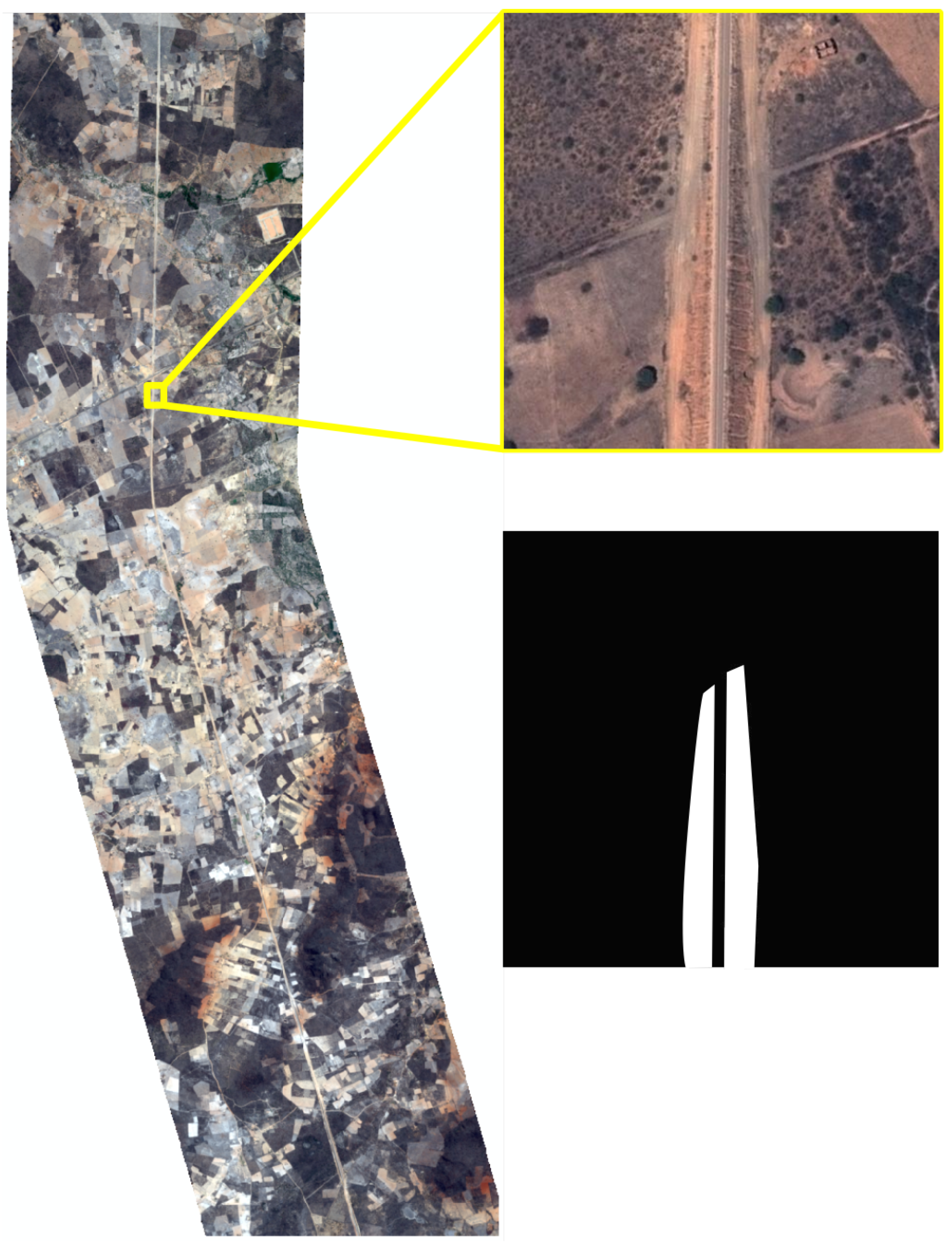
a novel Railway Erosion dataset composed of 1960 high-resolution satellite images,
an evaluation and analysis of six deep learning-based methods to perform erosion identification in an aerial high-resolution remote sensing dataset,
a new tool for erosion identification using satellite imagery,
a new plugin for the ArcGIS software based on the proposed tool.
It is important to emphasize that, as far as the authors are aware, this is the first work to use deep learning-based techniques to perform erosion identification in remote sensing images.
The remainder of this paper is structured as follows. Related works are presented in
Section 2.
Section 3 presents, in detail, all deep learning-based techniques evaluated in this work. In
Section 4, we present the framework and ArcGIS plugin. The experimental protocol for the evaluation of the methods is presented in
Section 5.
Section 6 presents the produced results while
Section 7 discusses such outcomes. Finally,
Section 8 concludes the work, pointing out the findings and future work.
2. Related Work
The increasing availability of high-resolution aerial imagery (provided by new sensor technologies) allows the deployment of a growing number of remote sensing datasets which, in turn, opens new opportunities for Earth Observation applications, such as erosion identification. However, as introduced, performing such task using manual efforts is costly and automatic methods appear as an attractive alternative. In fact, over the years, several techniques [
3,
14,
15,
16,
17,
18,
19,
20,
21,
22,
23] have been proposed to perform erosion identification using remote sensing datasets.
Benzer [
14] exploited distinct factors—including rainfall erosivity, soil erodibility, and vegetative cover—to perform erosion identification. Particularly, those factors, which consist of a set of logically related geographic features and attributes, were combined using the RUSLE model [
24] in order to finally perform the erosion identification. In [
15], the authors perform soil erosion identification and monitoring using multi-temporal and multi-resolution Digital Terrain Models (DTMs) produced from images captured by Unmanned Aerial Vehicles (UAVs). They calculated the difference between the DTMs in two different points in time to understand and monitor the gully volume change. Eltner et al. [
16] also used high precision DTM, extracted from UAV as well as from terrestrial laser scanning (TLS), to perform multi-temporal change detection of erosion areas.
More recently, Liu et al. [
3] proposed a system to perform gully erosion identification in catchments using high-resolution Digital Elevation Models (DEMs) and ortho-mosaics produced from images captured by UAV. Their approach combines an object segmentation algorithm, called Multi-resolution Image Segmentation Algorithm (MRIS) [
25], with random forest to perform erosion identification. In [
17], the authors classified different soil erosion types using terrain and spectral attributes obtained from hyperspectral images. Different machine learning algorithms—such as Support Vector Machine (SVM), random forest, and shallow Artificial Neural Network (ANN)—are trained to predict the type of soil erosion. Arif et al. [
18] used a simple Multi-Layer Perceptron (MLP) network to perform erosion classification. Such network receives as input five factors of erosion control—erosivity, erodibility, length and slope, land cover management, land conservation practice, and the spectral signature of a SPOT 5 multispectral image with four bands/channels and outputs the erosion classification. Krenz et al. [
19] exploited vegetation images and topographic information, also captured by a UAV, to identify areas of soil degradation. In [
20], authors proposed to employ different indexes—such as fractional vegetation coverage, nitrogen reflectance index, yellow leaf index, and bare soil index—to perform erosion detection. Specifically, such indexes, derived from remote sensing imagery, were integrated to create a final model through Principal Component Analysis (PCA). In [
21], the authors exploited multiple indexes, computed over MODIS data, to perform erosion assessment. Such indexes were used to train a random forest model that is responsible to perform the final erosion mapping. Gianinetto et al. [
22] proposed the dynamic version of the RUSLE model [
24]. In fact, the original formulation was altered to incorporate variations in rainfall erosivity and land-cover allowing the estimation of both spatial and temporal land-cover changes. Peponi et al. [
23] combined geographic information systems and shallow ANNs to design a model that forecasts the erosion changes using satellite images.
Our work is the first one in erosion recognition that focuses on the segmentation of erosion areas in railway lines using high-resolution aerial image sets. Furthermore, although some of the previous works [
17,
18,
23] employ artificial networks to tackle the problem, none of them use deep learning-based approaches to perform erosion segmentation. In fact, as far as we know, this is the first work to use deep learning for erosion segmentation in high-resolution remote sensing images.
3. Background
This section aims to explain all deep learning methods that were evaluated in this work for erosion identification. Such semantic segmentation approaches were selected based on their popularity and performance for different applications and images, including computer vision [
8,
9,
10,
11,
12,
13], remote sensing [
5,
7,
26,
27,
28,
29,
30], medical [
31,
32,
33,
34,
35], and so on. However, although their success in different domains, as aforementioned, those methods were never evaluated in the erosion identification task.
Section 3.1 describes the pixelwise [
7] strategy and its architecture. Fully Convolutional Network (FCN) [
8] is presented in
Section 3.2, while
Section 3.3 introduces the concept of Deconvolution Network and its architecture [
9,
10]. In
Section 3.4, the famous fully convolutional DeepLab [
36] architecture is detailed.
Section 3.6 presents the Mask R-CNN [
13] and its idea of performing object detection and segmentation at the same time. Finally,
Section 3.5 explains the Dynamic Dilated ConvNet (DDCN) concept and architecture.
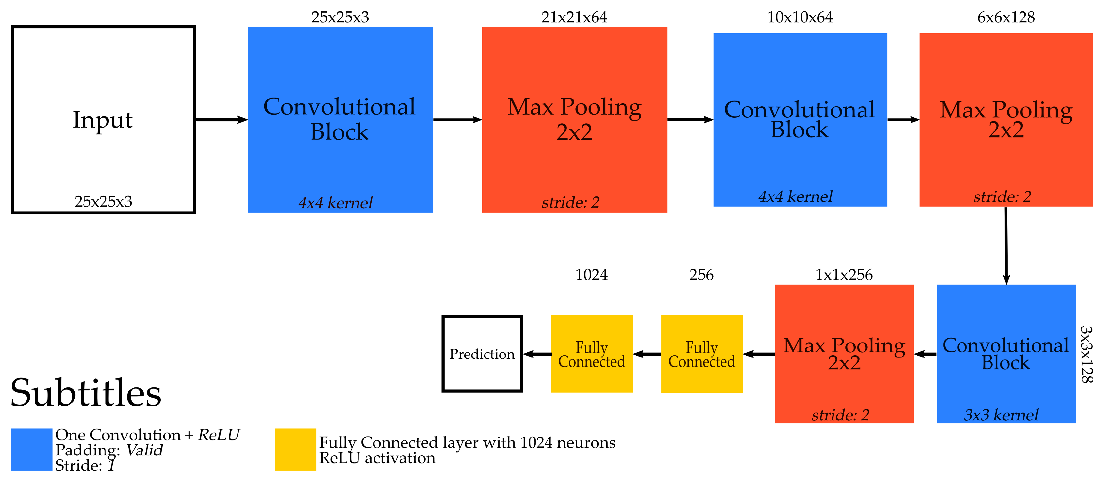
3.1. Pixelwise Network
The first deep learning-based strategy evaluated in this work is the pixelwise one [
7]. In such technique, each pixel of the input image is classified independently. Precisely, each pixel is represented by a context window, i.e., overlapping fixed-size patches, in which each one is centered on a specific pixel helping to understand the spatial patterns around that pixel. Observe that these context windows are really necessary because the pixel itself has not enough information to be used in its classification. Such patches are, in fact, used to train and evaluate the network. In both processes, the ConvNet outputs a class for each input context window, which is associated with the central pixel of the window. The main advantage of this method is the possibility of classifying each and every pixel based on its context, which creates detailed high-resolution outputs [
7]. However, the computational resources required for these techniques are huge since every pixel of the image becomes a context window for the network.
An overview of the network architecture, based on the pixelwise strategy, evaluated in this work is presented in
Figure 1. Such network, proposed by [
7], receives as input
context windows and has three convolutional and max-pooling layers, and two fully-connected ones. Furthermore, after each fully-connected layer, there is a dropout [
4] with a 50% chance of randomly dropping a neuron. It is important to emphasize that, because of its advantages [
7], Rectified Linear Unit (ReLU) [
4] was the processing units used in all layers of this ConvNet.
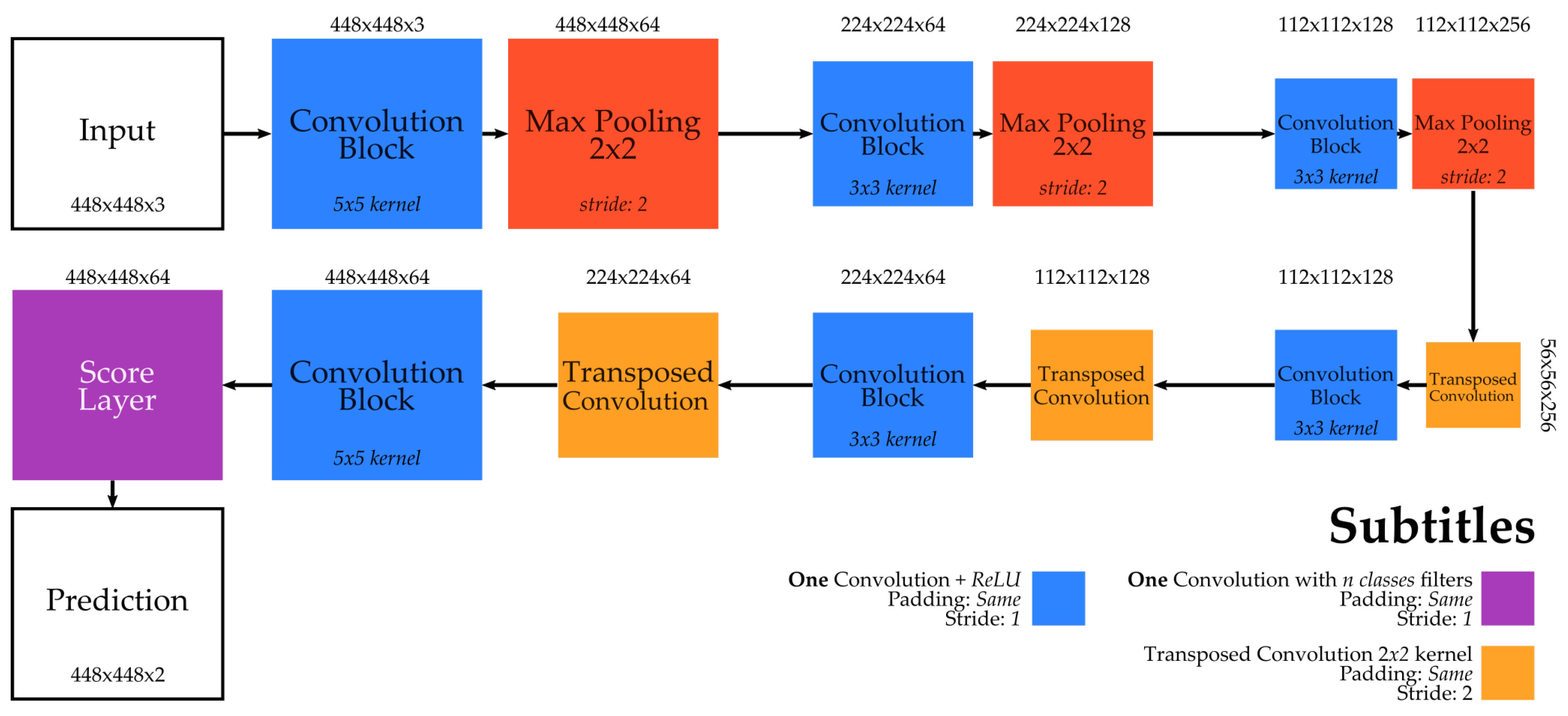
3.2. Fully Convolutional Network (FCN)
Towards a precise semantic segmentation using less computational resources, there is the Fully Convolutional Network (FCN) [
8]. Such network takes as input the original image and returns, as output, another image (i.e., the dense prediction), with the same resolution of the input, but with each pixel associated with a class. This is possible due to the use of deconvolution layers [
37] that learn how to upsample the feature maps and produce the final dense prediction.
Figure 2 presents the FCN architecture evaluated in this work. This network is very similar to standard ConvNets (such as the one proposed in the previous section) but has subtle modifications. Particularly, this FCN does not have fully-connected layers being essentially composed of convolution and max-pooling ones. This allows the network to preserve the spatiality of the feature maps (since fully-connected layers lose such property), which is required in order to perform finer dense classification. In addition, as aforementioned, this network uses deconvolution layers [
37] to upsample the prediction into pixel-dense outputs. This is essential because the convolution and max-pooling layers reduce the resolution of the input, whereas the deconvolution ones restore the spatial size outputting a prediction with the same height and width of the input image.
Aside from this, note the use of elementwise addition in this architecture. This is explored because creating the final prediction map using only the classification performed by the last convolution may result in deceptive prediction maps [
8]. Thus, to overcome this problem, skip connections were incorporated into the architecture (usually coming from pooling layers). These connections allow the network to combine (via elementwise addition) prediction maps (created from distinct feature maps) that combine information from fine (final) and coarse (initial) layers, allowing the model to make local predictions that respect the global image structure.
The obvious advantage of this method is a reduced computational complexity, given that it classifies patches instead of pixels. Furthermore, the prediction maps can have distinct resolution for training and testing, i.e., the size of the training images can be different from the testing ones which gives more independence for the ConvNet. Although using one deconvolutional layer to upsample the output of a ConvNet provides dense outputs, the result may be imprecise because the upsampling process performed is too simple. Thus, usually more than one upsample operation is used, as in the case of the evaluated architecture. Even though this model uses two deconvolutions, the direct upsample to the output forces the last layer to learn the transformation from a smaller space to a larger, at the same time that is directed influenced by the prediction. This can create undesirable results once the layer has to focus in two different tasks.
3.3. Deconvolution Network
Deconvolutional networks [
9,
10,
11] try to overcome the aforementioned issue by using multiple deconvolutional layers [
37] to produce the final dense prediction (from a coarse feature map) with the same resolution of the input image. Normally, such networks are based on encoder–decoder architecture. The encoder works as a fully ConvNet (without the final classification layer) by running the following pipeline: it receives input images; learns the visual features by using standard convolution and max-pooling layers; and outputs a coarse feature map. The decoder receives a coarse map generated by the encoder as input. It learns to upsample these features by using deconvolution layers to increase the spatial resolution of the coarse map gradually. The decoder output is a prediction map with the same dimensions (h × w) of the original input image. The encoder–decoder functions as one larger model. That is, they are trained together in an end-to-end manner by using classical feedforward and backpropagation algorithms, and are also in used/tested in a connected fashion.
Figure 3 presents the deconvolutional network architecture exploited in this work. The encoder part of this network is composed of three convolution layers (each one followed by a max-pooling). It receives the input image and outputs a
coarse feature map. The decoder part has three deconvolution layers (each one followed by a convolution layer), very similar to [
11,
12]. This part receives the coarse feature map (produced by the encoder) and outputs the final prediction image.
The biggest advantage of this technique relies on the use of more than one deconvolution layer. It gradually improves the spatial information of the outcome resulting in smoother predictions than the fully convolutional networks [
8]. On the other hand, the disadvantage of such approach is the training load. Since the network is significantly larger, the optimization may be slow and difficult due to the huge number of trainable parameters.
3.4. DeepLabV3+
Recently, researchers [
5,
12,
38,
39,
40,
41] noticed that smoother predictions could be generated if the input image resolution was not reduced substantially, i.e., if the input information was preserved over the layers. However, this comes with a problem: by preserving data resolution, the networks would not be able to exploit certain benefits that they are capable of when downsampling the data, such as the increase of the receptive field (and, consequently, of the observable area) [
4]. To overcome such a problem, dilated convolutions [
42] were proposed. Such layers are capable of increasing the receptive field whereas preserving the resolution, i.e., no downsampling in the data are performed.
Over the years, several methods have been proposed to exploit the advantages of dilated convolutions [
5,
12,
38,
39,
40,
41]. Among such approaches, one of the first (and most famous) techniques proposed for semantic segmentation is the DeepLab [
12,
38,
40,
41]. This method, based on fully convolution networks, has several version (V1 [
38], V2 [
40], V3 [
41], and V3+ [
12]) that exploits the same concept: the input resolution is downsampled in the first layers from which it is kept constant by the final dilated convolutions. Essentially, the differences between the versions are the use of more dilated convolutions to make the method more robust.
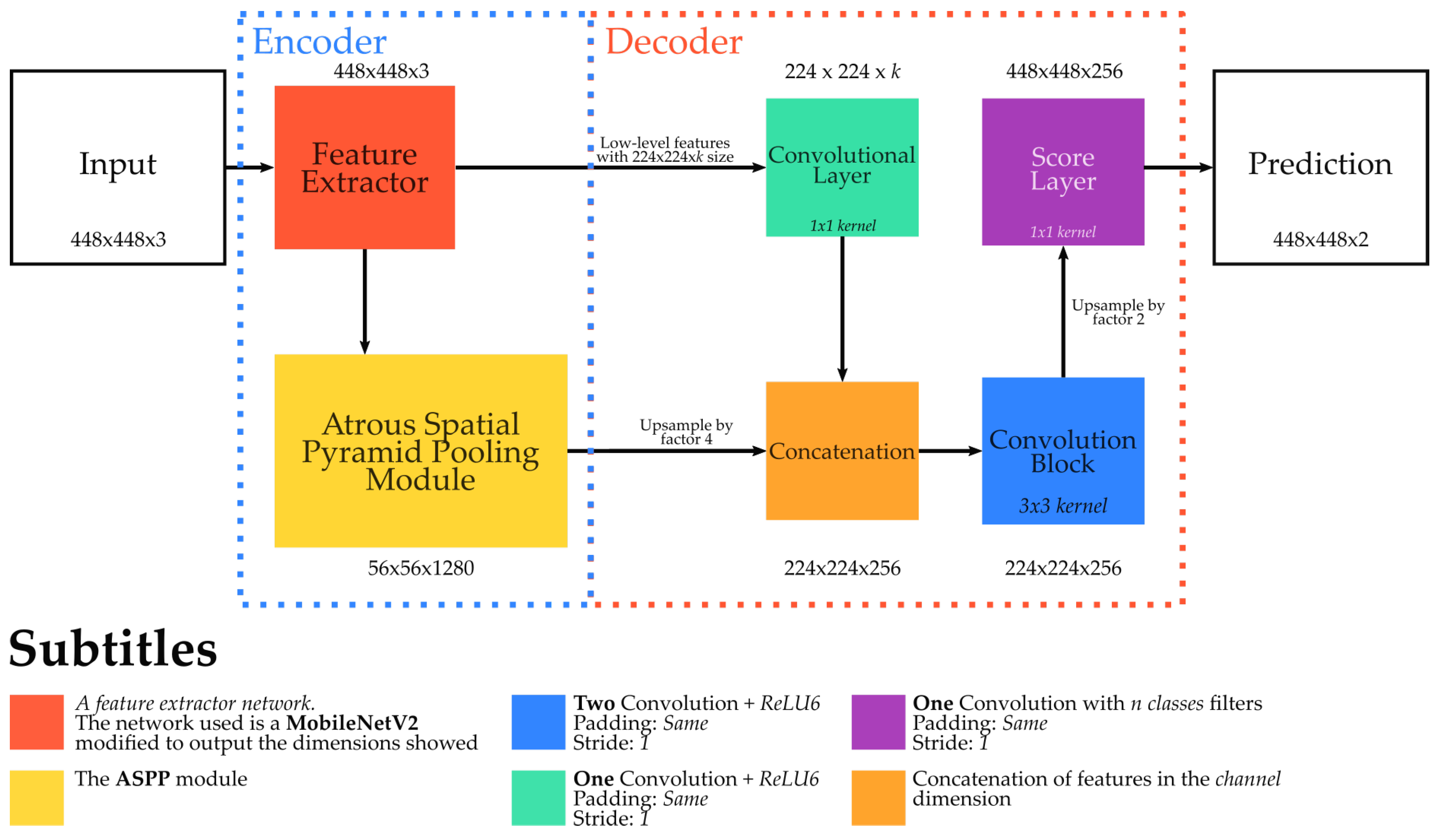
In this work, we evaluated the DeepLabV3+ version [
12], whose architecture is presented in
Figure 4. Technically, such network can be seen as an encoder–decoder architecture.
In the encoder part, it first uses a (usually pre-trained) network to extract low-level features. Different networks can be used as a backbone to extract the features, such as Xception [
43] and MobileNetV2 [
36]. In this work, we use a
pre-trained (on VOC Pascal dataset [
44])
MobileNetV2 network [
36], in which 1280
feature maps are extracted from the layer just before the classification one. Such features are further processed, in the encoder part, by an Atrous Spatial Pyramid Pooling (ASPP) module. This component is composed of a set of atrous convolution layers [
42] that process the same input features but with different dilation rates, allowing it to capture and aggregate multi-scale information.
The decoder part concatenates the low-level features (extracted by the Feature Extractor module) with (a bilinear upsampled version of) the multi-scale features extracted by the ASPP module. Then, it further processes the concatenated features using standard convolution layers. Finally, a simple bilinear upsampling is performed to retrieve feature maps with the same resolution of the input data that are then, processed using a convolution layer, producing the final prediction map.
An advantage of the DeepLabV3+ network [
12] is its capacity of generating a high-quality segmentation mask, which is achieved by not reducing the initial resolution substantially. The disadvantage would be that the input data are still downsampled, in the first layers of the backbone network, resulting in a likely loss of valuable information.
3.5. Dynamic Dilated ConvNet
To try to overcome previous drawback, a recent method, called Dynamic Dilated ConvNet (DDCN) [
5], takes the concept of preserving the input image resolution to the extreme. Specifically, this semantic segmentation technique proposes a new multi-scale training strategy that employs dynamic input sizes to converge a fully dilated convolution network that never reduces the input image.
The method receives as input the images and distributions over the possible sizes that the network input image (i.e, patch) may have. In this work, we used a uniform distribution that allows the method to select an input size from three possibilities: , , and . In each iteration of the training, an input size is randomly selected from the given distribution and a new batch composed of distinct images (when compared to other batches) of the pre-selected input resolution is created and used to converge the model. It is important to note that the multi-scale information is learned during the model training by composite batches of inputs with multiple sizes. In the prediction phase, the algorithm selects, based on scores accumulated during the training for each evaluated input size, the best resolution for a given problem. The technique processes the testing images using batches composed of images with the best-evaluated resolution.
Several different architectures could be used with this training strategy, such as fully convolution [
8,
12,
38,
40,
41] and deconvolution networks [
9,
10,
11]. Although these networks may be able to process inputs of varying sizes, they may have problems related to a possible high variation of the input size. Precisely, such networks require the input to be large enough so that they can downsample it to generate a coarse map, which is then upsampled to the original input size. The network may not be able to generate this coarse map if the input is too small.
To overcome this problem, the authors in [
5] proposed a new network composed uniquely of dilated convolutions [
42] that never reduces the input image. This fully dilated network fits perfectly into the proposed multi-scale training strategy as it is capable of processing inputs of any size (without constraints since no downsampling would be performed at all) while still outputting results with the same resolution of the input data. Note that, unlike DeepLabV3+ [
12], this network never reduces the input image, preserving its resolution from end-to-end, allowing the model to extract more useful information and, consequently, it can produce smoother predictions.
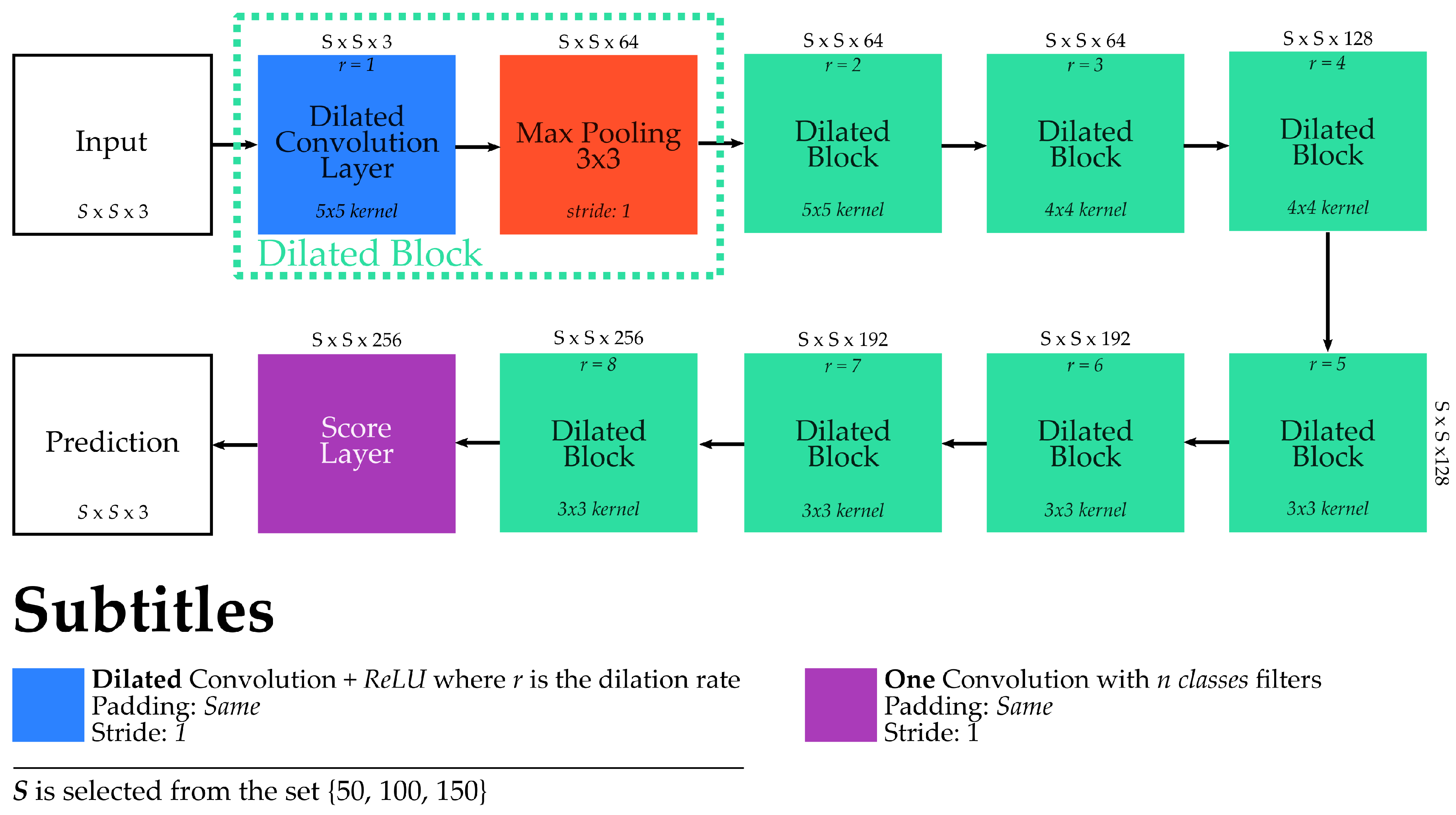
The fully dilated network architecture evaluated in this work is presented in
Figure 5. It has eight dilated blocks, each one composed of a dilated convolution and a max-pooling layer. Besides that, it is worth mentioning that the pooling layers do not downsample the input given with a specific configuration of stride and padding (i.e., stride 1 and padding same).
Specifically, the dilated convolutions of first two blocks have filters with dilation rates 1 and 2, respectively. The convolution layers of the following two dilated blocks have kernel filters but rates 3 and 4, correspondingly. The last four dilated blacks have convolution layers with smaller filters () but higher dilation rates (5, 6, 7 and 8, respectively). Finally, after all those layers, there is a final convolution layer responsible for generating the final dense predictions.
Looking at pros and cons, an advantage of the DDCN [
5] is the possibility of exploiting multi-scale information without increasing the complexity of the network while preserving the initial image resolution, which can help the network to learn even more representative patterns from the data. The main disadvantage of this approach is the training time. Since the input image is not downsampled, the model needs more time to converge as the processing time of each layer is proportional to the input data resolution [
45].
3.6. Mask R-CNN
Even more recently, new approaches for performing object identification were conceived based on the concept of instance segmentation. Differently from semantic segmentation techniques (such as the previous ones presented in this Section), which output dense predictions inferring a class for every pixel of the input image, instance segmentation techniques try to first identify and locate the object instance (delineating its boundaries), and after that they segment the object of interest. Therefore, the final prediction of instance segmentation approaches may not be totally dense, i.e., only the interested objects will be identified and segmented in the final outcome, leaving all the uninterested parts of the input image without a label classification.
In this work, we evaluated the Mask R-CNN [
13], an instance segmentation technique that detects and segment pixels of the object instances by using a Fully Convolutional Network. Technically, the Mask R-CNN [
13] is strongly based on the Faster R-CNN [
46], an object detection approach that receives input images, detects the object instances, and outputs the bounding boxes proposals for object detection. The Mask R-CNN technique [
13] uses the Faster R-CNN [
46] to first generate the object instance bounding boxes and then segments such proposals to produce the final prediction map for each object instance. Overall, the Mask R-CNN [
13] efficiently detects object instances in an image and simultaneously generates a high-quality thematic map for each detection by adding just a small computational overhead to the Faster R-CNN [
46].
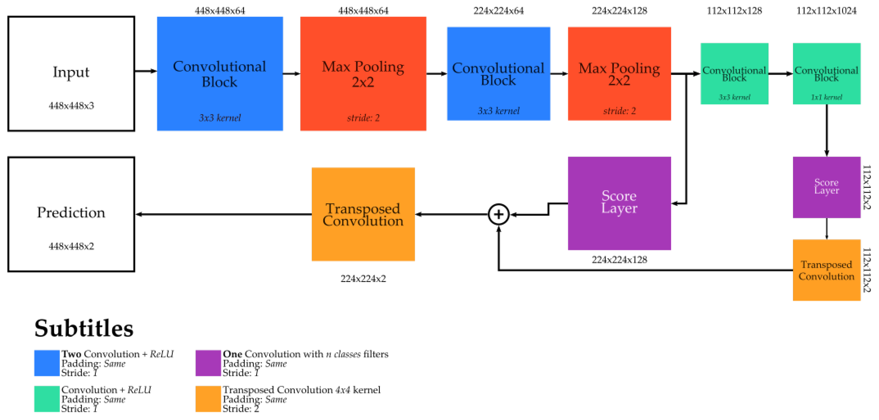
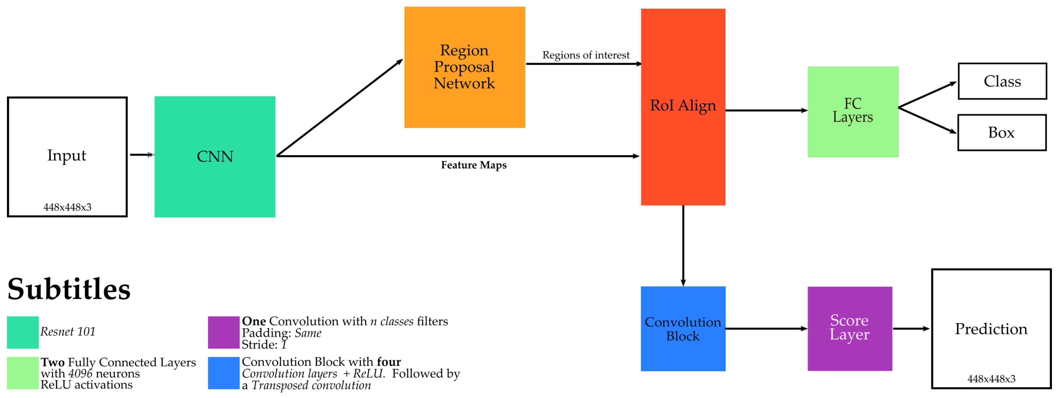
An overview of the Mask R-CNN architecture [
13] is presented in
Figure 6. The first module of this architecture, called here CNN, is responsible to extract the features and create a representation for the input images. In this work, this module is actually composed of a
ResNet-101 [
47],
pre-trained on the ImageNet dataset [
48]. Then, a module, called
Region Proposal Network (RPN), is responsible to create bounding proposals, while the module
Region of Interest (RoI)
align performs the alignment between the feature maps (extracted by the CNN module) with the proposals. Then, the network architecture divides into two branches. The first one, composed of the
Fully Connected (FC)
Layers, is responsible to detect and classify the proposals while the second one, composed of
Convolution Block and
Score Layer, classifies the pixels of the proposals, segmenting the objects. Note that, except for the second branch of the last part, all other modules are part of the original Faster R-CNN architecture [
46].
An advantage of the Mask R-CNN [
13] (when compared to other methods) is its capacity of generating high-quality segmentation mask for each object, since it classifies each instance separately. On the other hand, one disadvantage of this approach may be the training. Even using a pre-trained network in the CNN module, Mask R-CNN [
13] has several other modules (each with lots of parameters) that needed to be trained. Therefore, the training of this technique may not be that easy.
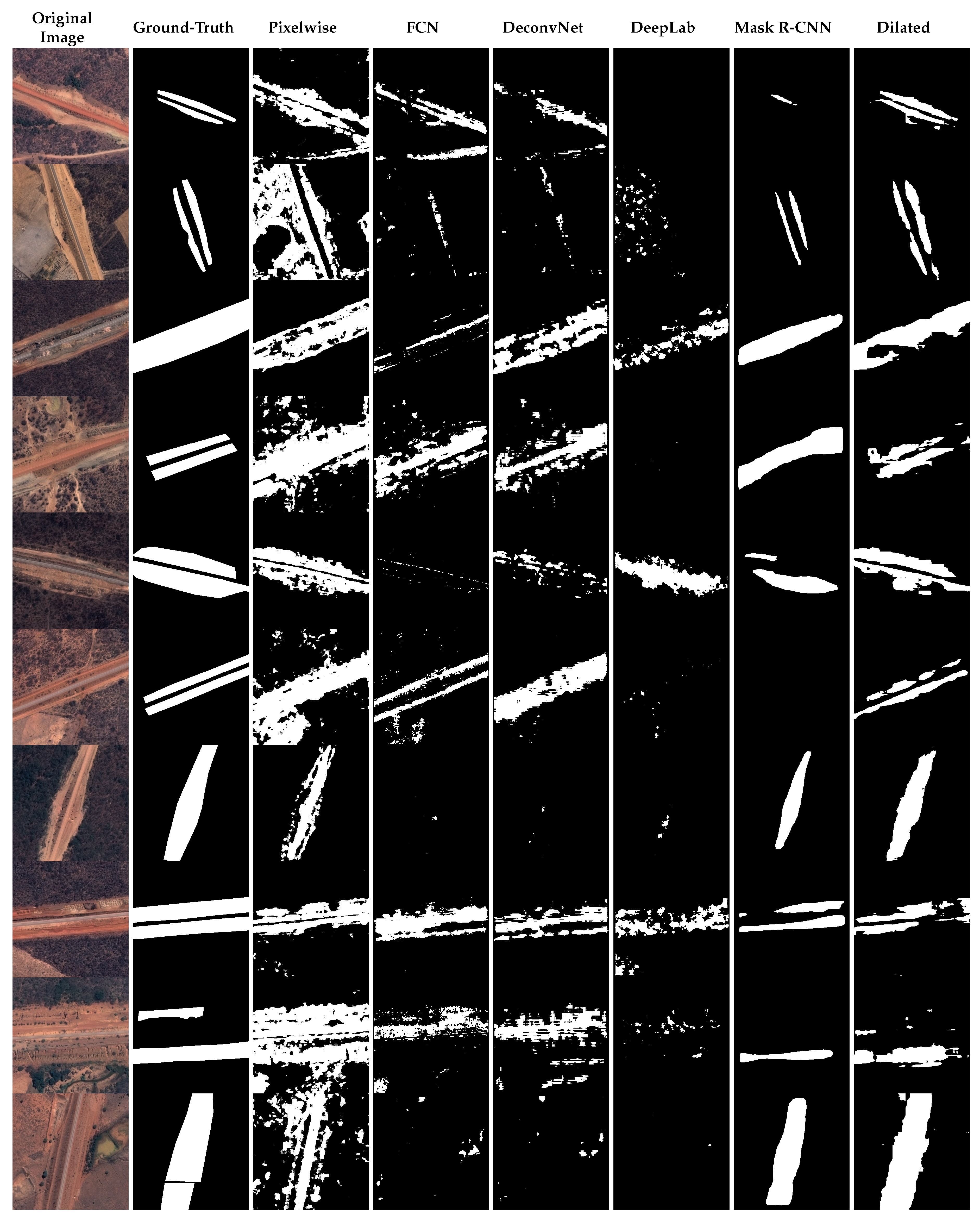
6. Results
A systematic set of experiments was conducted to: (i) evaluate the effectiveness and robustness of the aforementioned approaches, and (ii) define the best technique to be integrated into the proposed framework and plugin.
The obtained results of the evaluated methods are presented in
Figure 11. Moreover,
Table 2 relates the obtained results with the training time (in hours per fold) for each evaluated technique. In addition, a visual comparison of the outcomes generated by each approach is presented in
Figure 12.
Overall, all tested methods, except the Dynamic Dilated ConvNet [
5], produced very similar results for all evaluated metrics while having a comparable training time. The DDCN [
5] also yielded similar results, in terms of normalized accuracy, when compared to all other methods, as seen in
Table 2. However, considering the other metrics, it is possible to note that the DDCN [
5] achieved the best results outperforming all other techniques that had very similar performance as previously stated, as seen in
Figure 11.
The explanation for this outcome is two-fold. The first one would be due to the training strategy, employed by the Dynamic Dilated ConvNet [
5] that allows the model to easily aggregate multi-scale information. The second one would be that such dilated network never downsamples the input image, preserving its resolution during all processing. This allows the network to extract even more useful information from the data. The drawback of this method is training time (as can be seen in
Table 2), which is huge compared to the other evaluated methods. Again, this may be justified by the fact that the input image is not downsampled, resulting in a model that requires more time to converge as the processing time of each layer is proportional to the input data resolution [
45].
In addition to the previous results,
Figure 12 presents several visual outcomes generated by all experimented approaches. As expected, the best visual outcomes are produced by the DDCN [
5]. Again, this may be explained by the dynamic multi-scale training strategy (employed in this technique) and the preservation of the input resolution through the network. Hence, despite the disadvantages and based on (both quantitative and qualitative) obtained results, the Dynamic Dilated ConvNet [
5] was the technique selected, implemented, and encapsulated into the aforementioned ArcGIS plugin.
7. Discussion
As presented in the previous section, the DDCN [
5] technique yielded the best outcomes and was integrated into the final version of the proposed tool and ArcGIS plugin. However, as aforementioned, the main disadvantage of such an approach is its demanding training time. Although this might seem to be a problem, note that the computational time of this technique is expensive only during the training phase. The inference (or testing) time of this method is small since no optimization is carried out in the model anymore [
4], i.e., no back-propagation calculations are computed and only the feed-forward step is performed. Therefore, once the model is trained, it can be used repeatedly to identify erosion areas in different scenarios without consuming too much time.
Considering the compulsory computation time of the inference procedure, we argue that the proposed framework is useful and can be used to decrease both the time and resources required to perform erosion identification. Comparing to the current approaches, such as the
in loco monitoring and the manual process, the inference time and training cost is negligible. This is because
in loco monitoring requires at least one specialist to visit each investigated location to assess the erosion level while the manual investigation requires specialists to visually analyze large-scale remote sensing datasets in order to recognize erosion areas in different scenarios and cases. Since both situations require at least one specialist to manually identify erosion areas, the actual computational cost of training and using a Dynamic Dilated ConvNet [
5] model outweighs the time and economic cost involved in those situations.
Another important aspect to mention is that, in this work, an ArcGIS plugin that encapsulates the proposed framework, was implemented, opening opportunities for a simplified use of this powerful deep learning-based technique by non-programmers and users. In fact, we expect that any end-user, with minimal knowledge of the ArcGIS software and no programming skills, is able to exploit this plugin and speed up their work.
Overall, we believe that the solution and plugin proposed in this work may help several distinct public and private organizations. An example of usefulness of this work would be to assist control agencies in auditing public works. These auditing process is, usually, realized through
in loco monitoring, or visual analysis of remote sensing imagery, performed by agents [
52,
53]. In cases like this, automatic machine learning-based methods can be used as an acceptable solution to speed up the audit process.
Aside from this, note that no comparison with baselines from the literature was performed. This is because, although there are several works performing erosion identification [
3,
14,
15,
16,
17,
18,
19,
20,
21,
22,
23], most of them are based on the combination of multiple information (such as Digital Terrain Models [
15], Digital Elevation Models [
3], and temporal information [
16,
22,
23]). Due to this, such existing approaches can be seen as different from the proposed tool, which is exclusively based on remote sensing images. Therefore, given this essential difference, we argue that a comparison between those works from the literature and the proposed one would not be totally fair.
8. Conclusions
In this paper, we proposed a novel framework, based on Convolutional Networks, to perform erosion identification (i.e., segmentation and classification) in railway lines using high-resolution aerial image sets. In order to define the best deep learning-based approach to be integrated into the proposed framework, we evaluated, using a proposed Railway Erosion dataset,
six existing techniques, including: (i) Pixelwise [
7], (ii) Fully Convolutional Network (FCN) [
8], (iii) Deconvolution network [
9,
10,
11], (iv) DeepLabV3+ [
12], (v) DDCN [
5], and (vi) Mask R-CNN [
13].
Experiments made on this dataset have shown that the Dynamic Dilated ConvNet [
5] produces the best results (in terms of IoU and Kappa) for the proposed dataset. Based on obtained results, the DDCN [
5] was the technique selected and implemented in proposed framework, which was then converted to a new plugin for the software ArcGIS.
The presented work opens opportunities towards a simplified use of deep learning methods for better identification of erosion in railway lines, an important application to solve potentially impactful problems, such as economic losses and human causalities. Furthermore, we argue that the proposed framework (and plugin) is able to significantly decrease the time invested in identifying erosion in large areas, such as the Transnordestina Railway. Even if the model’s training time is substantial, the inference time is small and the effort required to analyze and identify erosion areas in the proposed dataset is still smaller than an in loco monitoring or a manual observation of the images.
As future work, we plan to increase the proposed dataset by including images from railway lines of other parts of the world, making it more robust and representative. We also intend to experiment and integrate more deep learning-based algorithms into the proposed tool and plugin. Finally, we also plan to evaluate unsupervised deep learning methods for erosion identification, comparing such approaches with supervised ones.

 ,
, 


