Abstract
Similar to light detection and ranging (lidar), profile radar can detect forest vertical structure directly. Recently, the first Ku-band profile radar system designed for forest applications, called Tomoradar, has been developed and evaluated in boreal forest. However, the physical relationships between the waveform and forest structure parameters such as height, leaf area index (LAI), and aboveground biomass are still unclear, which limits later forestry applications. Therefore, it is necessary to develop a theoretical model to simulate the relationship and interpret the mechanism behind. In this study, we extend the Radiosity Applicable to Porous IndiviDual objects (RAPID2) model to simulate the profile radar waveform of forest stands. The basic assumption is that the scattering functions of major components within forest canopy are similar between profile radar and the side-looking radar implemented in RAPID2, except several modifications. These modifications of RAPID2 mainly include: (a) changing the observation angle from side-looking to nadir-looking; (b) enhancing the ground specular scattering in normal direction using Fresnel coefficient; (c) increasing the timing resolution and recording waveform. The simulated waveforms were evaluated using two plots of Tomoradar waveforms at co- and cross- polarizations, which are collected in thin and dense forest stands respectively. There is a good agreement (R2 ≥ 0.80) between the model results and experimental waveforms in HH and HV polarization modes and two forest scenes. After validation, the extended RAPID2 model was used to explore the sensitivity of the stem density, single tree LAI, crown shape, and twig density on the penetration depth in the Ku-band. Results indicate that the backscattering of the profile radar penetrates deeper than previous studies of synthetic aperture radar (SAR), and the penetration depth tends to be several meters in Ku-band. With the increasing of the needle and twig density in the microwave propagation path, the penetration depth decreases gradually. It is worth noting that variation of stem density seems to have the least effect on the penetration depth, when there is no overlapping between the single tree crowns.
1. Introduction
There are two major active remote sensing technologies, light detection and ranging (lidar) and radio detection and ranging (radar). Lidar uses optical wavelengths, while radar transmits microwave radiation and records echoes from the target objects. In forestry inventories and monitoring programs, lidar (such as ICEsat or GEDI) can only collect sparse measurements for large areas, but radar has the advantage of continuous measurements over large areas. Theoretically, given a radar sensor with a fixed wavelength, an incident angle, and a polarization mode, the penetration depth and the backscattering intensity or interference should be correlated to target properties (e.g., soil roughness, moisture, or forest biomass). Thus, radar technology, primarily synthetic aperture radar (SAR), is capable of mapping large-scale forest biomass over the past three decades [1,2,3,4].
1.1. Microwave Methods for Forest Vertical Structure Retrieval
The forest vertical structure is not easy to retrieve from SAR images. For this purpose, tomography technique, an extension of multi-baseline interferometric, has been proposed to obtain the vertical distribution of backscattering energy in forest. Several studies have achieved the acquisition of forest height, aboveground biomass, and forest structure dynamic changes using SAR tomography at L-band and P-band [5,6,7,8]. However, due to the difficulty in obtaining data with ideal baseline configurations, and the large uncertainty of the reconstructed energy profiles with different inversion algorithms, SAR tomography for forest structures has not yet entered operational stages. Thus, it will be interesting to develop some waveform radar sensors using microwave wavelength, called profile radar, as a complement to SAR and lidar. From 1988 to 1991, an air-borne profile radar system (HUTSCAT) was constructed, operating in X band and C band. HUTSCAT did response from boreal forest, showing clearly the contribution of forest structure and ground [9,10]. From 2012 to 2016, a lightweight Ku-band profile radar (Tomoradar), viable for unmanned aerial vehicle, was designed by the Finnish Geospatial Research Institute (FGI) [11]. Tomoradar is a Frequency Modulated Continuous Wave (FM-CW) ranging radar system with a Global Navigation Satellite System (GNSS) and Inertial Measurement Unit (IMU) system, which offer centimeter accuracy of fly trajectory information. Tomoradar on a helicopter platform can collect, continuously, full polarization backscatter waveforms within a several-meters footprint. Several works have been carried out to quantify the energy of backscatter signals from the ground and canopy, and estimate the elevations at ground level and tree top level [11,12,13,14]. For instance, Chen et al. have proven that the Tomoradar can collect the profile information clearly from tree canopy top to ground level for both co- and cross-polarizations [11]. Feng et al. have used Tomoradar to estimate ground elevation and canopy top elevation, and the root mean square errors (RMSEs) were less than 1 m, compared with lidar measurements [13]. However, until now, there are still very few radiative transfer (RT) models to explain and exploit the profile radar waveform, which limits its value.
1.2. Related Studies on Profile Radar
Hence, it is essential for a theoretical model to simulate the profile radar waveform of forests, which would support researchers for comprehensively exploring the profile radar response from forests, and probably come up with more accurate methods to forest resource mapping. The water cloud model is one of the most classical microwave scattering models, in which the vegetation is represented by a homogeneous droplet cloud [15]. By describing the vegetation as a single homogeneous layer, Karam and Fung used finite-length cylinders to establish a scattering model for defoliated vegetation [16]. Thus, it is not applicable for canopies with vertical structures. In 1990, Ulaby et al. established the Michigan Microwave Canopy Scattering model (MIMICS), which divided forest canopies into three layers: crown, trunk, and understory [17]. Another multi-layer model, MIT/CESBIO backscatter model, was proposed by Hsu et al. in 1994 to simulate the backscattering in P band, which was a first order RT model [18]. With the coupling of the MIT/CESBIO backscatter model to the architectural tree growth model (AMAP), respectively, Floury et al. simulated the Spaceborne Imaging Radar- C/X-band Synthetic Aperture Radar (SIR-C/X-SAR) data and Martinez et al. developed the HUTSCAT profile waveforms [19,20]. In 2004, Picard et al. simulated the HUTSCAT waveforms by a three-dimension (3D) RT model [21]. However, there is no study to simulate the Ku-band profile radar where the multiple scattering may not be neglected.
Recently, a three-dimension RT model, named Radiosity Applicable to Porous IndiviDual objects (RAPID version 2), was proposed, which invented a new approach to solve the radar scattering [22]. To the best of our knowledge, RAPID2 is the first shared unified model that can simulate the full spectrum radiation from optical to microwave wavelength domains, contributing to theoretical study of multi-sources data inversion. However, the initial simulation objective in the RAPID2 model is the backscattering of SAR, a side-looking radar, which cannot obtain the microwave energy profile in forests.
1.3. Aims and Objectives
The aim of this work is to simulate the profile radar waveform of forests by extending the RAPID2 model. The RAPID2 model exhibits great potential for improving the understanding of microwave response from forests and contributing to the development of multi-sensor and data fusion. Through the further extension of profile radar waveform simulation function, the advantages of profile radar, which shows the contribution of forest structure and ground more clearly, can be used to better understand the interaction. Moreover, by combining the extended RAPID2 model and forest growth model, the application of profile radar can be more extensive in the forest parameters extraction as well. For many applications using profile radar, the penetration depth tends to be a key information. Therefore, we extended the RAPID2 model to simulate the profile radar waveform of forests and analyzed the sensitivity of the signal penetration depth in various forest scenes in this research.
2. General Strategy and Framework
Focusing on the research objective, this paper is divided into three major parts (Figure 1): model extension of RAPID2, validation, and sensitivity analysis on penetration depth.
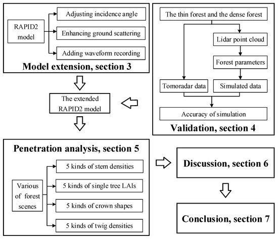
Figure 1.
The general framework of this paper.
First, we realized the RAPID2 model extension of the profile radar waveform simulation function. The extensions of the RAPID2 model are mainly on incidence angle, ground scattering, and waveform recording. As for profile radar, the incident direction is nadir-looking, instead of side-looking; thus, the transmitting and receiving directions of microwave were adjusted to be perpendicular in the extended RAPID2 model. The specular scattering of ground surface was adopted to fit the nadir incidence. Besides, the timing resolution was greatly increased to support waveform recording.
Second, to validate the simulation results of the extended model, two plots of waveform data for different forest densities, acquired by Tomoradar HH and HV polarization in October 2016, were adopted as references. The two plots are continuous, which have the similar parameters of branch/twig and dielectric constant properties, making two plots comparable. To obtain the better consistency, the 3D scenes of the two plots were built with parameters extracted from airborne lidar point cloud, which collected simultaneously with Tomoradar. Moreover, the accuracies of profile radar waveform simulations in both co- and cross- polarization for thin and dense forests were estimated.
Third, the Ku-band penetration depth at nadir incidence of various forest scenes was studied.
Accordingly, the rest of this paper is organized as follows. The RAPID model and extension are introduced in Section 3. Then, the model validation is presented in Section 4. Moreover, Section 5 illustrates the sensitivity analysis of penetration depth. In addition, Section 6 expounds the discussion of the results in detail. Finally, the conclusions are drawn in Section 7.
3. RAPID Model and Extension
RAPID model is a 3D RT model by inventing the concept of porous individual thin objects, which was proposed in 2013 (v1) by Huang et al. [23] and developed to simulate microwave backscattering in 2018 (v2) [22]. The RAPID2 model can simulate optical, lidar waveform and point cloud, thermal radiation, as well as SAR backscattering signals with unified 3D scene and input parameters. However, the vertical distribution of microwave energy in forests has not been implemented with the RAPID2 model. Thus, we extended the RAPID2 model to simulate profile radar waveform by combining the features of lidar waveform and SAR imaging modules.
In this section, the 3D scene generation and the radiosity framework in RAPID2 model is introduced in Section 3.1. Then, the extension of the RAPID2 model is described in Section 3.2.
3.1. RAPID2
RAPID2 model mainly consists of the built-in 3D scene graphical user interface (GUI) and the radiosity framework. Users can generate forest scenes by setting forest and terrain parameters. Based on the forest scene, remote sensing data of various wavelength ranges from visible/near infrared to thermal infrared and microwave are simulated using a unified radiosity model. The RAPID2 model is freely distributed online (http://www.3dforest.cn/en_rapid.html). Since the purpose of this paper is to simulate profile radar waveform, the microwave backscattering simulation of the RAPID2 model is described in the following sections.
3.1.1. Three-Dimension Scene Generation
The size and the digital elevation model (DEM) of 3D scenes could be set firstly, according to plot conditions. After that, the 3D objects, such as trees, crops, water bodies, and buildings, could be defined in the scene. In this study, trees and shrubs are the objects on ground, where the default parameters (such as height, length, width, and LAI of crown) are modified according to lidar point cloud (see details in Section 3.2).
For vegetation, the solid stem and porous crown layers generally contribute a single plant. Each porous crown layer is composed of leaves (or needles) and branches, characterized by length, thickness, orientation and density, length, and diameter, respectively. Thin discs represent broad leaves; cylinders represent needles and branches. The branches are divided into large branches and small twigs. The leaf angle distribution (LAD) and branch orientation distribution (BOD) are set from 0°to 85°with a step of 5°, assumed to be independent of azimuth. In addition, the porous objects are projected dynamically and drawn as numerous sub-leaves in the optical region or particles in the microwave region, based on the LAI, LAD, and leaf size of the crown, so as to only view factors between porous objects (not between hundreds of small particles) need to be calculated and stored. Therefore, the RAPID2 significantly reduces the huge memory requirements of large and realistic vegetation scenes and the long calculation time of view factors. For ground surface, soil facets are characterized by roughness size and correlation length. A sample forest scene in RAPID2 is illustrated in Figure 2.
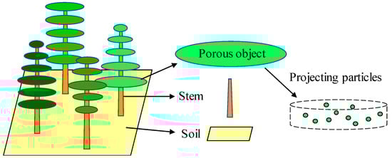
Figure 2.
A sample forest scene in Radiosity Applicable to Porous IndiviDual objects (RAPID2); the forest scene consists of porous crowns, solid stems, and soil; the porous crowns are composed of many thin layers, which would be projected as particles dynamically in microwave domain at runtime.
In microwave domain, dielectric constants of objects are of great significance for their scattering and extinction characteristics. The relative dielectric constants of stem (), branch (), leaf (), and soil () need to be pre-defined with environment temperature and moisture content [17].
3.1.2. Radiosity Framework
Comparing to classical radiosity transfer equation, the radiosity is replaced by the Stokes vector and the reflectance is replaced by the scattering matrix in RAPID2. As a result, the extended radiosity theory is able to simulate microwave scattering in RAPID2. For specular scattering, as an example, the Stokes vector () at the direction () can be expressed as:
where is the single scattering Stokes vector of object i; or is the normal direction of object j or k to object i; or is the directional view factor between j (or k) and i from or to ; or is directional scattering or transmittance matrices, and can be expressed as Mueller matrix (M):
where is the complex scattering matrix.
The scattering of a porous object is composed of Lambertian and non-Lambertian parts. The non-Lambertian part means its scattering is direction-dependent, which includes forward and specular scattering. For solid objects, such as soil and trunk, the forward scattering is minor and ignored.
The total scattering process of a forest canopy is separated into single scattering, double bouncing scattering, and multiple scattering, based on three pre-hypotheses:
- (1)
- The specular scattering is independent from Lambertian scattering.
- (2)
- The major double bouncing scatterings include the specular scattering between trunk and soil, and the specular scattering between crown layers and soil.
- (3)
- Multiple scattering only occurs from the Lambertian scattering among the porous objects.
Finally, the radar backscattering of vegetation is as follows:
The major output results of RAPID2 are the total backscattering coefficient of the scene, the backscattering coefficients of each component (crown, trunk, soil) and the simulated radar images of the scene in full polarization modes.
3.2. RAPID2 Model Extension
Table 1 presents the differences and requirements to extend RAPID2 from SAR mode to profile radar mode. Firstly, there are significantly different observation modes between SAR and profile radar, where the transmitting and receiving directions of microwave were adjusted to be perpendicular. Secondly, compared with the mixture of ground surface scattering and vegetation scattering in SAR data, the ground surface scattering is more independent and stronger in profile radar scattering. The major scattering type contributing to the ground surface scattering changes from Lambertian scattering to specular scattering in profile radar observation. Thirdly, the outputs of SAR and profile radar are different. The output of SAR includes an image and total backscattering coefficients, while that of profile radar is waveform. In consequence, the output function with high resolution of the vertical backscattering intensity records should be added to the extend RAPID2 model.

Table 1.
The difference between synthetic aperture radar (SAR) and profile radar and the extension requirements
Figure 3 further demonstrates the difference of the major ground surface scattering type between SAR and profile radar.
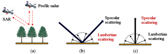
Figure 3.
The illustration of the major ground surface scattering type of SAR and profile radar: (a) observation direction of SAR and profile radar; (b) Lambertian scattering is the major ground surface scattering type in SAR data; (c) specular scattering is the major ground surface scattering type in profile radar data.
As specular scattering is identified as the main type of ground surface scattering, the intensity of the specular scattering needs to be estimated. In this paper, we adopted Fresnel scattering coefficient to acquire the co-polarization intensity of specular scattering. The co-polarization backscattering coefficient can be defined as [24]:
where the and are the Fresnel scattering coefficient; is the incident angle; is the complex dielectric constant.
Since the backscattering intensity of cross-polarization cannot be simulated by the Fresnel scattering coefficient, an empirical coefficient was adopted to estimate the value, which is related to that of co-polarization backscattering [25]. The cross-polarization backscattering coefficient can be expressed as:
A series of k values from 0.1 to 1.0 with a step of 0.05 are set to optimize the backscattering intensity during the simulation of the ground waveform at cross-polarization. Therefore, a total of 20 simulated waveforms could be obtained, of which the waveform that best matches the real waveform is selected as the final simulated result. It is worth noting that the empirical coefficient is only for cross-polarization, and for a stand with similar density, it only needs to be calibrated once.
By modifying the direction of microwave transmitting and receiving, the major type of ground surface scattering, the output format for simulation results and calculating the intensity of specular scattering with Fresnel scattering coefficient, the RAPID2 model has been extended to have the function of profile radar waveform simulation.
4. Model Validation
The validation of the extended RAPID2 model is based on the Ku-band profile radar waveform data obtained from the two plots with different forest density. The waveforms simulated by the extended RAPID2 are compared with the mean Tomoradar waveforms of the selected plots in co- and cross-polarization modes.
In this section, the flight experiment, profile radar data and lidar data are introduced in Section 4.1; the generation of the 3D forest scene is described in Section 4.2; the comparison of simulation results is illustrated in Section 4.3.
4.1. Flight Experiment and Data
4.1.1. Flight Experiment
The field test was at Evo, located in the boreal forest region in southern Finland (61°19ʹN, 25°11ʹE) as shown in Figure 4a. There was a managed forest with about 2000 ha covered by Scots pine (Pinus sylvestris), Norway spruce (Picea abies), and birch (Betula sp.). The flight experiment [11] by a Bell-206 helicopter was conducted along a north-south direction on the site on September 2016. Both Tomoradar and lidar devices, collecting the backscattering information of the target forest simultaneously, were installed on the helicopter operating at around 60 m altitude with 10 m/s flight speed leading to an 18-meter-width of lidar data acquisition. In order to make the experiment plots have similar parameters of branch/twig and dielectric constant properties, two continuous plots with different density under the flight line were selected for validation, which reduces the errors caused by the uncertainty of the inputs and helps to compare the simulations for different density forest. The lengths of the plot are 21 m (plot 1) and 37 m (plot 2) respectively. Correspondingly, the plot areas are 378 m2 and 666 m2. The terrain of the plots is relatively flat and the location is presented in Figure 4b. It could be observed from the airborne lidar data that plot 2 represents a denser forest relative to plot 1 (Figure 4c).
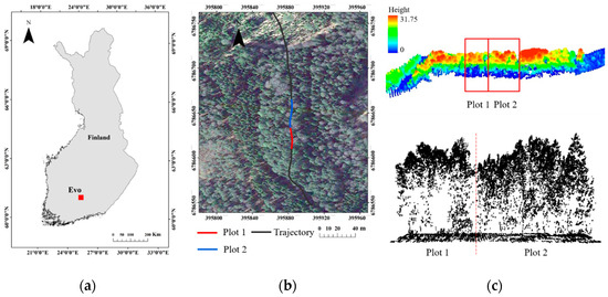
Figure 4.
(a) Location of the test site, Evo in southern Finland; (b) trajectory of data acquisition in the test site (black line) and the selected plot 1 (red line), plot 2 (blue line), in addition, the image only serves as a base map to illustrate the forest conditions and does not mean that it was collected at the same time; (c) the lidar point cloud of the two plots.
4.1.2. Profile Radar Data
The Ku-band FM-CW profile radar system, Tomoradar, was used to collect data. The center frequency of Tomoradar is 14 GHz with 163-Hz modulation frequency and the field of view (FOV) is 6°, owing to the beam width of antenna is 3 dB. Tomoradar can receive waveform of four polarization modes (HH, HV, VH, and VV) with 0.15-m range resolution. Since mechanical scanner was not installed, the backscattering signals could be recorded only at normal direction alone the trajectory by Tomoradar. In addition, the footprint of single waveform was determined by the FOV and flight altitude of Tomoradar. The main parameters of Tomoradar are provided in Table 2.
Table 2.
Main parameters of Tomoradar. FM-CW: Frequency Modulated Continuous Wave.
In the selected plots, due to the average flight height being 60 m and the FVO 6°, the footprint-width of Tomoradar was about 6 m. Tomoradar continuously collected waveforms with the spacing between the center points of every two footprints alone track of 0.06 m, owing to the average flight speed of helicopter being 10 m/s. The co- and cross- polarization (HH and HV) Tomoradar waveforms of the selected plots were employed to compared, as reference, with the simulated waveforms of the extended RAPID2 model in this paper. In addition, the vertical profiles of plot 1 and plot 2 consist of 556 waveforms and 797 waveforms, respectively. The vertical profiles of plots for both polarizations are illustrated in Figure 5. Chen et al. provide a detailed description of the data processing [11].
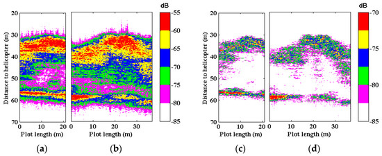
Figure 5.
The Tomoradar vertical profiles of the selected plots in co- and cross- polarization, which are colored with backscattering energy intensity. (a) Co-polarization vertical profile of plot 1; (b) co-polarization vertical profile of plot 2; (c) cross-polarization vertical profile of plot 1; (d) cross-polarization vertical profile of plot 2.
4.1.3. Lidar Data
The lidar data were used to extract forest structure parameters, acquired in the same area during Tomoradar waveform collection, and to reconstruct the 3D scene of the plots in the extended RAPID2 model. The lidar system is a Velodyne VLP-16 laser scanner working with 300,000 pts/s, installed on the same airborne platform, and collecting data simultaneously with Tomoradar. It can generate 16 scan lines uniformly within the FOV of 30°alone, the trajectory and the beam size of transmitted laser pulse is 12.7 mm (horizontal) 9.5 mm (vertical). The main parameters of the lidar are provided in Table 3. For the selected plots, the lidar data were collected with the average point density of about 80 pts/m2. The lidar point cloud of the two plots are shown in Figure 3c.
Table 3.
Main parameters of the lidar
4.2. Generation of 3D Forest Scene
4.2.1. Forest Parameters Acquisition Method
In order to reconstruct the 3D scene of the selected plots in the extended RAPID2 model, the parameters of single trees were extracted from the lidar point cloud. The raw data of lidar were segmented into point cloud of each single tree (Figure 6), after a series of processing using LiDAR360 software (http://www.lidar360.com), such as ground points classification [26], normalization based on ground points, and single tree segmentation based on seed points modified by human-computer interaction, so as to extract the location, height, crown length, and crown width of each single tree in the plots.
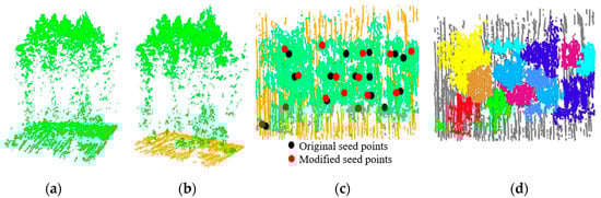
Figure 6.
(a) Raw data of lidar point cloud; (b) normalization based on classified ground points; (c) generation of seed points by layer stacking (black points) and modification of seed points by artificial (red points); (d) illustration of single tree segmentation with seed points.
According to the single tree point clouds and Beer–Lambert law, the LAI of trees could be calculated based on the light intensity at the top and bottom of the canopy and the corresponding extinction coefficient [27]. When applied to point cloud data, the light intensity at the top of the canopy can be regarded as the total number of point clouds reaching the forest, and the bottom light intensity is regarded as the number of point clouds, which reach the ground through the forest canopy [28]. Therefore, the LAIs of each single tree in plots were obtained by the following formula.
where is the number of point clouds reaching the ground and is the total number of point clouds reaching the top of forest canopy.
Lidar cannot produce the detailed parameters of needles and branches. Thus, these parameters were obtained according to literatures [29] and iterative fitting of experiment data. The dielectric constants of components in Ku-band were calculated according to Ulaby [30].
4.2.2. Acquired Forest Parameters and Generated Scenes
Based on point clouds of the segmented trees, there are 21 and 41 trees in plot 1 and plot 2, respectively (Figure 7). Table 4 shows the major structure parameters of the two plots extracted from lidar.
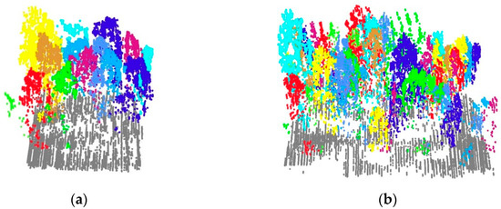
Figure 7.
(a) Single tree segmentation result of plot 1; (b) single tree segmentation result of plot 2.
Table 4.
The major structure parameters of the two plots extracted from lidar.
The main canopy parameters of the plots for simulation are presented in Table 5. The needle length was 5 cm with a diameter of 0.2 cm and the needle zenith angle distribution was set to be uniform. Soil correlation length was 18.75 cm while roughness height was 0.25 cm. Table 6 shows the dielectric constants of components in Ku-band for this study.
Table 5.
The main canopy parameters of the plots for simulation.
Table 6.
The dielectric constants of components in Ku-band.
The 3D scenes of the plots were generated in the extended RAPID2 model utilizing the parameters of single tree and dielectric constant of various components, as described above. The virtual 3D scenes are illustrated in Figure 8.
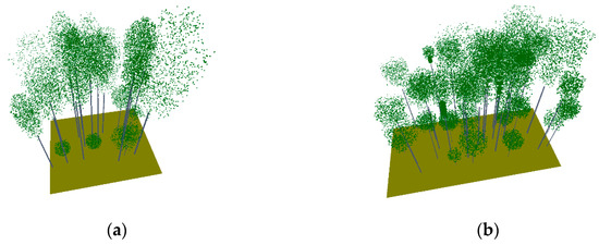
Figure 8.
The virtual 3D scenes in the extended RAPID2: (a) 3D scene of plot 1; (b) 3D scene of plot 2.
4.3. Comparison of Simulation Results
Based on the generated 3D forest scenes, the extended RAPID2 model simulated the profile radar waveforms. To verify the simulation results of the extended RAPID2 model, the Tomoradar waveforms were used as references. To ensure the effectiveness of the comparison, the range resolution of the simulated waveforms has been set to 0.15 m with a footprint-width of 6 m, matching with measured data parametersTo ensure the effectiveness of the comparison, the range resolution of the simulated waveforms has been set to 0.15 m with a footprint-width of 6 m, matching with measured data parameters. In addition, the average waveforms of the two plots at co- and cross- polarization modes were employed for simulated and Tomoradar data in the evaluation. The comparisons between simulated data and Tomoradar data are shown in Figure 9.
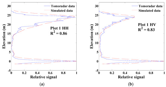
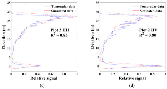
Figure 9.
Comparison between the average waveforms of simulated data (red dashed line) and Tomoradar data (blue solid line): (a) HH polarization of plot 1 (R2 = 0.86); (b) HV polarization of plot 1 (R2 = 0.83); (c) HH polarization of plot 2 (R2 = 0.83); (d) HV polarization of plot 2 (R2 = 0.80).
Figure 9 shows that the modeled average waveforms are in a good agreement with Tomoradar waveforms for both two plots and two polarization modes. The determination coefficients are not less than 0.8. When it comes to the same plot, better consistency was shown at co-polarization, whereas the simulated backscattering was lightly underestimated at cross-polarization. Compared with the average waveforms of Tomoradar, which contained detailed structure in canopy, the simulated waveforms reflected the macro trend of backscattering energy distribution in forest canopies. In addition, the Tomoradar data showed hairy and jagged due to background noise, which did not exist in the simulated data. Therefore, the difference appeared between the simulated data and Tomoradar data, especially at cross-polarization. Small sub-layers were not simulated in canopy (Figure 9d). For the plot with different forest density, the extended RAPID2 model performed better in the thin forest, and their determination coefficients was 0.03 higher than that of in the dense forest for both two polarization modes.
In addition, the extended RAPID2 model could describe the ground waveform accurately with the empirical coefficients (k) of 0.25 and 0.50 in plot 1 and plot 2, respectively, at cross-polarization mode.
5. Sensitivity Analysis of Penetration Depth
The penetration depth of microwave signal generally determines its detection ability of forest vertical structure. Different penetration depth means different contribution sources of scatters. The penetration depth in the canopy could be defined as follows [20]:
where is the total energy reaching the top of the canopy and e is the Euler number. To avoid confusion, it should be noted that the penetration depth does not mean the depth that profile radar can finally reach. Instead, the penetration depth only reflects the position where approximately half of the total energy is accumulated.
A few studies have focused on the influence of canopy structure on penetration depth in the X and L band [20,31,32]. Nevertheless, a more thorough study on the effects of forest density, canopy LAI and branch density on penetration depth would be desirable. It could help to improve the accuracy of forest height estimation and aboveground biomass estimation with a better understanding of the relationship between forest parameters and microwave penetration depth. In addition, sensitivity analysis would interpret effectively the variation trends of the relationships under different forest conditions.
The extended RAPID2 model enables the sensitivity analysis by generating a series of forest scenes. In this paper, the effects of stem density, single tree LAI, crown shape, and twig density on penetration depth in the Ku-band were studied. The contribution of each specified factor was locally checked when other forest parameters were fixed. Table 7 presents the variables and their values that we are concerned about; and the others basic default forest parameters are shown in Table 8. It should be noted that, in this section, the simulated scenes were evenly distributed coniferous forests with a size of 50 m × 50 m, and without overlapping between crowns, which avoids the increasing of leaf density within a crown due to overlapping. The crowns were composed of cone and cylinder, with a randomly oriented leaf angle distribution. The crown shape was defined as the ratio of cylinder part to crown.
Table 7.
Four key variables for sensitivity analysis and their discretized values.
Table 8.
Basic default forest parameters for sensitivity analysis.
Figure 10a–e depict variations in stem density from 200 to 1000 stems/ha with a step of 200 in simulated scenes, where the leaf area index (LAI) of single trees was 3.0. Five groups of forests scenes (500 stems/ha) were generated, which consisted of different LAI values per tree (Figure 10f–j). Next, five kinds of crowns with single tree LAI of 7.0 are shown in Figure 10k–o, forming 500 stems/ha forests scenes, respectively.
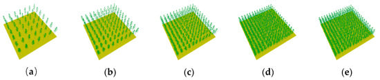
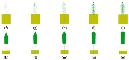
Figure 10.
Virtual scenes for sensitivity analysis on penetration depth: (a–e) with a stem density of 200, 400, 600, 800, 1000 stems/ha when single tree LAI was 3.0 and crown ratio of cylinder part was 70%; (f–j) with a single tree LAI of 1.0, 2.0, 3.0, 5.0, 7.0 when stem density was 500 stems/ha and crown ratio of cylinder part was 70%; (k–o) with a crown ratio of cylinder part of 60%, 70%, 80%, 90%, 100% when stem density was 500 stems/ha and single tree LAI was 7.0.
In addition, five scenes of different twig densities in the crown were also set when stem density was 500 stems/ha, single tree LAI was 3.0, and the crown ratio of cylinder part was 70%. Simultaneously, the branch density was set to 0.2 to 1.8 with a step of 0.4, matching the twig density variation.
For the above-mentioned 20 virtual forest scenes, the profile radar waveforms in Ku-band were simulated by the extended RAPID2 model, and the penetration depths were calculated. Since the vertical resolution of the simulated waveforms was set to 0.15 m, which is consistent with Tomoradar data, the error of penetration depth calculation was not less than 0.15 m. The penetration depth variations of the 20 forest scenes are presented in Figure 11.
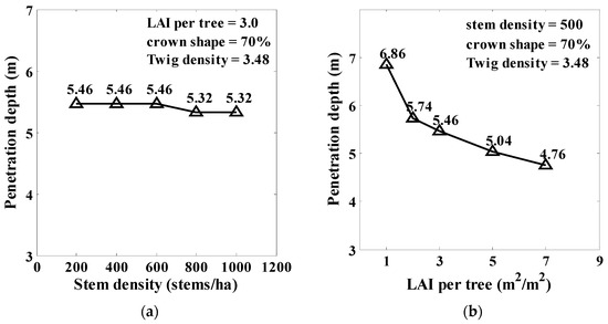
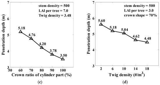
Figure 11.
The penetration depth variations due to the forest scenes vary with (a) stem density when single tree LAI was 3.0, crown ratio of cylinder part was 70%, and twig density was 3.48; (b) single tree LAI when stem density was 500 stems/ha, crown ratio of cylinder part was 70%, and twig density was 3.48; (c) crown ratio of cylinder part when stem density was 500 stems/ha, single tree LAI was 7.0, and twig density was 3.48; (d) twig density when stem density was 500 stems/ha, single tree LAI was 3.0, and crown ratio of cylinder part was 70%.
Figure 11a presents how penetration depth varies with the stem density when other forest parameters are fixed. It can be observed that the penetration depth remained at about 5.46 m, which hardly changed with the increasing of stem density. The penetration of microwave signal tends to be almost not affected by stem density, which is different from previous studies. This may be due to two reasons: firstly, the observation angle of profile radar is nadir-looking, differing to traditional side-looking radar. When the electromagnetic wave is emitted vertically, the interaction occurs in the vertical path, but the stem density mainly determines the number of trees in horizontal direction. Secondly, there was no overlapping between the single tree crowns in these virtual forest scenes; thus, the stem density cannot affect the vertical distribution of needles and twigs within a single tree.
Figure 11b shows the relationship between penetration depth and single tree LAI. The penetration depth decreased with the increasing of single tree LAI. Especially when the LAI increases from 1.0 to 2.0, the value of penetration fell off from 6.86 to 5.74 m. In addition, with the further increasing of the LAI, the penetration depth decreased to 4.76 m smoothly. This obvious variation in penetration reflects the fact that needles contribute the microwave backscattering in Ku-band, and more needles weaken the signal penetration.
The effect of crown shape on penetration depth is shown in Figure 11c. Crown shape was defined as the ratio of the cylinder part to the whole crown. According to the figure, for the same single tree LAI, the larger the proportion of the cylinder part in the crown, the lower the penetration depth. It is understandable that the crown shape determined the spatial distribution of LAI in this study. The increase of the cylinder part of the crown was essentially the increase of LAI at the top of the crown in this experiment (Figure 10k–o). Therefore, we can conclude that the increase of LAI in the microwave propagation path would decrease the penetration depth.
Figure 11d demonstrates the influence of the twig density in the crown on the penetration depth. It can be seen that a gradual decline of penetration from 5.60 to 4.48 m occurred, due to the increasing of twig density in canopy, implying that the twig also contributed to backscattering energy and extensive twigs reduced microwave penetration in the Ku-band.
6. Discussion
In this study, we achieved to simulate the backscattering waveform of profile radar by extending RAPID2 model; thus, helping to understand the interaction between microwave and various forest parameters. Compared with the waveforms of Tomoradar, the extended RAPID2 model worked well in both co- and cross- polarization for dense and thin forests. Further, taking advantage of the extended RAPID2 model, the effects of stem density, single tree LAI, crown shape, and twig density in forests on penetration depth in Ku-band were analyzed. The following sections discuss the results in detail.
6.1. Comparisons of Accuracies in Waveform Simulation
The waveform simulated by the extended RAPID2 model shows different accuracy under different polarization modes and different forest densities. To our knowledge, there were only two previous similar studies on the profile radar simulation, the HUTSCAT waveforms [20,21]. The vertical resolution of the HUTSCAT waveform is 0.68 m. In the simulations of HUTSCAT waveforms, a continuous canopy model, a distributed 2D canopy model, and a 3D canopy model were used separately; and there was gradually weakened underestimation of backscattering at the lower part in canopy [21]. For the 17-meter-high stand in their study, the simulated results agreed well with the HUTSCAT waveforms at the upper part of the canopy (from 8 to 17 m), but between 2 and 8 m, there were still underestimations of several to dozen dB. The specific values of determination coefficient or root mean square error (RMSE) for the simulated waveforms was not given. Compared to HUTSCAT, the simulations of the extended RAPID2 have a better matching to the Tomoradar waveforms, and the determination coefficients were greater than or equal to 0.8 for the two polarization modes and two forest scenes. The vertical resolution of waveform simulated in this paper is 0.15 m.
There are two reasons for the improvement. First, since the extended RAPID2 can generate the scene closing real forest, and the forest parameters were obtained from lidar, the simulated waveforms in this study were better in macro trend. Second, the quality of Tomoradar is higher, for example, the vertical resolution is 0.15 m, which means the simulation in our study can more accurately characterize the backscattering profiles of true forest, but it is possible to make more errors in details as well.
Specifically, for the same forest scene, there was a good agreement of simulated backscattering waveform at co-polarization, while a light underestimation was found at cross-polarization, especially in the denser forest. The similar phenomenon occurred in the previous study, where the profile radar waveforms of Australian pine canopies, aged 30 and 40 years old in X band, were simulated [20]. For the 40-year-old canopy, the simulated waveform, a little more, underestimated the backscattering of the lower part at cross-polarization mode than at co-polarization mode. One explanation for this result is that the cross-polarization signals contain more multiple scattering contributions from the canopy relative to that of co-polarization [33]. In addition, the multiple scattering depends on the density of needles and twigs, which are difficult to determine accurately [22]. Another possible explanation is that the cross-polarization signals suffer from a higher proportion contribution of background noise, because the backscattering intensity of cross-polarization signals is significantly weaker than that of co-polarization. Noise floor of the FM-CW radar is typically determined by the internal reflections. In this study, we had to fix the density of twig, for a crown, without varying from top to bottom, because we did not have the corresponding ground measurement, in addition, background noise caused by internal reflections did not exist in simulations.
For the forest scenes with different densities, better matching of waveform simulation was found in the thin forest plot. On the contrary, the more errors existed in waveform simulation of the dense forest plot, especially in the interior of the multi-layered canopy, and in the lower part of the forest. This could be because the main forest parameters used to construct the virtual scene, such as the number of single trees, the height, and the crown length, etc., were obtained by lidar point cloud data. For lidar, it is hard to detect the detailed information in complex canopy and understory vegetation, due to the mutual shielding of branches and leaves. Zhou et al. compared the canopy height profiles extracted from the Tomoradar waveforms and lidar data; both data were used in this paper [14]. They found that the locations of the canopy height profiles acquired from the lidar were obviously higher than those from the Tomoradar. It also indicates that detection to the details in the lower part of canopy are difficult for lidar, especially in dense forest. To the end, it results in the error of inputs of the extended RAPID2 model and the error of simulation results.
6.2. Sensitive Factors on Penetration Depth
In this study, microwave penetration depth of various forests in Ku-band was concerned, which appeared to be more prominent (3.50 m to 6.86 m) than previous qualitative results for short wavelength SAR (only ‘a few’ meters) [31,34]. This discrepancy is mainly due to the fact that the penetration depth in the previous study was for side-looking radar. For the radar system with the normal incidence, our findings are consistent with the conclusion by Martinez et al. [20] that the penetration depth is several meters in X band. It appeared to be influenced by the density of both needles and twigs in the Ku-band.
A seemingly uncommon finding is that forest stem density was less impacted on profile radar penetration. This is due to the fact that there was no cross between tree crowns in the nadir direction. Despite the increasing of stem density, the volume density of needles or twigs on the path of microwave transmission (such as nadir incidence) did not change significantly. The slight change on penetration is mainly because of the field of view (FOV = 6 degrees), where the off-nadir directions still exist for the profile radar. When the stem density increases to a certain degree, there will be a slight change of backscattering energy in off-nadir directions, leading to the change of penetration depth. Figure 11a presents the phenomenon and provides specific values. Similarly, the sensitivity to stem density should be higher for side-looking radar, since higher stem density means higher density of needles and twigs on the path of off-nadir incidence. Several studies have proven this point: penetration depth decreased significantly with the increasing of stem density for side-looking radar [31,32].
To further verify this view, we have realized the variation of needle density on the profile radar observation path by changing the crown shape, namely the ratio of the cylinder part of the crown. As shown in Figure 11c, the results indicated an obvious decreasing trend of penetration depth with the increasing needle density on observation path. Thus, it can be seen that only the change of the density of the components, such as needles, with scattering contribution in the observation path, can cause the change of microwave penetration depth.
6.3. Advantages and Limitations of Our Approach
The current study has a number of strengths over previous research in terms of exploring the interaction between microwave scattering and forests. Firstly, the scenes are generated with forest parameters obtained from the lidar data, which were acquired simultaneously with Tomoradar waveform, thus improving the consistency of the scenes. Secondly, the waveform simulations have higher timing and ranging resolution, which shows the backscattering energy distribution in vertical direction of forest plots clearly. Third, penetration depth of profile radar in Ku-band tends to be more important (from 3.50 to 6.86 m); and sensitivity of a few forest parameters to penetration depth has been analyzed quantitatively.
Despite the strengths of the study, there are also some limitations. These limitations are primarily related to the parameters of canopy that were set according to previous studies. It is possible that the inaccuracy of canopy parameters could produce the errors of canopy scattering. However, it is difficult to measure the diameter and length of numerous branches and twigs accurately even if in-situ measurement could be carried out. On the contrary, using the classical canopy parameters directly is beneficial to a more consistent comparison with the previous study. In fact, in complex vegetation canopies, the best parameter setting might be the average value of the different parameters, as long as the simulated waveform is fitted well. Hence, the uncertainty of canopy parameters is acceptable during the simulation of profile radar waveform.
6.4. Inspirations from Profile Radar to Explore SAR Ranging
It is worth noting that before getting a desired simulation of the profile radar waveform, only the observation direction, the ground surface backscattering, and the output format were modified in the process of extending RAPID2 model, while the scattering process of each component within the crown has not been changed. Similarly, Floury et al. and Martinez et al. utilized the same MIT/CESBIO backscattering model [18] to realize the SAR data simulation [19] and profile radar waveform simulation [20] of forest canopy. These findings support our basic hypothesis that there is no difference in the scattering process of the components within the crown between the side-looking radar and profile radar. Therefore, it tends to suggest that it is possible to obtain the backscattering energy distribution of the forest in single track SAR image by making statistics of the range direction within a certain window and integrating it to the direction perpendicular to the ground. Of course, it requires that the data have a very high range resolution (e.g., less than 0.5 m) relative to the height of the forest canopies. By properly setting dielectric constants of background, trunks, branches, and leaves for different frequency radar signals, and calibrating their scattering and extinction functions, the extended RAPID2 model can simulate the profiles for other frequencies (such as L and P band) as well, which are widely used in SAR for forest studies. In the future, the vertical structure information of the forest contained in profile radar waveform and single track SAR data could be compared. Further, the degree to which the single track SAR data obtains the vertical structure of the forest and its corresponding conditions could be studied, so that it can be better used to estimate forest parameters.
7. Conclusions
In this study, the RAPID2 model has been extended to simulate the profile radar waveform of boreal forest, which offers a better understanding of the interaction between the microwave signals and forest structures. A good agreement has been found at both co- and cross- polarization between the simulated and Tomoradar profiles. The determination coefficients were greater than or equal to 0.8 for the two polarization modes and two forest scenes.
To our knowledge, the extended RAPID2 is the first shared 3D radiative transfer model realizing the backscattering simulation of optical, thermal infrared, lidar, side-looking radar, and profile radar based on the unified scene and input parameters. Thus, it will be a wonderful tool for multi-source data fusion research. In addition, our study presents a quantitative assessment on Ku-band penetration in forests, which may widen the use of profile radar data.
Moreover, it is a remarkable fact that there is no fundamental modification between the profile radar and side-looking radar for the backscattering calculation of canopy components, which means that it has potential to obtain the backscattering energy distribution of forest to a certain extent by using single track SAR data. In our next study, we will gain insight into how best to reflect forest vertical structure information with single track SAR data. Some forest growth models, such as the Formind model and Zelig model, will be combined with the extended RAPID2, to make the setting of the forest scene in the model more biologically significant.
Author Contributions
K.D. and H.H. modified the program of the RAPID2 model; Y.Z. estimated the tree LAIs with lidar data; Z.F. and T.H. completed the pre-processing of the Tomoradar and lidar data; Y.C. and J.H. instructed data collection and analysis, reviewed the paper; K.D. analyzed the data; K.D. wrote the paper; H.H. reviewed the paper. All authors have read and agreed to the published version of the manuscript.
Funding
This research was supported by National Natural Science Foundation of China: 41971289.
Acknowledgments
Chinese Academy of Science (181811KYSB20160040), Shanghai Science and Technology Foundations (18590712600) and Beijing Municipal Science and Technology Commission (Z181100001018036), Jihua Lab (X190211TE190) are acknowledged. Additionally, the author also gratefully acknowledges the financial support from Academy of Finland projects “Estimating Forest Resources and Quality-related Attributes Using Automated Methods and Technologies” (Academy decision 334830).
Conflicts of Interest
The authors declare no conflict of interest.
References
- Rauste, Y. Multi-temporal JERS SAR data in boreal forest biomass mapping. Remote Sens. Environ. 2005, 97, 263–275. [Google Scholar] [CrossRef]
- Martinez, J.; Le Toan, T. Mapping of flood dynamics and spatial distribution of vegetation in the Amazon floodplain using multitemporal SAR data. Remote Sens. Environ. 2007, 108, 209–223. [Google Scholar] [CrossRef]
- Fu, H.; Wang, C.; Zhu, J.; Xie, Q.; Zhang, B. Estimation of Pine Forest Height and Underlying DEM Using Multi-Baseline P-Band PolInSAR Data. Remote Sens. 2016, 8, 820. [Google Scholar] [CrossRef]
- Long, J.; Lin, H.; Wang, G.; Sun, H.; Yan, E. Mapping Growing Stem Volume of Chinese Fir Plantation Using a Saturation-based Multivariate Method and Quad-polarimetric SAR Images. Remote Sens. 2019, 11, 1872. [Google Scholar] [CrossRef]
- Tebaldini, S.; Rocca, F. Multibaseline Polarimetric SAR Tomography of a Boreal Forest at P- and L-Bands. IEEE Trans. Geosci. Remote Sens. 2012, 50, 232–246. [Google Scholar] [CrossRef]
- Dinh, H.T.M.; Thuy, L.T.; Rocca, F.; Tebaldini, S.; Villard, L.; Rejou-Mechain, M.; Phillips, O.L.; Feldpausch, T.R.; Dubois-Fernandez, P.; Scipal, K.; et al. SAR tomography for the retrieval of forest biomass and height: Cross-validation at two tropical forest sites in French Guiana. Remote Sens. Environ. 2016, 175, 138–147. [Google Scholar]
- El Moussawi, I.; Ho Tong Minh, D.; Baghdadi, N.; Abdallah, C.; Jomaah, J.; Strauss, O.; Lavalle, M.; Ngo, Y. Monitoring Tropical Forest Structure Using SAR Tomography at L- and P-Band. Remote Sens. 2019, 11, 1934. [Google Scholar] [CrossRef]
- Cazcarra-Bes, V.; Tello-Alonso, M.; Fischer, R.; Heym, M.; Papathanassiou, K. Monitoring of Forest Structure Dynamics by Means of L-Band SAR Tomography. Remote Sens. 2017, 9, 1229. [Google Scholar] [CrossRef]
- Hallikainen, M.; Hyyppä, J.; Haapanen, J.; Tares, T.; Ahola, P.; Pulliainen, J.; Toikka, M. A Helicopter-Borne Eight-Channel Ranging Scatterometer for Remote Sensing: Part I: System Description. IEEE Trans. Geosci. Remote Sens. 1993, 31, 161–169. [Google Scholar] [CrossRef]
- Hyyppä, J.; Hallikainen, M. A Helicopter-Borne Eight-Channel Ranging Scatterometer for Remote Sensing: Part 11: Forest Inventory. IEEE Trans. Geosci. Remote Sens. 1993, 31, 170–179. [Google Scholar] [CrossRef]
- Chen, Y.; Hakala, T.; Karjalainen, M.; Feng, Z.; Tang, J.; Litkey, P.; Kukko, A.; Jaakkola, A.; Hyyppa, J. UAV-Borne Profiling Radar for Forest Research. Remote Sens. 2017, 9, 58. [Google Scholar] [CrossRef]
- Piermattei, L.; Hollaus, M.; Milenkovic, M.; Pfeifer, N.; Quast, R.; Chen, Y.; Hakala, T.; Karjalainen, M.; Hyyppa, J.; Wagner, W. An Analysis of Ku-Band Profiling Radar Observations of Boreal Forest. Remote Sens. 2017, 9, 1252. [Google Scholar] [CrossRef]
- Feng, Z.; Chen, Y.; Hyyppa, J.; Hakala, T.; Zhou, H.; Wang, Y.; Karjalainen, M. Estimating Ground Level and Canopy Top Elevation With Airborne Microwave Profiling Radar. IEEE Trans. Geosci. Remote Sens. 2018, 56, 2283–2294. [Google Scholar] [CrossRef]
- Zhou, H.; Chen, Y.; Feng, Z.; Li, F.; Hyyppa, J.; Hakala, T.; Karjalainen, M.; Jiang, C.; Pei, L. The Comparison of Canopy Height Profiles Extracted from Ku-band Profile Radar Waveforms and LiDAR Data. Remote Sens. 2018, 10, 701. [Google Scholar] [CrossRef]
- Attema, E.P.W.; Ulaby, F.T. Vegetation modeled as a water cloud. Radio Sci. 1978, 13, 357–364. [Google Scholar] [CrossRef]
- KARAM, M.A.; FUNG, A.K. Electromagnetic scattering from a layer of finite length, randomly oriented, dielectric, circular cylinders over a rough interface with application to vegetation. Int. J. Remote Sens. 1988, 9, 1109–1134. [Google Scholar] [CrossRef]
- Ulaby, F.; Sarabandi, K.; McDonald, K.; Whitt, M.; Dobson, M.C. Michigan microwave canopy scattering model. Int. J. Remote Sens. 1990, 11, 1223–1253. [Google Scholar] [CrossRef]
- HSU, C.C.; HAN, H.C.; SHIN, R.T.; KONG, J.A.; BEAUDOIN, A.; LE TOAN, T. Radiative transfer theory for polarimetric remote sensing of pine forest at P band. Int. J. Remote Sens. 1994, 15, 2943–2954. [Google Scholar] [CrossRef]
- Floury, N.; Picard, G.; Toan, T.L.; Kong, J.A.; Castel, T.; Beaudoin, A.; Barczi, J.F. On the coupling of backscatter models with tree growth models: 2) RT modelling of forest backscatter. In Proceedings of the 1997 IEEE International Geoscience and Remote Sensing Symposium (IGARSS 1997), Singapore, 4–9 August 1997; pp. 787–789. [Google Scholar]
- Martinez, J.M.; Floury, N.; Toan, T.L.; Beaudoin, A.; Hallikainen, M.T.; Makynen, M. Measurements and modeling of vertical backscatter distribution in forest canopy. IEEE Trans. Geosci. Remote Sens. 2000, 38, 710–719. [Google Scholar] [CrossRef]
- Picard, G.; Toan, T.L.; Quegan, S. A three-dimensional radiative transfer model to interpret ranging scatterometer measurements from a pine forest. Waves Random Media. 2004, 14, S317–S331. [Google Scholar] [CrossRef]
- Huang, H.; Zhang, Z.; Ni, W.; Chai, L.; Qin, W.; Liu, G.; Xie, D.; Jiang, L.; Liu, Q. Extending RAPID model to simulate forest microwave backscattering. Remote Sens. Environ. 2018, 217, 272–291. [Google Scholar] [CrossRef]
- Huang, H.; Qin, W.; Liu, Q. RAPID: A Radiosity Applicable to Porous IndiviDual Objects for directional reflectance over complex vegetated scenes. Remote Sens. Environ. 2013, 132, 221–237. [Google Scholar] [CrossRef]
- Fung, A.K.; Li, Z.; Chen, K.S. Backscattering from a randomly rough dielectric surface. IEEE Trans. Geosci. Remote Sens. 1992, 30, 356–369. [Google Scholar] [CrossRef]
- Oh, Y.; Sarabandi, K.; Ulaby, F.T. An empirical model and an inversion technique for radar scattering from bare soil surfaces. IEEE Trans. Geosci. Remote Sens. 1992, 30, 370–381. [Google Scholar] [CrossRef]
- Zhao, X.; Guo, Q.; Su, Y.; Xue, B. Improved progressive TIN densification filtering algorithm for airborne LiDAR data in forested areas. ISPRS-J. Photogramm. Remote Sens. 2016, 117, 79–91. [Google Scholar] [CrossRef]
- Monsi, M. On the Factor Light in Plant Communities and its Importance for Matter Production. Ann. Bot. 2004, 95, 549–567. [Google Scholar] [CrossRef]
- Richardson, J.J.; Moskal, L.M.; Kim, S. Modeling approaches to estimate effective leaf area index from aerial discrete-return LIDAR. Agric. For. Meteorol. 2009, 149, 1152–1160. [Google Scholar] [CrossRef]
- Karam, M.A.; Amar, F.; Fung, A.K.; Mougin, E.; Lopes, A.; Le Vine, D.M.; Beaudoin, A. A microwave polarimetric scattering model for forest canopies based on vector radiative transfer theory. Remote Sens. Environ. 1995, 53, 16–30. [Google Scholar] [CrossRef]
- Ulaby, F. Microwave Dielectric Spectrum of Vegetation Part II: Dual-Dispersion Model. IEEE Trans. Geosci. Remote Sens. 1987, 25, 550–557. [Google Scholar] [CrossRef]
- Askne, J.I.H.; Persson, H.J.; Ulander, L.M.H. On the Sensitivity of TanDEM-X-Observations to Boreal Forest Structure. Remote Sens. 2019, 11, 1644. [Google Scholar] [CrossRef]
- Ni, W.; Zhang, Z.; Sun, G.; Guo, Z.; He, Y. The Penetration Depth Derived from the Synthesis of ALOS/PALSAR InSAR Data and ASTER GDEM for the Mapping of Forest Biomass. Remote Sens. 2014, 6, 7303–7319. [Google Scholar] [CrossRef]
- Anthony Freeman, S.L.D. A Three-Component Scattering Model for Polarimetric SAR Data. IEEE Trans. Geosci. Remote Sens. 1998, 36, 963–973. [Google Scholar] [CrossRef]
- Garestier, F.; Dubois-Fernandez, P.C.; Papathanassiou, K.P. Pine forest height inversion using single-pass X-band PolInSAR data. IEEE Trans. Geosci. Remote Sens. 2008, 46, 59–68. [Google Scholar] [CrossRef]
© 2020 by the authors. Licensee MDPI, Basel, Switzerland. This article is an open access article distributed under the terms and conditions of the Creative Commons Attribution (CC BY) license (http://creativecommons.org/licenses/by/4.0/).