Article

Non-locally Enhanced Feature Fusion Network for Aircraft Recognition in Remote Sensing Images

1
Key Laboratory for Parallel and Distributed Processing, Changsha 410005, China
2
College of Computer, National University of Defense Technology, Changsha 410005, China
*
Author to whom correspondence should be addressed.
Remote Sens. 2020, 12(4), 681; https://doi.org/10.3390/rs12040681
Submission received: 5 December 2019 / Revised: 16 January 2020 / Accepted: 21 January 2020 / Published: 19 February 2020

Abstract

:
Aircraft recognition has great application value, but aircraft in remote sensing images have some problems such as low resolution, poor contrasts, poor sharpness, and lack of details caused by the vertical view, which make the aircraft recognition very difficult. Especially when there are many kinds of aircraft and the differences between aircraft are subtle, the fine-grained recognition of aircraft is more challenging. In this paper, we propose a non-locally enhanced feature fusion network(NLFFNet) and attempt to make full use of the features from discriminative parts of aircraft. First, according to the long-distance self-correlation in aircraft images, we adopt non-locally enhanced operation and guide the network to pay more attention to the discriminating areas and enhance the features beneficial to classification. Second, we propose a part-level feature fusion mechanism(PFF), which crops 5 parts of the aircraft on the shared feature maps, then extracts the subtle features inside the parts through the part full connection layer(PFC) and fuses the features of these parts together through the combined full connection layer(CFC). In addition, by adopting the improved loss function, we can enhance the weight of hard examples in the loss function meanwhile reducing the weight of excessively hard examples, which improves the overall recognition ability of the network. The dataset includes 47 categories of aircraft, including many aircraft of the same family with slight differences in appearance, and our method can achieve 89.12% accuracy on the test dataset, which proves the effectiveness of our method.

1. Introduction

With the development of space technology, the remote sensing image has become an effective means to survey and monitor resources, environment, urban layout, and traffic facilities, playing an increasingly important role in these fields. As a subtask of remote sensing image processing, aircraft recognition is of great practical demand and application value. In our study, a remote sensing dataset with 47 types of aircraft is collected from GoogleEarth, and many types belong to the same family with very slight differences between them. Therefore, our research is a fine-grained recognition task of aircraft in remote sensing images, which is very challenging.
On the one hand, aircraft recognition in remote sensing images is more difficult than in ordinary optical images. Generally, remote sensing images of aircraft are acquired at different times and on different platforms, and the light condition, atmospheric transparency, and sensor performance will cause great differences in the imaging effect. Compared with ordinary optical images, remote sensing images have their own unique characteristics which cause difficulties in image recognition: (1) The size of aircraft is generally tens of meters, so the aircraft has only a few pixels in the remote sensing image with low resolution. (2) Weather conditions have a great impact on the image, especially atmospheric damping, diffusion and scattering may reduce contrasts and sharpness considerably. (3) In addition, due to the limitation of the vertical view, many details of aircraft in the vertical direction are occluded. These factors will make it difficult to recognize the type of aircraft.
On the other hand, because there are many kinds of aircraft and the differences between them are subtle, aircraft recognition in remote sensing images is much more challenging. Our dataset includes 47 types of aircraft, to our best knowledge, this is the aircraft recogniton research with the most types of aircraft. By contrast, 7 kinds of aircraft are studied in Reference [1], while 8 kinds of aircraft in Reference [2] and 10 kinds of aircraft in Reference [3]. Even in Reference [4], which studies aircraft recognition as a fine-grained classification problem, only uses a dataset of 17 kinds of aircraft. In our dataset, there are not only large categories such as passenger aircraft, transport aircraft, and fighter aircraft but also many subcategories under each category, many of which belong to the same family. The differences between these subcategories are very subtle, such as only a little difference on the engine or empennage, so our research has to distinguish and recognize aircraft from fine-grained features, which make it more difficult.
However, aircraft also have some available attributes, such as symmetrical shape, obvious geometric features, obvious contour edges, and many repetitive structures. Fully exploiting these attributes will be helpful to the aircraft recognition in remote sensing images.
In the early days, traditional aircraft recognition methods are mostly based on manual features by extracting the texture, color, geometry, and other features of the image, and making certain reasoning to classify the aircraft. References [5,6,7] utilize rotation-invariant characteristics to recognize aircraft. These methods use thresholds to segment the overall contour or shape of the target and extract rotation-invariant features, such as Hu moment, Zernike moment, wavelet moment, Fourier descriptor, and scale invariant feature transform (SIFT) [8] for recognition. Dudani et al. [5] utilize Hu moment invariant features extracted from binary images to automatically identify six aircraft types. Liu et al. [6] combine Zernike invariant features with an independent component algorithm for aircraft recognition. Zhang et al. [7] first use contour tracking technology to eliminate noise, and then use moment invariants to identify the type of aircraft. Hsieh et al. [9] propose a hierarchical classification algorithm based on four different features: wavelet transform, Zernike moment, distance transform, and bitmap. Some methods are based on template matching technology [10,11,12], they utilize the extracted features to match the parametric shape templates. Ge et al. [11] propose a coarse-to-fine process. In the coarse stage, the pose of aircraft is roughly estimated by a single template matching with a defined score criterion, and in the fine stage, a parametric shape model is derived by applying principal part analysis and kernel density function. An et al. [12] propose a new idea to address the aircraft type recognition problem by aircraft’s landmark as a template. In addition to the above methods, there are also a few recognition methods [9,13] that estimate the direction first after binarization and then recognize the types of aircraft, which actually takes advantage of aircraft shape characteristics, such as symmetry. However, these methods rely heavily on handcrafted features, thus lack generalization and discriminative representation ability, which are very important when there are many categories and the differences between categories are subtle.
In recent years, deep learning has achieved great success and developed many excellent neural networks such as Alexnet [14], VGG [15], ResNet [16], which are widely used in image processing fields such as classification, detection, and segmentation. Because of its better fitting ability and robustness, more and more remote sensing images of aircraft begin to be processed and recognized by deep neural networks. Henan et al. [17] use the multilayer perceptron for aircraft identification. Fang et al. [18] remove the interference area and leave the suspended target area in the image using the contour tracing method, normalizing moment invariants of the aircraft by extracting them from the sample, then training the BP neural network for the recognition of the aircraft. Diao et al. [19] attempted to utilize thedeep belief network (DBN) to solve the aircraft recognition task. Given a training set of images, a pixel-wise unsupervised feature learning algorithm is utilized to train a mixed structural sparse restricted Boltzmann machine (RBM). An et al. [12] propose a new idea to address the aircraft type recognition problem by the aircraft’s landmark detection, and use a convolutional neural network called the vanilla network for all landmark regressions. Zuo et al. [20] use a convolutional neural network (CNN) for semantic segmentation, and then put the segmented aircraft mask into the classification algorithm. Zhang et al. [2] train a conditional generation of adversarial network from which the multi-scale characteristics of aircraft can be extracted. Fu et al. [4] adopt a multi-class activation map to locate the aircraft in the image and use a mask filter to eliminate interference in the original image.
In the field of image processing, self-similarity in an image has received growing interest. Perceptual grouping follows some principles, such as the proximity and the similarity to extract groups from initial primitives (such as edges and curves), organize them into sets that have similar "perceptual" content, and use the sets for recognition. Kim et al. [21] propose a hierarchical approach to extracting lines and polygons in digital images based on perceptual grouping. Randall et al. [22] propose a Hierarchical Cluster Model to extract object symmetries from a digital image. Michaelsen et al. [23] propose a method for building recognition in high-resolution SAR images based on perceptual grouping, which make use of symmetry and repetitive similar structure in remote sensing images. Bag of visual words model is another way to exploit similarity, which cluster similar visual descriptors together to form a visual vocabulary. Csurka et al. [24] assign patch descriptors to a set of predetermined clusters, construct a bag of keypoints, which counts the number of patches assigned to each cluster, and then train multi-class classifiers using the bags of keypoints as feature vectors. Batista et al. [25] propose a technique based on a bag-of-keypoints representation to identify images containing buildings in the APM photographic collection. The self-correlation matrix of the image is a simple and straightforward method to model the correlation between long-distance pixels. Des et al. [26] first propose a non-local denoising algorithm based on image self-correlation. References [27,28,29] use non-local means algorithms to remove noise in remote sensing images such as hyperspectral images and radar images.
Inspired by the process of human visual recognition, when the differences between categories are very subtle, we need to locate some important parts in the object firstly, and then carefully observe the subtle features inside the parts. Zhang et al. [30] utilize Selective Search [31] algorithm and R-CNN [32] to locate the head and body of birds in the sub-classification task of 200 species of birds [33], but Selective Search algorithm consumes a lot of computational resources. Huang et al. [34] adopt a full convolutional network to locate key points on the bird, then take a 6 x 6 size region as the concerned part, and propose a two-stream classification network to encodes object-level and part-level cues simultaneously. Zhou et al. [35] propose a generic technique called class activation mapping (CAM), which enables CNN to locate distinguishing or informative areas on an image without using any bounding box annotations. Peng et al. [36] obtain the saliency map by CAM, which is used as the target-level attention, then the object-part spatial constraints are used to select discriminant parts from the candidate parts.
One of the problems existing in recognition methods for aircraft in remote sensing images based on deep learning is that the long-distance correlation in the aircraft images is not properly utilized to enhance the distinguishing features. They use CNN for feature extraction, but CNN is limited in the receptive field, and can only utilize local information within a certain range, unable to establish the relationship between long-distance pixels, and unable to comprehensively utilize global information. In fact, the long-distance correlation in the aircraft image is very obvious, such as significant object edges, symmetrical wings, recurring engines and so on. To carry out fine-grained classification, it is especially necessary to pay attention to some structures or details of aircraft. However, due to such adverse factors as low resolution, poor contrasts and sharpness, some structures are easy to be neglected by CNN. If there exist some similar structures elsewhere, the use of the correlation between them can enhance such useful structures for classification, suppress interferential and irrelevant information, and reduce the error rate of recognition.
Although perceptual grouping and bag of visual words model are both effective ways to group or cluster similar structures but their representation ability is not as good as that of deep neural network, and it is difficult for them to adjust the weight of the clusters for fine-grained classification. On the other hand, References [27,28,29] use non-local means algorithm to remove noise in remote sensing images, but self-correlation is only used for filtering and denoising, just as a preprocessing method of remote sensing images, and it is not integrated into the training process of deep neural network. Wang et al. [37] introduce non-local operation into the deep neural network for the first time and design a residual non-local module in the video classification task, which makes up for the deficiency of CNN in global information perception. Li et al. [38] use non-local operation to remove the superimposed raindrops on the image and achieve a good effect. In this paper, non-local operation is introduced into neural network for fine-grained classification of aircraft in remote sensing images, so that the network can make full use of the redundant mode in the aircraft image, learn the long-distance correlation of aircraft, and with the guide of loss function, it can gradually focus on the structures and details that are beneficial to classification and suppress other useless features during iterative training.
Another problem existing in recognition methods for aircraft in remote sensing images based on deep learning is that they all treat the aircraft as a whole to extract features, instead of examining detailed features inside its parts. They distinguish only a few types of aircraft, and the differences between categories are relatively obvious. Therefore, the aircraft can be classified correctly by only the overall features, and there is no need for further feature extraction and fusion of the internal details of the parts. However, there are 47 kinds of aircraft in our dataset, especially different subcategories in the same series, many of which are only slightly different from each other, so we must locate the parts of aircraft and distinguish internal details inside the parts subtly.
Although Zhang et al. [30], Huang et al. [34], Zhou et al. [35], and Peng et al. [36] propose some methods for part location, these methods are not suitable for our classification task of aircraft in remote sensing images. Firstly, part localization and cropping methods do not take full advantage of the geometric features of aircraft. Unsupervised localization methods [35,36] generate fuzzy and irregular boundary of parts, easy to contain irrelevant areas, and have poor positioning accuracy. While the supervised localization method [34] adopts a part cropping strategy that is not suitable for aircraft, which takes the key point as the center to crop a box, and so makes the bounding box relatively loose and may include some background. Secondly, when fusing features of each part, some methods [30,36] need to put each part into a separate network for feature extraction, without sharing the feature extractor, while others such as the method [34] have shared the feature extractor, but each part has no chance to set any unique parameters, and cannot be adjusted respectively. In this paper, we address these problems as follows: when locating the parts, according to the geometric features of the aircraft, we align the posture of aircraft and adopt a reasonable cropping strategy to directly crop 5 geometric regions based on key points, so can localize parts accurately and efficiently; when fusing features of each part, we first put the whole image into the shared feature extractor, then crop the corresponding feature sub-maps of each part on the output of the feature extractor, and then add a part full connection layer (PFC) after the feature sub-maps of each part to learn the detailed features inside the part, which cannot only share feature extractor, but also keep the flexibility of each part to adjust independently, so can improve the network’s ability of extracting detailed features.
In this paper, a complete classification framework of aircraft is constructed based on the deep learning method. Firstly, we adopt the CNN feature extractor to obtain the feature map of the original image, and in view of the symmetry, repetitive structure, and obvious geometric shape of the aircraft, we insert a non-locally enhanced module into the feature extractor, which utilizes the self-correlation operation to enhance the effective features for aircraft classification. On this basis, we use key points to crop 5 parts of the aircraft on the feature map, and extract the detailed features of each part by the part full connection layer (PFC), and then integrated the features of each part by the combined full connection layer (CFC) to complete the final classification. The main contributions of this paper include:
(1) As far as we know, our proposed NLFFNet is the first piece of work that attempts to incorporate non-local operations into the remote sensing image processing task based on neural network architecture, which can get the global receptive field by the self-correlation algorithm, and guide the network to pay more attention to the discriminating structures or details, so as to enhance the effective features for classification.
(2) We propose an efficient method for part localization. According to the appearance characteristics of the aircraft, we develop a reasonable cropping strategy, based on which we utilize 5 key points to generate the part masks, and then crop 5 parts by using these masks. On one hand, the acquired parts provide the prerequisite for the subsequent extraction of subtle features inside each part; on the other hand, these parts combine together to form the mask of the whole aircraft, which can eliminate the interference of irrelevant backgrounds.
(3) We realize an efficient part-level feature fusion mechanism. By shared feature extractor, we get the feature map of the original image, and then crop corresponding feature sub-maps of each part, after that the part full connection layer (PFC) is utilized to extract the detail features inside each part, on this basis, we adopt the combined full connection layer (CFC) to fuse features of all parts. In this way, we cannot only share the feature extractor, but also keep the flexibility of each part to adjust independently, and greatly enhance the recognition ability of subtle difference.
(4) By adopting the improved loss function, we increase the weight of hard examples in the loss function and reduce the weight of examples that are too hard to be recognized, such as outliers, so as to improve the overall recognition performance of the network.

2. Proposed Method

As described in Figure 1, the fine-grained aircraft recognition framework consists of four parts: the part detection sub-network, the feature extraction sub-network, the feature fusion sub-network, and the no-locally enhanced module inserted into the feature extraction.
The workflow is as follows:
(1)
we get an image (denote as Image I) from the dataset, and the nose of the aircraft in Image I may be oriented in any direction. We feed Image I into the part detection sub-network, and get 5 key points of the aircraft;
(2)
we utilize the detected key points to correct the posture of the aircraft in Image I (Image I is rotated accordingly), and generate 5 part bounding boxes according to the strategy, as described in Section 2.2.1;
(3)
we feed the rotated Image I into the feature extractor, and get the feature maps of the whole image;
(4)
we map the part bounding boxes generated in Step 2 to the feature maps generated in Step 3, and get the corresponding feature sub-maps of each part;
(5)
we further extract detailed features of each part and then integrate these features, as described in Section 2.2.2.
In addition, according to the long-distance correlation of aircraft image, a non-locally enhanced module is inserted into the feature extractor, which utilizes self-correlation calculation to improve the features that are beneficial to classification.

2.1. Non-locally Enhanced Module

2.1.1. Long-distance Correlation of Aircraft in Remote Sensing Images

The remote sensing image dataset of the aircraft is collected from GoogleEarth. When using imaging from different times and using different equipment, many images are greatly affected by the external environment. Our dataset reflects the real situation of aircraft in remote sensing images.
It can be seen from Figure 2 that the image of the aircraft has obvious geometric features and symmetrical structures, and there are many redundant modes, such as repeated engines and loads, so there is obvious strong correlation information between the long-distance pixels, this characteristic is of great value for aircraft recognition. At the same time, we find that some structures or details are difficult to be observed because of low resolution, poor contrasts and sharpness (as show in Figure 2). These structures or details may be right the differences between aircraft, if similar structures happen to exist elsewhere, correlation between them can guide neural network to pay more attention to these structures and enhance these effective structures and details.

2.1.2. Principle of Non-locally Enhanced Operation

In our processing framework, we utilize the front part of VGG19 [15] as the feature extractor. The input image size is 224 × 224 × 3 , after multiple convolution and pooling operations, output the feature map with size of 14 × 14 × 512 . Convolution operation in the extractor is a kind of local operation, the output value of each position is obtained by convolution calculation between kernel and the local pixels. Convolution operation assumes that adjacent pixels have a strong correlation, while the correlation of pixels with a long distance is weak. However, there is an obvious correlation of long-distance correlation in the remote sensing images of the aircraft, therefore, non-locally enhanced operation should be adopted in aircraft recognition task.
Non-locally enhanced operation is essentially a self-attention mechanism, and its basic principle is to construct the model’s long-distance dependence by a triple (key, query, value): obtain the corresponding attention weight by dot product between key and query, and then multiply the weight and value to get the final output. It is formalized as follows:
y i = 1 C ( x ) j f ( x i , x j ) g ( x j )
and f ( x i , x j ) is defined as
f ( x i , x j ) = e θ ( x i ) T ϕ ( x j )
where x and y denote the input and output, i and j are the coordinates of pixels, the value range of j is any coordinate in the image. C ( x ) is a normalized constant, f ( . ) is a two-input function used to construct the correlation information between point i and point j, g ( . ) is a single input function to calculate the influence of point j on point i, x i corresponds to the query in the triple, x j corresponds to the key, and g ( x j ) corresponds to the value, while θ and ϕ denote the embedding of query and key respectively. The summation operation is to synthesize the influence of all other pixels on x i (query).
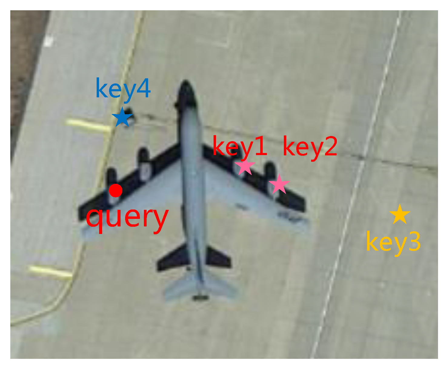
As shown in Figure 3, key1 and key2 have a high similarity to the query, while key3 and key4 have a low similarity to the query. The weight factor f ( q u e r y , k e y 1 ) and f ( q u e r y , k e y 2 ) are correspondingly high, so the output value at the coordinate of the query point can be enhanced by the contribution of high-correlation pixels such as key1 and key2.

2.1.3. The Realization of Non-locally Enhanced Module

The left middle part of Figure 1 briefly depicts the non-locally enhanced module. The input of this module can be any feature layer in the neural network, and the output is exactly the same size as the input, therefore, the module can be inserted into any position in the network without changing the original network. This module adopts residual structure, which makes the gradient of self-correlation operation more easily propagating in the network.
Figure 4 shows the internal calculation process of non-locally enhanced operation. Before calculating the correlation coefficient f ( x i , x j ) , three embeddings are obtained respectively, so that the module has one more chance to adjust before calculating the correlation coefficient, which enable the network to enhance or suppress features more flexibly.
When faced with large size feature map, correlation operation will lead to large-scale matrix calculation. As a compromise, the feature map can be sliced and calculated separately, and then the parts can be combined together, as shown in Figure 5. In Section 3.5, we need to perform non-locally enhanced operation on the feature map output by conv1_2, but the size of the feature map is 112 × 112 , and the computational cost is too large. We adopt this strategy: firstly, divide the 112 × 112 feature map into four sub-maps with size of 56 × 56 ; secondly, perform non-locally enhanced operation on each sub-maps, refer to Figure 4, the matrix calculation cost of each sub-map is 1/16 of the feature map with size of 112 × 112 , and the total calculated cost of the four sub-maps can be reduced to a quarter; thirdly, combine the four outputs of non-locally enhanced operation into a whole feature map with size of 112 × 112 .

2.2. Part-level Feature Fusion

The general classification network directly accesses several full connection layers and a softmax layer after the convolution layers, so as to obtain the probability of each category. In this way, all the pixels in the feature maps of the input image are treated as the same. When there are large differences between classes, the network can distinguish the categories correctly, but in the face of the classification task with slight differences between sub-classes, because the details are easily overwhelmed by irrelevant or distracting information, this processing method is not competent. We need to help the network locate the target and its parts in a certain way, then look for details in these regions. In our method, we generate part’s bounding boxes by key points, extract the subtle features inside each part, improve the network’s ability to distinguish subtle features, and then fuse these features together for classification.

2.2.1. The Strategy to Generate Bounding Boxes of Part

Aircraft are symmetrical in structure and have obvious key points in appearance, so the corresponding parts can be cropped according to the key points. Compared with the part detection method based on proposal boxes, the method based on key points has an obvious advantage, which can reduce the search space and computation. According to the characteristics of the aircraft, five key points are designed, which are located in nose, fuselage, empennage, left-wing and right-wing. We realize key point detection by adopting the method proposed in Reference [39], build a simple and efficient key point detection network based on resnet50 and 3 layers of deconvolution, and use the gaussian heatmap of the key point coordinates as the monitoring information of the network.
According to the appearance characteristics of the aircraft, we develop a set of strategies as the cropping rule of the part. We first correct the aircraft’s posture, we take the line between the nose and fuselage as the datum line and rotate the image to make this line perpendicular to the X-axis.
After posture correction, the size of the aircraft is calculated by the following formula:
W o b j = | x l w i n g x r w i n g |
H o b j = | y n o s e y e m p e n n a g e |
For the parts of nose and fuselage, we offset the key point (Nose or Fuselage) by 5 pixels up as the top boundary of the bounding box and take W o b j e c t / 2 and H o b j e c t / 2 as the width and height of the bounding box. For the empennage, we also take W o b j e c t / 2 and H o b j e c t / 2 as the width and height of the part’s box, take the x coordinate of empennage as the X-axis midpoint of box, took the y coordinate of empennage as a reference, and H o b j e c t *3/8 above the reference, W o b j e c t 1/8 down the reference as the Y-axis interval of the box. The goal of this strategy is to take into account that the left and right horizontal stabilizers are not on the same horizontal plane as the empennage, and most of the areas will be skewed towards the top, this method can better contain the tail area without adding more background areas.
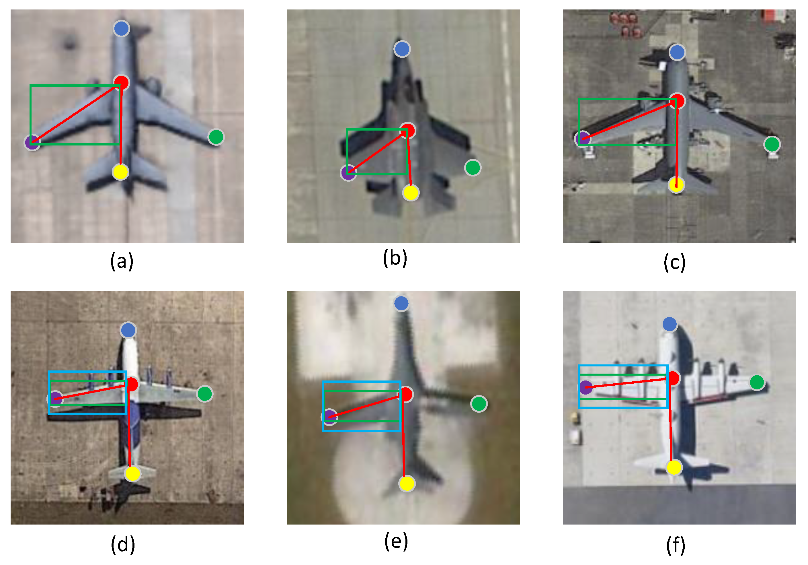
For the bounding box of the wing, we deal with it in two cases according to the angle of wing, where the angle is calculated by the line between fuselage and left-wing (or right-wing) and the line between fuselage and empennage. As shown in Figure 6a–c, when the angle is less than or equal to 60 degrees, draw a rectangular box diagonally with the line connecting fuselage and left-wing or right-wing. Figure 6d–f is the case that the angle is greater than 60 degrees, and in this case, we use the difference between the y-coordinates of Fuselage and left-wing (or right-wing) as the height of the wing (denoted as H w i n g ). When cropping the wing, we reserve H w i n g /2 above and below the wing, so as to capture engines when the wing is spread horizontally. The wing clipping method is formalized as follows:
H w i n g = { α | y w i n g y f u s e l a g e | } = f ( x ) = 2 | y w i n g y f u s e l a g e | , a n g l e > 60 | y w i n g y f u s e l a g e | , a n g l e < = 60
W w i n g = | x w i n g x f u s e l a g e |

2.2.2. Feature Extraction and Feature Fusion of Parts

Firstly, feature maps of each part are obtained by the shared feature extractor based on the part bounding boxes. On this basis, we extract the subtle features inside each part by the part full connection layer(PFC), and then fuse feature maps of each part by the combined full connection layer (CFC), as shown in the right part of Figure 1.
To get the features of each part, the traditional method is to crop the original image, scale the cropped part to meet the input requirements of the feature extraction network, and then obtain the corresponding feature maps of each part through several separate neural networks. However, this method would require a large amount of calculation, specifically 5 times for 5 parts.
In our method, a shared feature extractor is adopted, and transfer the cropping operation of part to the feature maps, to directly obtain the corresponding feature sub-maps of five parts. After multiple convolutions and pooling operations, the original image is transformed from the size of 224 × 224 to the feature map with size of 14 × 14 , and the scaling ratio is 16:1, the coordinates of the part boxes are mapped to the feature map according to this ratio, and then crop the five-part boxes in the shared feature map.
Different parts have different sizes and aspect ratios according to the cropping strategy, to facilitate the subsequent feature fusion, it is necessary to align the feature maps of the cropped parts to the same size. The size range of the cropped parts can be expressed as P s i z e = m × n , 2 < m < 7 , 2 < n < 7 . We adjust these different sizes to 6 × 6 and use bilinear interpolation to obtain the value of each pixel after resize. Bilinear interpolation prevents the precision loss caused by the rounding operation and retains the precision before resize.
We designed a part full connection layer (PFC), which is built by two full connection layers after feature maps of each part, to further extract the details inside the part, which can be formulated as
y i = f ( W i x i ) , i = 1 , 2 , 5
where x i represents the input feature of part i, and y i represents the output feature of part i in the PFC layer, W i represents the weight parameter, and f represents the nonlinear activation function. Especially W i of each part are not shared because we need the network to extract the characteristics of different parts separately.
The PFC layer abandons the irrelevant areas and focuses on the features inside the parts. Each part adopts a separate fully connected parameter matrix, which allows the network to learn individually about each part and further focus on the subtle features that need to be paid attention to inside the part.
After the PFC layer, we adopt the combined full connection layer (CFC) to integrate the information of all parts together. The outputs of the full connection layer of all parts are the same size, which can be concatenated together as the input of the CFC layer. The CFC establish a connection with each node in the PFC, so can model the internal relationship between different parts correctly, which can be formulated as
y = f c ( W c ( i = 0 5 f p ( W i x i ) ) )
where x i represents the input features of part i, W i represents the weight parameters of part i, W c represents the weight parameters of the CFC layer, f c and f p respectively represent the activation function of the CFC layer and the PFC layer, ∑ represent the concat operation between parts, and y represents the final output feature vector of the CFC layer.

2.3. Hard Example Mining

As shown in Figure 7, in the fine-grained recognition task of the aircraft, there exist many hard examples that are difficult to be accurately recognized by the neural network. There are mainly three reasons: firstly, the differences between some categories are subtle; secondly, there are adverse factors such as poor contrasts and sharpness in remote sensing images, which may cause images of different classes to look the same; thirdly, as some labels come from the Internet, inaccurate labels may exist in the dataset.
In general, we use cross-entropy as the loss function of classification, which reflects the degree of difference between the predicted value and the ground truth. The formula is as follows:
H ( p g t , p p r e d ) = i n p g t ( i ) log p p r e d ( i )
where p g t is the ground truth, and p p r e d is the prediction value, n is the number of categories.
When the training reaches a certain stage, most examples can be accurately recognized by the network, while only a few hard examples exist. As mini-batch is used to calculate loss function, the value of loss function is mainly dominated by easy examples, and it is difficult for the network to perceive loss changes caused by difficult examples, so cannot continue to optimize, resulting in an inefficient training process and difficult improvement of classification performance.
To deal with the problem of unbalanced examples in the target detection task, Lin et al. [36] propose focal loss function, adjust the weight of each example in the loss function of mini-batch adaptively according to the predicted value, restrain the easy examples appropriately, and increase the influence of the hard examples, as shown in the Formula (10).
F L ( p g t , p p r e d ) = α i n ( 1 p g t ( i ) p p r e d ( i ) ) ) γ log p p r e d ( i )
In fact, the focal loss has two hyperparameters that require careful adjustments, moreover, it only adjusts the weight according to the difference between the predicted value and the ground truth, but does not reflect the proportion of the hard examples in the mini-batch and does not adapt to the change of data distribution.
In Reference [40], a new gradient coordination mechanism (GHM) is proposed to hedge the incongruity between examples. This method uses the distribution of the gradient norm to reflect the imbalance between hard and easy examples, and the gradient norm is defined as
g = | p g t p p r e d |
which presents the difference between predict value and ground truth, with a value range between 0 and 1. Then, the gradient density function is used to represent the distribution of gradient norm:
G D ( g ) = 1 l ϵ ( g ) k = 1 N δ ϵ ( g k , g )
where N is the total number of examples, g k is the gradient norm of the k-th example, ϵ presents a neighborhood of g, and δ ϵ ( g k , g ) indicates whether g k is distributed in the neighborhood ϵ , and l ϵ ( g ) presents the length of the neighborhood.
With the continuous iteration of training, a large number of gradient norms(g) are concentrated near the 0 value, leaving only a small number of gradient norms away from zero, which mean difficult examples. Although the contribution of an easy example on the gradient is less than that of a hard example, the total contribution of a large number of easy examples can exceed the contribution of a small number of hard examples, and the training process will become inefficient. On the other hand, when the network converges, there may be some too hard examples whose corresponding g value is relatively large, and the density of these g values is slightly higher than that of the normal hard example (because as the training iterates, the g value of the normal hard example is moved to the neighborhood of the 0 value). These hard examples can be considered as outliers because they exist stably even when the model converges. Because the gradient of outliers may be quite different from other common examples, it may affect the stability of the model. If excessive attention is paid to these abnormal examples like focal loss, parameter adjustment will be too large and these outliers will be over-fitted, but at the same time, the fitting ability of other normal examples will be destroyed.
As mentioned above, the reciprocal of gradient density can be used as the loss weight factor of the corresponding example, which can be formulated as follows:
β i = N G D ( g ( i ) )
L G H M - C = 1 N i = 1 N β i L C E ( p i , p i ) = i = 1 N L C E ( p i , p i ) G D ( g i )
where N is the total number of examples, which plays a role of normalization.
The loss function L G H M - C cannot only enhance the influence of hard examples but also restrain the influence of outliers on the loss function. Experimental results show that the loss function can ensure the stability of the model and make it get a better classification result.

3. Experiments and Results

3.1. Dataset

Currently, major public remote sensing image datasets [41,42] contain a few categories with large interclass variance, such as ship, tank, harbor, plane, forest, building. It is easy to distinguish one from another in these datasets, so it can only be used for common classification problems and cannot be used for the study of the fine-grained classification of aircraft.
To study the fine-grained recognition of aircraft, we collected an aircraft dataset from GoogleEarth. We classify the aircraft according to the specific type, rather than roughly divide them into passenger aircraft, transport aircraft, training aircraft, for example. The dataset includes 47 types of aircraft, which as far as we know, is the dataset with most categories of aircraft in remote sensing images. Each type of aircraft has about 17 images, and each image is scaled to the size of 224 × 224 . Sixty percent of them are used as the training set while forty percent as the test set, and the images in the test set never appear in the training set. We use Labelme (a database and web-based tool for image annotation described in Reference [43]) to mark the type information and key points of the image. Each original image is marked with five key points, which are located in the nose, fuselage, tail, left-wing and right-wing. Due to the small number of images, the original images need to be augmented to enhance the generalization performance of the model. We mirror the images, also carried out random translation operations in the upper, lower, left, and right directions, respectively. In the process of data augmentation, coordinate transformation of key points is carried out to ensure the correctness of key points after augmentation. The dataset will be public in the future. Please contact the corresponding author to ask for the state of availability of the dataset.

3.2. Implementation Details

The NLFFNet network is built on TensorFlow 1.10, trained and tested on the operating system Ubuntu 16.4, with an NVIDIA 1080Ti GPU which has 12 GB of memory.
We utilized the conv1_1 to conv5_4 of VGG19 network as a feature extractor. Due to the small amount of data, if we directly start training scratch from random initialization parameters, it is likely that over-fitting will occur. Therefore, we use the pre-trained parameters on imagenet as the initial values of feature extractor, and other network parameters adopted the Xavier initialization. We train the network using SGD optimizer with a mini-batch size of 32, and evaluate the performance of the model with top-1 accuracy as a metric. Cross-entropy is adopted as the loss function and we compare the effects of cross-entropy with focal loss and GHM-C loss function.
Learning rate is a very important parameter in the training process. If too large, the network is prone to gradient explosion, or may not reach the optimal classification results. If too small, the optimization speed of the network is too slow. In the setting of the learning rate, we adopt two basic strategies: (1) Different learning rates are adopted for different parameters. Parameters without pre-training have higher learning rates, while the parameters of the feature extractor, which are loaded from the imagenet pre-training model, have a lower learning rate. (2) The cycle learning rate strategy proposed in Reference [44] is adopted to improve the convergence speed without decreasing the classification accuracy.

3.3. The Results of the Proposed Method

To check the effect of our proposed method, we conduct a series of comparative experiments with other methods. Meanwhile, in order to observe the impact of non-locally enhanced module and part feature fusion (PFF) method on classification results separately, we conduct an ablation experiment.
First, we train some classic CNN networks, including AlexNet, VGG, and Resnet. Due to the small amount of data, we fine-tune based on the pre-training model to ensure the rapid convergence of the model. It can be seen from the results in Table 1 that these classic fine-tuned networks have been able to extract a lot of useful information from remote sensing images of aircraft, and effective classification results can be obtained as long as simple training is conducted. In addition, we also compare with the image segmentation method in Reference [20]. We first train an aircraft segmentation model, then align the direction, and recognize the type of the aircraft. The benefits of this approach in Reference [20] are obvious: it separates the aircraft from the background, reducing the impact of sundries on the ground, and it can be seen from Table 1 that this method has better performance than ordinary CNN networks.
Our proposed method has two main improvements: firstly, we conduct the part-localization and part-level feature fusion according to the geometric feature of the aircraft; secondly, we insert a non-locally enhanced module into the feature extractor to enhance the feature beneficial to classification. To check how much of performance boost these two improvements bring to the network, we make an ablation experiment. First, we add a non-locally enhanced module to the feature extractor, according to our experiment, it is better to put this module in the shallow layer of the network(between conv2_2 and conv3_1). Therefore, in Table 1, we record the classification accuracy when non-locally enhanced module inserting between conv2_2 and conv3_1 of the feature extractor. In addition, we build a part-level feature fusion network based on key points without a non-locally enhanced module, to observe the classification performance improvement brought by the feature fusion method alone. Finally, the non-locally enhanced operation and feature fusion method are assembled together to build a complete fine-grained classification network of aircraft called NLFFNet.
As the proposed method utilizes an additional subnet for key point detection and feature fusion of different selected parts except the baseline extractor module, it must need more computational resources. We use inference time as the criterion of computational cost and evaluate the inference time of the networks with a NVIDIA 1080Ti GPU. The inference time of the baseline feature extractor is 0.11 s, while our proposed method is 0.48 s, our method has a higher computing cost.
The comparison of the accuracy of each method is shown in Table 1, where "Extractor" refers to the feature extractor, "non-local" refers to the non-locally enhanced module, and "PFF" refers to the part-level feature fusion mechanism.

3.4. The Influence of PFF

To observe the influence of part feature fusion on the network, we make a heatmap experiment refer to Reference [45], the steps are as follows:
(1) Firstly, we select the feature maps we are interested in, such as the feature maps obtained after the last convolution (with size of 14 × 14 × 512 , and the following steps are assumed to deal with this size).
(2) The influence of 512 feature maps in the softmax layer must be different, and the weight of each feature map can be calculated by backpropagation. We select the node with the largest softmax value (corresponding to the category with the highest confidence), calculate the gradient of the feature map we were interested in base on backpropagation, and the mean value of the gradient of the feature map is taken as the weight of the feature map.
(3) Multiply each feature map by the weight to get a weighted feature map with a shape of 14 × 14 × 512 , calculate the mean value in the third dimension to get a map with a shape of 14 × 14 , then perform relu activation and normalization.
(4) The heatmap is resized to the shape of the original image, and calculate a weighted sum of the heatmap and the original image, which is available to observation and analysis.
Heatmap can reflect the importance of each region of the image to the classification result, in other words, it can be seen from the heatmap that the network gets a certain classification result because it pays attention to which region of the image mostly.
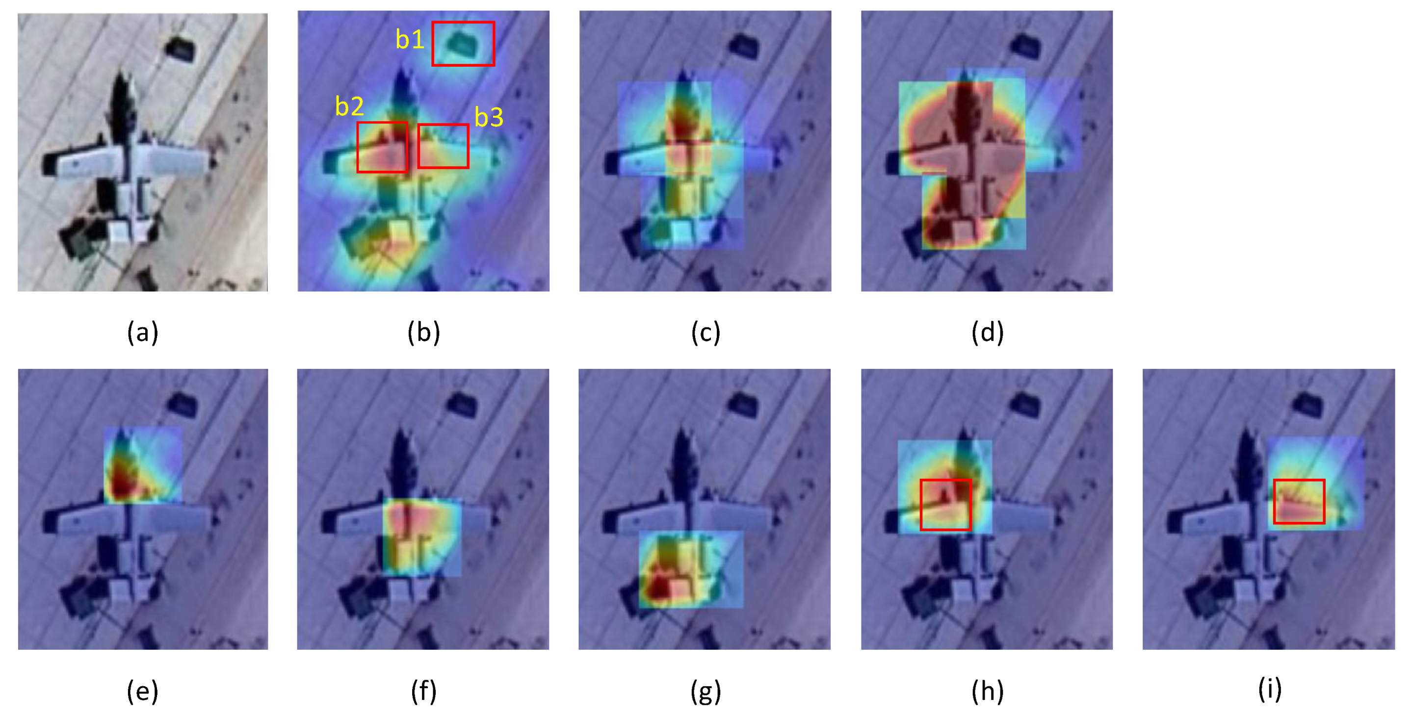
As shown in Figure 8e–i, they represent the heatmap of the nose, fuselage, empennage, left-wing, and right-wing, respectively. Then, the heatmaps of each part were assembled according to their positions in the original image to obtain the concatenated heatmap as shown in Figure 8c. Based on the concatenated heatmap, a threshold is set, and when the heat value is higher than the threshold, it is truncated. Then, all heat values are normalized, and the area beyond the threshold is displayed in a unique brown color to prevent confusion between the background color of the original image and the color of the heatmap, so as to facilitate observation, shown in Figure 8d. It should be noted that in order to facilitate observation, the heatmap is superimposed with the original image. During the superimposition, the pixel value of the original image is multiplied by a weighting factor of 0.4, while the heatmap is multiplied by a weighting factor of 0.6. In addition, the heatmaps of five parts overlapped with a few area when stitching, so the value of the overlaped area get bigger than the real value, and the visualization of the heatmap is automatically generated by calling the applyColorMap function in opencv, which generates a smooth color scheme based on the maximum and minimum values, as a result, the color of each part (as shown in (e)–(i)) is not completely consistent with the color of corresponding parts of sub-diagram (c).
The aircraft in Figure 8 is misidentified before adopting a part-feature fusion method, and it could be correctly recognized after using this method. By comparing (b) and (c) in Figure 8, it can be seen that the part box excludes the interference in the upper right corner. In addition, compared with (h) and box b2 in (b), it can be seen that the network pay more attention to the surface of the wing when without the part-box, while the focused area is obviously shifted to the payload in front of the wing when adding the part box, and the network could extract more detailed information conducive to classification. Similarly, by comparing (i) and box b3 in (b), it can be seen that the payload of the right-wing is paid little attention when without the part-box, and the attention of the right-wing and its payload increase obviously after adding the part-box.
The aircraft in Figure 9 is misidentified before adopting the part-feature fusion method, and it could be correctly recognized after using this method. By comparing (b) and (c) in Figure 9, it can be seen that the part-box excludes the interference on the left side from the attention of the network. In addition, it can be seen from (a) that the left engine and the payload under the left-wing are not obvious due to poor contrasts and sharpness. As shown in box b2 of the sub-diagram (b), the network does not pay attention to the left engine and the payload under the left-wing when there is no part-box, but in the sub-diagram (h), the network obviously pays attention to these details.
A comprehensive comparison of Figure 8 and Figure 9 shows that:
(1)
All part-boxes stitching together actually form a mask of the target, which segments the target from the whole image, and makes the network focus on the target itself, without interference from irrelevant objects and backgrounds outside the target.
(2)
The part full connection layer(PFC) allows the network to learn the details inside each part and to better distinguish the nuances between the subclasses.

3.5. The Influence of Non-locally Enhanced Operation

We try to insert the non-locally enhanced module into different positions of the feature extractor, conduct training respectively, and found that placing it after conv2_2 gets the best effect, as shown in Table 2.
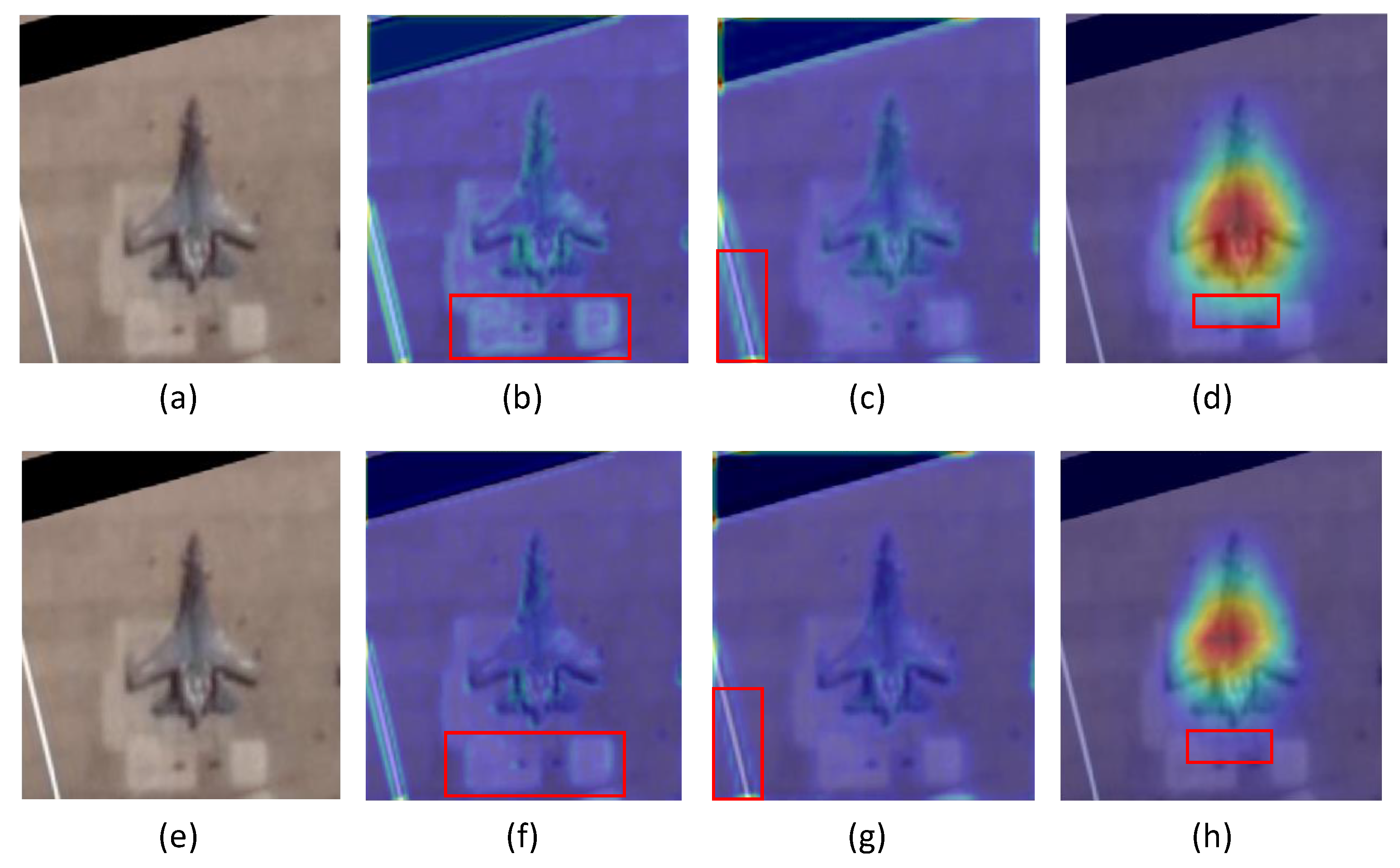
To observe the influence of non-locally enhanced operation, we also draw the heatmaps based on the principle of Grad-Cam [45]. Our non-locally enhanced module is inserted between conv2_2 and conv3_1, so we draw the heatmaps corresponding to conv2_2 and conv3_1. We also draw the heatmap corresponding to conv5_4 to observe the influence of non-locally enhanced operation on the final output of the feature extractor.
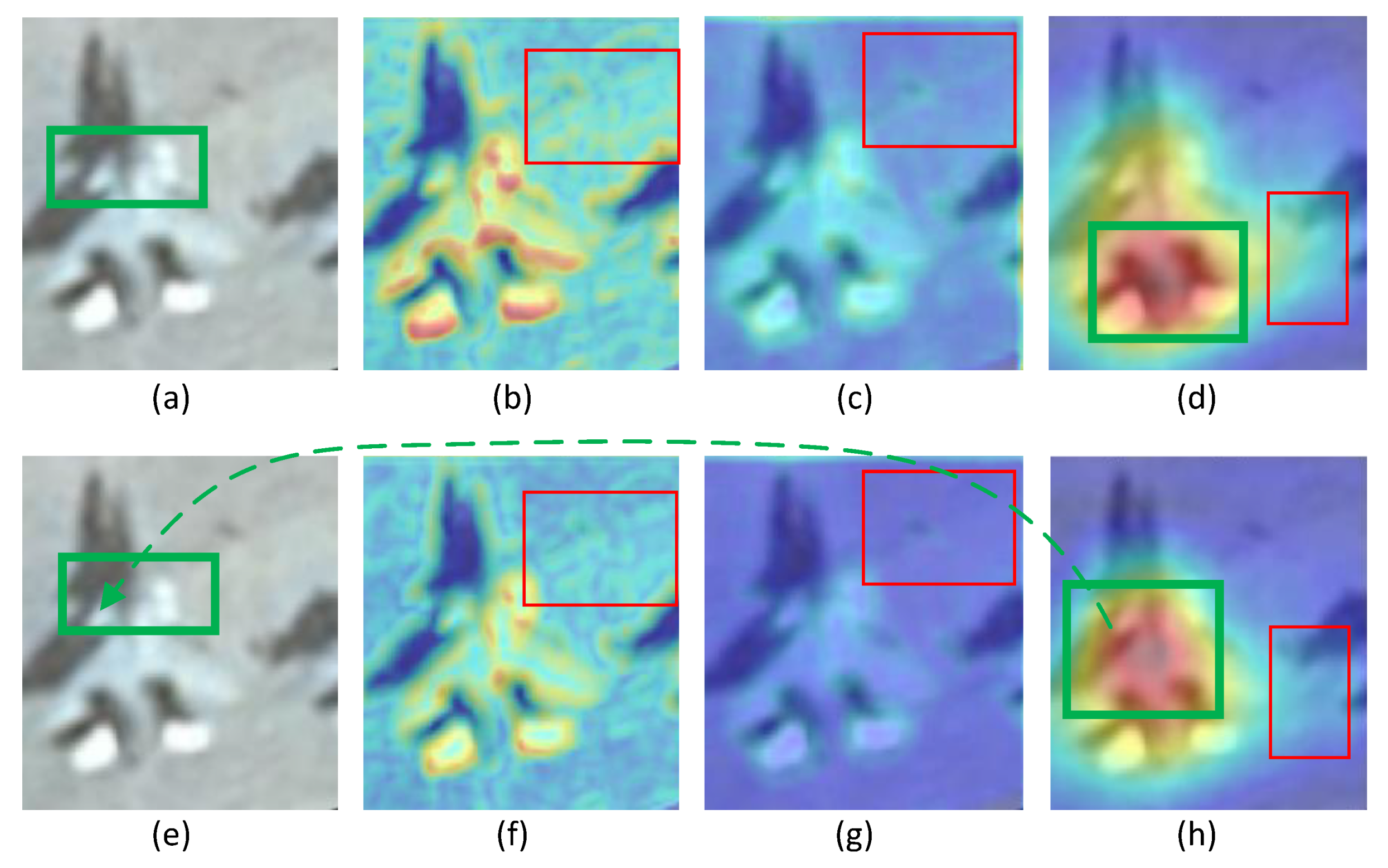
The aircraft Type41 in Figure 10 is misidentified without non-locally enhanced module and can be correctly recognized after the addition of the module. In Figure 10, from the comparison of (b) and (f), as well as a comparison of (c) and (g), it is found that a non-locally enhanced module inhibits the interference of irrelevant objects on the ground. According to the comparison of the green box in (d) and (h), the non-locally enhanced module makes the network pay more attention to the canards(Canards are small delta wings on either side of the cockpit) of Type41, which is a significant feature of Type41 that distinguishes it from Type40(This image happened to be misidentified as Type40 without non-locally enhanced module).
The aircraft Type40 in Figure 11 is misidentified without non-locally enhanced modules, and can be correctly recognized after the addition of non-locally enhanced modules. It is found from (b)(f) in Figure 11 that this module suppress the interference caused by ground plaques. It can also be found from (c),(g) in Figure 11 that the module suppress the interference brought by the ground line.
A comprehensive comparison of Figure 10 and Figure 11 shows that:
(1)
With the addition of a non-locally enhanced module, the focused area on the conv3_1 heatmap is more accurate and concentrated than that without the module, indicating that non-locally enhanced operations could guide the network to focus on effective details and ignore useless features.
(2)
With the addition of a non-locally enhanced module, heatmap of conv2_2 changes significantly compared with that without the module, indicating that all parameters in the neural network are interrelated, and non-locally enhanced modules could not only influence the subsequent feature maps, but also influence the feature maps before the module.
(3)
In the high-level semantic feature maps of conv5_4, the heatmap with non-locally enhanced module is significantly more focused on the aircraft itself and rarely diffuses to irrelevant areas such as the ground, indicating that the effect of the non-locally enhanced module in shallow layers could be effectively transferred to high-level semantics to improve the final presentation and classification ability of the feature extractor.

3.6. The Comparative Experiment of Loss Functions

In the training process of NLFENet, we take cross-entropy as the baseline and compare three different loss functions, aiming at online mining of hard examples by the loss function. The comparison results are shown in Table 3.
According to the formula of focal loss, there are two hyperparameters that can be adjusted. γ is a scalar, which is easy to be adjusted, while α is a vector with a length of 47, which corresponds to the difficult degree of 47 types of aircraft respectively, it is highly dependent on manual experience for careful setting, so it is very difficult to determine the appropriate value. Therefore, only γ has been adjusted in this experiment, whereas α is a vector of all one.
According to the formula of loss function GHM-C, we must calculate the density of the gradient norm, and because the gradient norm g is a continuous distribution between 0 and 1, we should first to discretize it. When programming, we set ϵ = 0.05 and divide 20 intervals between 0-1 and count the number of g values in each interval, thus generating 20 density values ( G D 1 , G D 2 G D j G D 20 ), if the value of g i falls in the k-th interval, we set G D ( g i ) = G D k approximately.
By observing the dataset carefully, it was found that there was a suspicious image of Type1 in the training and test sets, which may be labeled incorrectly, as shown in Figure 12, Figure 13 and Figure 14. In Figure 13a, the image is recognized as type Type1 when cross-entropy is applied, and recognized as type Type27 when GHM-C loss is applied, which indicates that GHM-C loss regards it as an outlier, and the contribution of this outlier is inhibited in the loss function.

4. Discussion

The general image classification methods based on deep learning usually first obtain the feature maps of the original image as a whole through the CNN network, and then classifies them according to the feature maps. However, for the aircraft classification task studied in this paper, due to the high similarity between sub-categories, the difference in the corresponding feature maps is very subtle, so the general methods cannot be competent. We try to solve this problem from two aspects: one is to enhance the structures and details beneficial to classification of the non-locally enhanced operation; the other is to locate and discover the details by feature extraction and feature fusion of parts. In fact, we can also try to convert the original image to a particular feature space, in this kind of space, the similarity between examples of the same category increases (or the distance between them decreases), while the similarity between examples of different categories decrease (or the distance between them increases), so as to improve the clustering performance and improve the discriminant ability of the classifier, which is exactly the method of metric learning.
Deep metric learning combines the feature representation ability of deep learning with the similarity characterization ability of metric learning and realizes the perception from original input to semantic output in an end-to-end manner, which has made important progress in several visual tasks. General deep metric learning includes two aspects: the first is encoding original data to feature vector by the neural network; the second is using loss function to carry out a similarity comparison of a group of feature vectors. The classical metric learning loss function includes Triplet loss, N-pair loss, and Angular loss, which are used to distinguish examples with small differences, such as the face dataset. In the future, we will use deep metric learning methods to study the classification task of aircraft in remote sensing images and further improve the discrimination ability of the network.

5. Conclusions

In this paper, a non-locally enhanced feature fusion network is designed for the remote sensing image dataset with 47 categories of aircraft. Firstly, we insert a non-locally enhanced module into the feature extractor to utilize global information and overcome the limitation of CNN’s receptive field, guide the network to focus on discriminating regions, and enhance features beneficial to classification. Secondly, we crop 5 aircraft parts on the shared feature extractor based on key points, then extract and fuse features of these parts through the part full connection layer (PFC) and the combined full connection layer (CFC), which can extract the subtle features inside the parts, as well as act like a mask of aircraft, excluding background interference from the network attention. In the experiments, we analyze the influence of non-locally enhanced operation and part-feature fusion method by the heatmap in detail and verify the improvement brought by our method through contrast experiments. Based on the combination of a non-locally enhanced operation and part-feature fusion, a new loss function is introduced to mine hard examples online. In the challenging dataset, our method finally achieved an accuracy rate of 89.12%.

Author Contributions

Methodology, Y.X. and X.N.; software, Y.X.; formal analysis, Y.X.; resources, X.N. and Y.D.; data curation, Y.X., N.X., and Y.D.; writing—original draft preparation, Y.X.; writing—review and editing, Y.X., N.X., Y.D., H.Q., and K.W.; visualization, Y.X., H.Q., and K.W.; funding acquisition, Y.D. All authors have read and agreed to the published version of the manuscript.

Funding

This paper is supported by the National Key Research and Development Program of China (Grant No. 2018YFB1003405) and the National Natural Science Foundation of China (Grant No. 61802419).

Acknowledgments

The authors are thankful for all the colleagues in the lab, who helped to collect the original images and annotate these images. The authors would also like to thank the anonymous reviewers for their very competent comments and helpful suggestions.

Conflicts of Interest

The authors declare no conflict of interest.

References

  1. Wu, Q.; Hao, S.; Xian, S.; Zhang, D.; Wang, H. Aircraft Recognition in High-Resolution Optical Satellite Remote Sensing Images. IEEE Geosci. Remote. Sens. Lett. 2014, 12, 112–116. [Google Scholar]
  2. Zhang, Y.; Sun, H.; Zuo, J.; Wang, H.; Xu, G.; Sun, X. Aircraft type recognition in remote sensing images based on feature learning with conditional generative adversarial networks. Remote. Sens. 2018, 10, 1123. [Google Scholar] [CrossRef] [Green Version]
  3. Huang, H.; Huang, J.; Feng, Y.; Liu, Z.; Wang, T.; Chen, L.; Zhou, Y. Aircraft Type Recognition Based on Target Track. J. Phys. Conf. Ser. 2018, 1061, 012015. [Google Scholar] [CrossRef]
  4. Fu, K.; Dai, W.; Zhang, Y.; Wang, Z.; Yan, M.; Sun, X. Multicam: Multiple class activation mapping for aircraft recognition in remote sensing images. Remote. Sens. 2019, 11, 544. [Google Scholar] [CrossRef] [Green Version]
  5. Dudani, S.A.; Breeding, K.J.; McGhee, R.B. Aircraft identification by moment invariants. IEEE Trans. Comput. 1977, 100, 39–46. [Google Scholar] [CrossRef]
  6. Liu, F.; Peng, Y.U.; Liu, K. Research concerning aircraft recognition of remote sensing images based on ICA Zernike invariant moments. Caai Trans. Intell. Syst. 2011, 6, 51–56. [Google Scholar]
  7. Zhang, Y.N.; Yao, G.Q. Plane Recognition Based on Moment Invariants and Neural Networks. Comput. Knowl. Technol. 2009, 5, 3771–3778. [Google Scholar]
  8. Lowe, D.G.; Lowe, D. Object recognition from local scale-invariant features. In Proceedings of the Seventh IEEE International Conference on Computer Vision, Kerkyra, Greece, 20–27 September 1999. [Google Scholar]
  9. Hsieh, J.W.; Chen, J.M.; Chuang, C.H.; Fan, K.C. Aircraft type recognition in satellite images. IEE Proc. Vis. Image Signal Process. 2005, 152, 307–315. [Google Scholar] [CrossRef] [Green Version]
  10. Xu, C.; Duan, H. Artificial bee colony (ABC) optimized edge potential function (EPF) approach to target recognition for low-altitude aircraft. Pattern Recognit. Lett. 2010, 31, 1759–1772. [Google Scholar] [CrossRef]
  11. Ge, L.; Xian, S.; Fu, K.; Wang, H. Aircraft Recognition in High-Resolution Satellite Images Using Coarse-to-Fine Shape Prior. IEEE Geosci. Remote. Sens. Lett. 2013, 10, 573–577. [Google Scholar]
  12. An, Z.; Fu, K.; Wang, S.; Zuo, J.; Wang, H. Aircraft Recognition Based on Landmark Detection in Remote Sensing Images. IEEE Geosci. Remote. Sens. Lett. 2017, 14, 1413–1417. [Google Scholar]
  13. Shao, D.; Zhang, Y.; Wei, W. An aircraft recognition method based on principal component analysis and image model-matching. Chin. J. Stereol. Image Anal. 2009, 3, 7. [Google Scholar]
  14. Krizhevsky, A.; Sutskever, I.; Hinton, G.E. Imagenet classification with deep convolutional neural networks. Adv. Neural Inf. Process. Syst. 2012, 25, 1097–1105. [Google Scholar] [CrossRef]
  15. Simonyan, K.; Zisserman, A. Very Deep Convolutional Networks for Large-Scale Image Recognition. arXiv 2014, arXiv:1409.1556. [Google Scholar]
  16. He, K.; Zhang, X.; Ren, S.; Sun, J. Deep residual learning for image recognition. In Proceedings of the IEEE Conference on Computer Vision and Pattern Recognition, Las Vegas, NV, USA, 27–30 June 2016. [Google Scholar]
  17. Henan, W.; Dejun, L.; Hongwei, W.; Ying, L.; Xiaorui, S. Research on aircraft object recognition model based on neural networks. In Proceedings of the 2012 International Conference on Computer Science and Electronics Engineering, Hangzhou, China, 23–25 March 2012. [Google Scholar]
  18. Fang, Z.; Yao, G.; Zhang, Y. Target recognition of aircraft based on moment invariants and BP neural network. In Proceedings of the World Automation Congress 2012, Puerto Vallarta, Mexico, 24–28 June 2012. [Google Scholar]
  19. Diao, W.; Xian, S.; Dou, F.; Yan, M.; Wang, H.; Fu, K. Object recognition in remote sensing images using sparse deep belief networks. Remote. Sens. Lett. 2015, 6, 745–754. [Google Scholar] [CrossRef]
  20. Zuo, J.; Xu, G.; Fu, K.; Xian, S.; Hao, S. Aircraft Type Recognition Based on Segmentation With Deep Convolutional Neural Networks. IEEE Geosci. Remote. Sens. Lett. 2018, PP, 1–5. [Google Scholar] [CrossRef]
  21. Kim, H.; Choi, W.C.; Kim, H. A hierarchical approach to extracting polygons based on perceptual grouping. In Proceedings of the IEEE International Conference on Systems, Man and Cybernetics, San Antonio, TX, USA, 2–5 October 1994. [Google Scholar]
  22. Randall, J.; Guan, L.; Zhang, X.; Li, W. Hierarchical cluster model for perceptual image processing. In Proceedings of the 2002 IEEE International Conference on Acoustics, Speech, and Signal Processing, Orlando, FL, USA, 13–17 May 2002. [Google Scholar]
  23. Michaelsen, E.; Doktorski, L.; Soergel, U.; Stilla, U. Perceptual grouping for building recognition in high-resolution SAR images using the GESTALT-system. In Proceedings of the 2007 Urban Remote Sensing Joint Event, Paris, France, 11–13 April 2007. [Google Scholar]
  24. Csurka, G.; Dance, C.; Fan, L.; Willamowski, J.; Bray, C. Visual categorization with bags of keypoints. In Proceedings of the Workshop on statistical learning in computer vision, ECCV. Prague, Prague, Slovansky Ostrov, 11–14 May 2004. [Google Scholar]
  25. Batista, N.C.; Lopes, A.P.B.; Araújo, A.d.A. Detecting buildings in historical photographs using bag-of-keypoints. In Proceedings of the 2009 XXII Brazilian Symposium on Computer Graphics and Image Processing, Rio De Janiero, Brazil, 11–15 October 2009. [Google Scholar]
  26. Buades, A.; Coll, B.; Morel, J.M. A non-local algorithm for image denoising. In Proceedings of the IEEE Computer Society Conference on Computer Vision & Pattern Recognition, San Diego, CA, USA, 20–26 June 2005. [Google Scholar]
  27. Zhong, Y.; Feng, R.; Zhang, L. Non-Local Sparse Unmixing for Hyperspectral Remote Sensing Imagery. IEEE J. Sel. Top. Appl. Earth Obs. Remote. Sens. 2014, 7, 1889–1909. [Google Scholar] [CrossRef]
  28. Deledalle, C.A.; Tupin, F.; Denis, L. Polarimetric SAR estimation based on non-local means. In Proceedings of the Geoscience & Remote Sensing Symposium, Honolulu, HI, USA, 25–30 July 2010. [Google Scholar]
  29. Iwabuchi, H.; Hayasaka, T. A multi-spectral non-local method for retrieval of boundary layer cloud properties from optical remote sensing data. Remote. Sens. Environ. 2003, 88, 294–308. [Google Scholar] [CrossRef]
  30. Zhang, N.; Donahue, J.; Girshick, R.; Darrell, T. Part-based R-CNNs for fine-grained category detection. In Proceedings of the European Conference on Computer Vision, Zurich, Switzerland, 6–12 September 2014. [Google Scholar]
  31. Uijlings, J.R.R.; Sande, K.E.A.V.D.; Gevers, T.; Smeulders, A.W.M. Selective Search for Object Recognition. Int. J. Comput. Vis. 2013, 104, 154–171. [Google Scholar] [CrossRef] [Green Version]
  32. Girshick, R.; Donahue, J.; Darrell, T.; Malik, J. Rich feature hierarchies for accurate object detection and semantic segmentation. In Proceedings of the IEEE conference on computer vision and pattern recognition, Columbus, OH, USA, 24–27 June 2014. [Google Scholar]
  33. Wah, C.; Branson, S.; Welinder, P.; Perona, P.; Belongie, S. The Caltech-Ucsd Birds-200-2011 Dataset. 2011. Available online: http://www.vision.caltech.edu/visipedia/CUB-200-2011.html (accessed on 13 December 2016).
  34. Huang, S.; Xu, Z.; Tao, D.; Zhang, Y. Part-Stacked CNN for Fine-Grained Visual Categorization. Computer Vision & Pattern Recognition. 2016. Available online: https://arxiv.org/abs/1512.08086 (accessed on 26 December 2015).
  35. Zhou, B.; Khosla, A.; Lapedriza, A.; Oliva, A.; Torralba, A. Learning deep features for discriminative localization. In Proceedings of the IEEE conference on computer vision and pattern recognition, Las Vegas, NV, USA, 27–30 June 2016. [Google Scholar]
  36. Peng, Y.; He, X.; Zhao, J. Object-Part Attention Model for Fine-grained Image Classification. IEEE Trans. Image Process. 2017, 1. [Google Scholar] [CrossRef] [Green Version]
  37. Wang, X.; Girshick, R.; Gupta, A.; He, K. Non-local neural networks. In Proceedings of the IEEE Conference on Computer Vision and Pattern Recognition, Salt Lake City, UT, USA, 18–22 June 2018. [Google Scholar]
  38. Li, G.; He, X.; Zhang, W.; Chang, H.; Dong, L.; Lin, L. Non-locally enhanced encoder-decoder network for single image de-raining. arXiv 2018, arXiv:1808.01491. [Google Scholar]
  39. Xiao, B.; Wu, H.; Wei, Y. Simple baselines for human pose estimation and tracking. In Proceedings of the European Conference on Computer Vision (ECCV), Munich, Germany, 8–14 September 2018. [Google Scholar]
  40. Li, B.; Liu, Y.; Wang, X. Gradient harmonized single-stage detector. In Proceedings of the AAAI Conference on Artificial Intelligence, Honolulu, HI, USA, 27–31 January 2019. [Google Scholar]
  41. Xia, G.S.; Bai, X.; Ding, J.; Zhu, Z.; Belongie, S.; Luo, J.; Datcu, M.; Pelillo, M.; Zhang, L. DOTA: A large-scale dataset for object detection in aerial images. In Proceedings of the IEEE Conference on Computer Vision and Pattern Recognition, Salt Lake City, UT, USA, 18–22 June 2018. [Google Scholar]
  42. Xia, G.S.; Member, S.; IEEE; Hu, J.; Fan, H. AID: A Benchmark Data Set for Performance Evaluation of Aerial Scene Classification. IEEE Trans. Geosci. Remote. Sens. 2017, 55, 3965–3981. [Google Scholar] [CrossRef] [Green Version]
  43. Russell, B.C.; Torralba, A.; Murphy, K.P.; Freeman, W.T. LabelMe: A database and web-based tool for image annotation. Int. J. Comput. Vis. 2008, 77, 157–173. [Google Scholar] [CrossRef]
  44. Smith, L.N. Cyclical learning rates for training neural networks. In Proceedings of the 2017 IEEE Winter Conference on Applications of Computer Vision (WACV), Santa Rosa, CA, USA, 24–31 March 2017; pp. 464–472. [Google Scholar]
  45. Selvaraju, R.R.; Cogswell, M.; Das, A.; Vedantam, R.; Parikh, D.; Batra, D. Grad-cam: Visual explanations from deep networks via gradient-based localization. In Proceedings of the IEEE International Conference on Computer Vision, Venice, Italy, 22–29 October 2017. [Google Scholar]
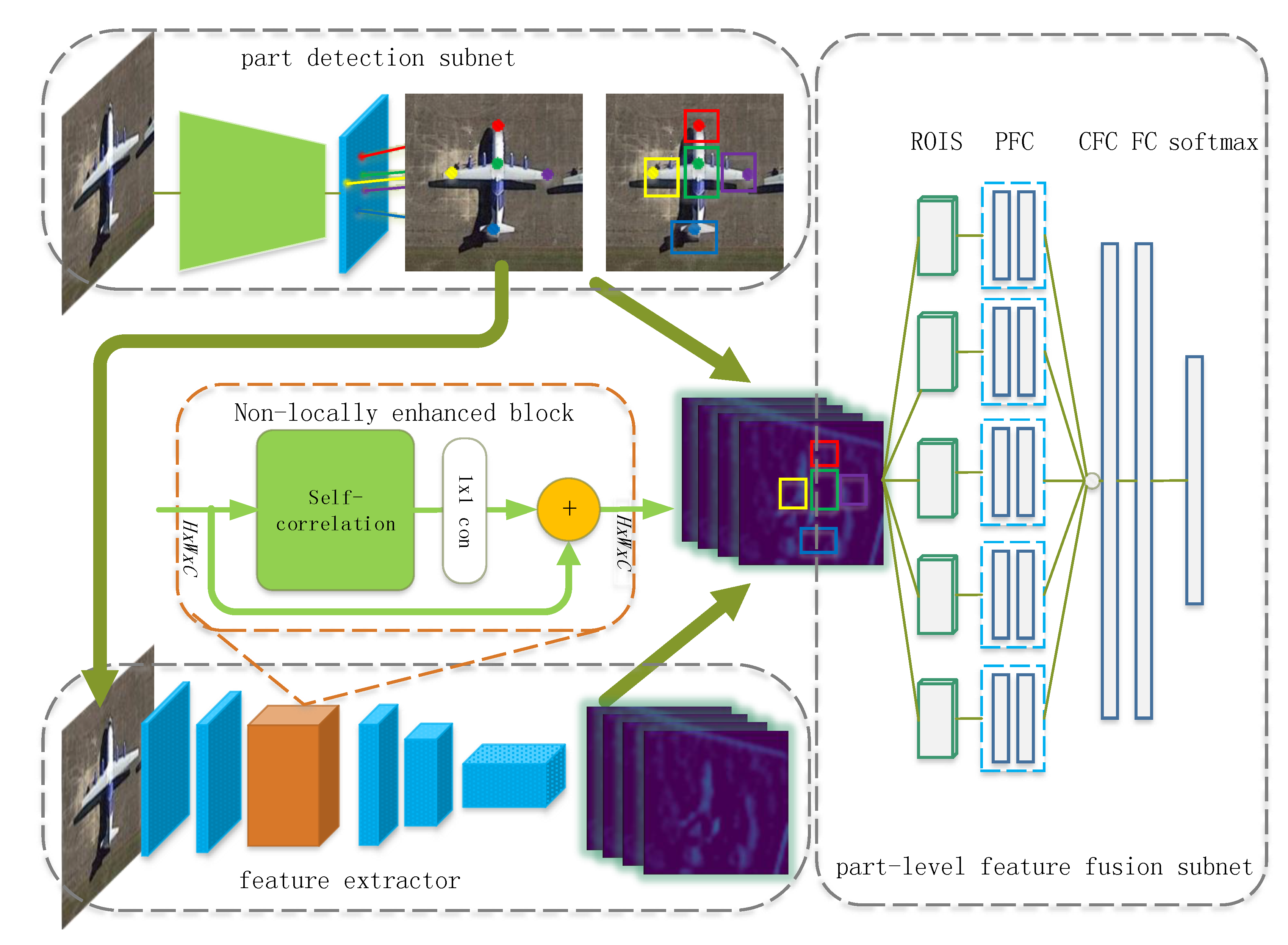
Figure 1. Framework of non-locally enhanced feature fusion network (NLFFnet).
Remotesensing 12 00681 g001
Figure 2. Aircraft examples of our dataset. The aircraft has obvious geometric features and symmetrical structure, and there are many redundant modes, which have strong long-distance correlation.
Remotesensing 12 00681 g002
Figure 3. Schematic diagram of the correlation between query and key.
Remotesensing 12 00681 g003
Figure 4. Calculation of non-locally enhanced operation.
Remotesensing 12 00681 g004
Figure 5. Decomposition of non-locally enhanced operation.
Remotesensing 12 00681 g005
Figure 6. Two ways to crop wings.
Remotesensing 12 00681 g006
Figure 7. Some hard examples in the dataset. Type-1, Type-2, Type-3, and Type-4 are four sub-categories of transport aircraft, they are very difficult to be distinguished in low-resolution remote sensing images.
Remotesensing 12 00681 g007
Figure 8. Heatmaps of aircraft Type0 before and after adding part feature fusion method. (a) original image, (b) heatmap corresponding to conv5_4 without part feature fusion, (c) the result after concatenation of the heatmap of each part, (d) the result after cutting off the heat value at the threshold, and (ei) are the heatmaps of five parts, respectively.
Remotesensing 12 00681 g008
Figure 9. Heatmaps of aircraft Type43 before and after adding part feature fusion method. (a) original image, (b) heatmap corresponding to conv5_4 without part feature fusion, (c) the result after concatenation of the heatmap of each part, (d) the result after cutting off the heat value at the threshold, and (ei) are the heatmaps of five parts, respectively.
Remotesensing 12 00681 g009
Figure 10. Heatmaps of aircraft Type41 before and after adding a non-locally enhanced module. The first row is the phenomenon without inserting the non-locally enhanced module, and the second row is the phenomenon after inserting this module, and from left to right are the original image, heatmap of conv2_2, heatmap of conv3_1 and heatmap of conv5_4, respectively.
Remotesensing 12 00681 g010
Figure 11. Heatmaps of aircraft Type40 before and after adding non-locally enhanced module. The first row is the phenomenon without inserting the non-locally enhanced module, and the second row is the phenomenon after inserting this module, and from left to right are the original image, heatmap of conv2_2, heatmap of conv3_1 and heatmap of conv5_4, respectively.
Remotesensing 12 00681 g011
Figure 12. Examples of Type1 in the training set, where (a) is obviously different from other images in that the rear side of the wing has a certain curvature, while the rear side of the wing of other images is a straight line.
Remotesensing 12 00681 g012
Figure 13. Examples of Type1 in the test set, where (a) is also different from other images in that the rear side of the wing has a certain curvature, while the rear side of the wing of other images is a straight line.
Remotesensing 12 00681 g013
Figure 14. Examples of Type27 in the training set, it can be seen that (a) in Figure 12 and Figure 13 is most likely Type27.
Remotesensing 12 00681 g014
Table 1. Comparison results of the proposed method.
MethodAccuracy
AlexNet [14]70.89%
VGG19 [15]80.39%
ResNet18 [16]79.41%
Segmentation [20]83.25%
Extractor + Non-local86.55%
Extractor + PFF87.38%
Extractor + Non-local + PFF (Proposed Method)88.56%
Table 2. Performance comparison of inserting non-locally enhanced modules at different locations of feature extractor.
LocationAccuracy
non-local module after conv1_288.17%
non-local module after conv2_2 88.56%
non-local module after conv3_4 88.36%
non-local module after conv4_4 87.34%
non-local module after conv5_4 86.78%
Table 3. Performance comparison of different loss functions.
Loss Function Accuracy
Cross-Entropy 88.56%
Focal Loss, γ =1 88.64%
Focal Loss, γ =2 88.78%
GHM-C Loss89.12%