Article

Scatter Matrix Based Domain Adaptation for Bi-Temporal Polarimetric SAR Images

1
State Key Laboratory of Information Engineering in Surveying, Mapping and Remote Sensing, Wuhan University, Wuhan 430079, China
2
School of Computer Science, Wuhan University, Wuhan 430079, China
3
Jiangsu Key Laboratory of Resources and Environmental Information Engineering, China University of Mining and Technology, Jiangsu 221116, China
4
National Remote Sensing Center of China, Ministry of Science and Technology of the People’s Republic of China, Beijing 100036, China
5
Deqing iSpatial Company, Ltd., Deqing 313200, China
6
School of Remote Sensing and Information Engineering, Wuhan University, Wuhan 430079, China
*
Author to whom correspondence should be addressed.
Remote Sens. 2020, 12(4), 658; https://doi.org/10.3390/rs12040658
Submission received: 31 December 2019 / Revised: 12 February 2020 / Accepted: 14 February 2020 / Published: 17 February 2020
(This article belongs to the Special Issue Time Series Analysis Based on SAR Images)

Abstract

:
Time series analysis (TSA) based on multi-temporal polarimetric synthetic aperture radar (PolSAR) images can deeply mine the scattering characteristics of objects in different stages and improve the interpretation effect, or help to extract the range of surface changes. However, as far as classification is concerned, it is difficult to directly generate the classification map for a new temporal image, by the use of conventional TSA or change detection methods. Once some labeled samples exist in historical temporal images, semi-supervised domain adaptation (DA) is able to use historical label information to infer the categories of pixels in the new image, which is a potential solution to the above problem. In this paper, a novel semi-supervised DA algorithm is proposed, which inherits the merits of maximum margin criterion and principal component analysis in the DA learning scenario. Using a kernel mapping function established on the statistical distribution of PolSAR data, the proposed algorithm aims to find an optimal subspace for eliminating domain influence and keeping the key information of bi-temporal images. Experiments on both UAVSAR and Radarsat-2 multi-temporal datasets show that, superior classification results with the average accuracy of about 80% can be obtained by a simple classifier trained with historical labeled samples in the learned low- dimensional subspaces.

Graphical Abstract

1. Introduction

Owing to its advantages of all-day, all-weather and multi-polarization, polarimetric synthetic aperture radar (PolSAR) has become an important part of earth observation system [1]. In recent years, it has been widely used in land cover classification [2,3,4], target detection [5], hazard assessment [6,7], surface parameter inversion [8,9] and other fields. Time series analysis (TSA) based on multi-temporal PolSAR images can deeply mine the backscattering characteristics of objects in different stages [10,11] and improve the interpretation effect [12,13,14], or help to extract the range of surface changes [15,16,17]. However, as far as classification is concerned, it is difficult to directly generate the classification map for a new temporal image, by the use of conventional TSA or change detection methods. The reasons are as follows: on the one hand, lots of the TSA research articles mainly focus on investigating the scattering behavior evolution of specific targets in different time frames, e.g., Mascolo et al. [11] and Marechal et al. [13] have successfully analyzed the seasonal impact in wetland extraction and identified crop phenological stages by using time series PolSAR images, respectively. However, the investigation on only a specific target of interest is not satisfactory in the general classification cases. On the other hand, the bi-temporal [17] and multi- temporal [18] change detection methods usually focus on distinguishing the changed and unchanged regions, or further divide the changed regions into several types of changes [16], but it is difficult to reveal the category attributes from these types, such as waterbody, buildings, grass and kinds of crops, etc. In addition, although a few classification-based change detection methods (e.g., post-classification comparison [19,20]) can generate the classification result of post-temporal image, the category-labeled samples in post-temporal image are still required in the training phase, in order to keep the high-quality interpretation.
Essentially, the problem we want to solve is how to infer the category labels of pixels in a new temporal image, by employing label information only in the historical temporal image. As implementing in-situ surveys is very time-consuming and laborious, and simultaneously the remotely sensed data volume has been growing explosively in recent years, it is certainly conceivable that the above setting will be a bottleneck to boost the classification timeliness in the near future. It seems to be simple and intuitive that we can directly train a classifier based on historical labeled samples and then employ it to classify new temporal samples. However, no matter the classification models proposed in the PolSAR field like multi-variate complex Gaussian [21] and complex Wishart classifier [22,23], or the classification models proposed in the machine learning community like support vector machine (SVM) [24], random forest (RF) [25] and deep neural network [26,27], the reliability of them is on the condition that training and test samples are independent and identically distributed (i.i.d.). Due to the high complexity of backscattering process between the transmitted microwave and ground surface, the differences of space-time attributes, incident angles and other factors, sometimes make the backscattering characteristics of similar and even identical objects very different in multiple PolSAR images. This phenomenon results in the non i.i.d. samples, and thus seriously hinders the historical category-label information to play a key role in the new temporal image classification.
As one of the research hotspots in the machine learning community, transfer learning (TL) aims at applying the previous accumulated knowledge in one field to another different but related field [28]. The field with fund of knowledge for a certain task is referred to as source domain (SD), and the field with scarce knowledge for another related task is referred to as target domain (TD). For instance, Segev et al. [29] have proposed two model TL methods based on the RF model, and combined them to deal with several cross-domain image recognition problems. The fundamental purpose of TL is to solve the problem of adapting pre-existing data to new tasks, e.g., mass of labeled email data can be used to train a good classifier for junk email recognition in SD, but only scarce labeled message data exists in TD. TL is able to improve junk message recognition precision by the use of information in SD, which provides a potential way to deal with the problem we care about. An early overview of the TL techniques can be seen in [30]. In accord with the TL terminology, hereinafter the historical temporal image and new temporal image are considered as the SD data and TD data respectively. The dual-domain data are drawn from the same feature space, and own different but related probability distributions. In the TL field, domain adaptation (DA) is a main branch which learns domain-invariant features by matching the distributions of dual-domain data. DA theory assumes via a specific mapping transformation, the samples in both domains could approximately obey the i.i.d. condition. In this case, any classifier trained with the SD samples can be directly re-used for the TD data, so employing the DA methods makes it very easy to take full advantage of the pre-existing classification models. In this respect, two regularization frameworks [31,32] proposed by Argyriou et al. can learn low-dimensional representation shared between SD and TD tasks, and Blitzer et al. [33] introduced structural correspondence learning to automatically induce correspondences among features from different domains. Moreover, dimensionality reduction and low-rank representation [34] have been applied to build DA models, such as maximum mean discrepancy embedding [35], transfer component analysis [36] and maximum independence domain adaptation [37,38] etc. The above feature-based algorithms are also collectively known as transfer subspace learning (TSL), and inspired by this, a series of deep learning models have been transplanted into the TL field recently [39,40,41,42,43]. Different from the coarse “fine-tuning” operation (i.e., start with a pretrained deep learning model and update its parameters for a new task), the models proposed in [39,40,41,42,43] involve some special designed layer modules, training strategies and so on, in order to align the joint distributions of data across domains.
In this paper, the DA theory is introduced into bi-temporal PolSAR image processing, to deal with the discrepancy of distributions between the SD and TD data. In this regard, we design a novel TSL algorithm, named scatter matrix based domain adaptation (SMbDA): firstly, it constructs two objective subfunctions to keep the category separability or unsupervised structural information in two domains, by the use of graph embedding theory and scatter matrices; later in reproducing kernel Hilbert spaces (RKHSs), the proposed algorithm employs Hilbert-Schmidt independence criterion to reduce and even remove domain influence. Furthermore, a dissimilarity measure established on the statistical distribution of PolSAR data can be used to build a specific kernel mapping function, which helps the SMbDA find a better subspace for promoting information transfer effect of bi-temporal images. Via SMbDA projection, dual-domain data approximately keeps the i.i.d. condition and valuable category information, so we can train kinds of conventional classifiers with historical labeled samples and test them with unknown samples in new temporal image.
The rest of this paper is as follows: Section 2 first gives an overview of two relevant TSL methods, and then introduces our proposed SMbDA in detail. The above methods are comparative analyzed together using UAVSAR and Radarsat-2 multi-temporal datasets. All of the experimental results and a brief discussion are respectively in Section 3 and 4. Finally, Section 5 summarizes the main content and contributions, and our future work is also presented in this part.

2. Methods

2.1. Relevant Works

Let x R D × 1 denotes the D-dimensional feature vector of a sample, the total sample set X = [ x 1   x 2   x N S + N T ] R D × ( N S + N T ) includes both the SD set X S = [ x 1   x 2   x N S ] R D × N S and the TD set X T = [ x N S + 1   x N S + 2   x N S + N T ] R D × N T , where N S and N T are the SD and TD sample sizes. If the categories of SD samples are known, then we have a SD label set C S = [ c 1   c 2   c N S ] but have no TD label set C T , here any c i { 1 , 2 , , N c } and N c is the number of categories. In general, a domain consists of two parts, its feature space and the marginal probability distribution of its dataset P ( X ) . In this paper, our focus needs to be on the marginal probability distributions of X S and X T , because time series data are drawn from the same feature space. As TSL assumes that SD and TD data would have similar low-dimensional feature structure, the discrepancy of data distributions between two domains can be reduced via mapping original data X into a new feature space, that is, the generated data Y = f ( X ) = [ y 1   y 2   y N S + N T ] R d × ( N S + N T ) , where f (     ) is a transformation function and d D .
In this subsection, two TSL algorithms are briefly reviewed and give us a few patterns to transfer information across different domains.

2.1.1. Transfer Component Analysis

Transfer component analysis (TCA) [36] is a well-known unsupervised TSL method proposed by Pan et al. in 2011. It mainly utilizes the dual-domain unlabeled data to achieve the goal of DA. In terms of image classification, the preferable adaptation effect is matching conditional probabilities, P ( C S | Y S ) P ( C T | Y T ) . Y S and Y T are respectively the generated SD and TD data using f (     ) . However, absence of C T results in the difficulty of estimating the above conditional probabilities. An alternative approach is adopted by TCA. This method try to learn f by meeting the following two conditions, and Pan et al. believe that such a f can make Y S and Y T satisfy P ( C S | Y S ) P ( C T | Y T ) .
  • Shorten the distribution distance between P ( Y S ) and P ( Y T ) as much as possible
  • Preserve the valuable information of original data X S and X T after the transformation f
For the first condition, TCA applies maximum mean discrepancy (MMD) to estimate the discrepancy of different marginal probability distributions. As a nonparametric estimation method, MMD simply calculates the distance between SD and TD sample centers in a RKHS, and does not require intermediate density estimate. For the second condition, TCA chooses to preserve data variance, and thus the principal component analysis (PCA) process is performed on dual-domain Gram kernel matrix. In addition, a regularization term used for controlling the model complexity and avoiding rank deficiency is also taken into account. In conclusion, the overall objective of TCA is minimizing both the MMD value between P ( Y S ) and P ( Y T ) , and the regularization term, with the constraint of preserving data variance.
TCA utilizes unsupervised information but ignores category labels. However, although the TD label set is scarce, it is easy to acquire the SD label set C S in many cases. Once the label information in C S is considered, a semi-supervised extension known as semi-supervised transfer component analysis (SSTCA) can be built on TCA. Besides distribution matching like the aforementioned TCA, another two conditions are also investigated in the SSTCA model:
  • Reduce the empirical error on the SD labeled data as much as possible
  • Preserve the local structure information of original data X S and X T after the transformation f
For the first condition, SSTCA applies Hilbert-Schmidt independence criterion (HSIC) to estimate the dependence between samples and the corresponding labels. Increase of the dependence is roughly equivalent to the reduction of empirical error. Similar to MMD, HSIC is a nonparametric criterion [44]. Later a detailed description about this criterion is given in Section 2.3. For the second condition, reference to manifold learning theory [45], the locality preserving projection [46] process is performed on dual-domain Gram kernel matrix. Comparatively speaking, SSTCA is much more complicated and usually performs better than TCA.

2.1.2. Maximum Independence Domain Adaptation

As a criterion for estimating the dependence between two sets, HSIC can also be used to measure the independence between data and the corresponding domain. After a DA transformation, intuitively the more independent the data is, the better the information transfer effect. A recently proposed TSL method named maximum independence domain adaptation (MIDA) [37] aims at maximizing the independence. Domain features are defined to describe the background information of samples. If only one source domain and one target domain exist, the domain feature d i of a sample x i can be expressed as the one-hot encoding form:
d i = { [ 1   0 ] T ,   i f   x i X S [ 0   1 ] T ,   i f   x i X T
So the domain feature set is D = [ d 1   d 2   d N S + N T ] , and then the dual-domain Gram kernel matrix and domain feature kernel matrix are built on dual-domain samples and set D . It is worth noting that, the samples used in MIDA are augmented with domain features, i.e., x ˜ i = [ x i T   d i T ] T . The feature augmentation operation is able to increase the initial input dimension before DA, to the benefit of better searching transformation approach. Using the above two kernel matrices, the independence (or in fact, the dependence) between dual-domain data and domain features is evaluated by HSIC. On the other hand, PCA process is also performed on Gram kernel matrix to preserve data variance. In conclusion, the objective of MIDA is simultaneously reducing domain influence (minimizing the HSIC criterion) and preserving variance (maximizing the trace of data covariance matrix).
Considering SD label information, the semi-supervised method named semi-supervised maximum independence domain adaptation (SMIDA) is built on MIDA. The idea is similar to SSTCA, videlicet, HSIC is applied again to estimate the dependence between samples and their category labels. As a result, in addition to reducing domain influence and preserving data variance, SMIDA needs to reduce the empirical error on SD labeled data.

2.2. PolSAR Data Description

In general, a PolSAR sensor alternately transmits and receives the horizontally polarized and vertically polarized electromagnetic waves. In each resolution cell, PolSAR data is represented as a 2 × 2 Sinclair matrix in brief,
S = [ S HH S HV S VH S VV ]
where all the items in Sinclair matrix are complex backscattering coefficients, and the symbol “H” indicates horizontal polarization, “V” indicates vertical polarization. Obviously, the matrix S contains abundant scattering information in different polarization state combinations, which is related to the sizes, orientations and dielectric properties of observed targets in the resolution cell.
The reciprocity principle can be satisfied in most cases, and therefore the Sinclair matrix can be equivalently vectorized as a 3 × 1 complex Lexicographic vector Ω . The superscript “T” below represents transpose operation.
Ω = [ S HH 2 S HV S VV ] T
Because distributed targets vary with time or space, and always show stochastic behaviour in SAR images, the second-order statistics of Lexicographic vector is more suitable for describing these targets than the vector itself. In practice, the covariance matrix of Ω is adopted more often:
C = Ω Ω H
The 3 × 3 Hermitian matrix C is known as polarimetric covariance matrix. Here the superscript “H” in Equation (4) denotes conjugate transpose operation, and the angle brackets denote ensemble average operation. There are totally three real-valued diagonal elements and six complex-valued off-diagonal elements in this matrix, but only nine real-valued variables are mutually independent. As vector form widely serves as the input in DA and classification algorithms, the 9 × 1 vector consisting of the nine independent real-valued variables will be used as the feature descriptor of PolSAR targets and be input into several DA and classification models in Section 3. It is worth mentioning that, an alternative input form is the magnitudes and phase angles of elements in C , however we have not observed stable and better experimental results. For simplicity, we skip the relevant content in the following part.

2.3. Scatter Matrix Based Domain Adaptation

Two DA algorithms and two semi-supervised extensions have already introduced before. It is easy to see that, TSL takes both inter-domain information influence and intra-domain information preservation into account in the DA process. SD data is able to guide TD classification, only if to some extent, the data consistency across domains and key information integrity in each domain can be guaranteed. Given historical labeled samples, our emphasis in this paper is on the post-temporal supervised classification, so the category information preservation of SD data is pivotal. However, as the semi-supervised TSL extensions, SSTCA and SMIDA both put unsupervised structural information first, and put empirical classification error reduction in second place.
Start from category information preservation, a novel semi-supervised TSL algorithm named scatter matrix based domain adaptation (SMbDA) is proposed in this subsection. During the process of eliminating domain influence, this algorithm gives priority to keeping category separability in SD, and later preserves structural information in both domains. Different from the previous TSL methods, the SMbDA prefers to investigate category distinction and thus benefits the subsequent TD classification intuitively. The objective function F of SMbDA consists of three parts:
F ( Y ) = α F S ( Y ) + β F U ( Y ) + F D A ( Y )
where F S , F U and F D A are respectively the supervised information preservation term, unsupervised information preservation term, and domain adaptation term. α and β are trade-off hyperparameters and both of them need to be nonnegative numbers. Y is the generated dataset via DA processing. As the feature descriptor of PolSAR targets is 9 × 1 vector, the feature dimension d of samples in Y is less than 9.
The integrated DA effect can be evaluated by (5). To promote nonlinear mapping ability, our SMbDA employs the similar kernel trick like TCA and MIDA. First, let a mapping function ϕ maps X into an extremely high and even infinite dimensional RKHS, leading to the implicit dataset Φ = [ ϕ ( x 1 )   ϕ ( x 2 )   ϕ ( x N S + N T ) ] , in which any ϕ ( x i ) is the feature vector of i-th sample in the RKHS. If the inner product of two RKHS vectors is represented by < ϕ ( x i ) ,   ϕ ( x j ) > , the dual-domain Gram kernel matrix K G can be defined as the equation below, where ( K G ) i j = < ϕ ( x i ) ,   ϕ ( x j ) > , N = N S + N T .
K G = [ K S S   K S T K T S   K T T ] = Φ T Φ R N × N
Equation (6) shows that, the Gram kernel matrix includes four block matrices. The diagonal ones are conventional kernel matrices built on single domain and have been widely used in kernel-based machine learning models [24]. The off-diagonal ones are cross-domain kernel matrix, and ( K S T ) i j = < ϕ ( x i ) ,   ϕ ( x N S + j ) > , ( K T S ) i j = < ϕ ( x N S + i ) ,   ϕ ( x j ) > .
In the next step, the linear dimensionality reduction is performed on Φ , or more specifically, a projection matrix U ϕ is used to transform Φ into the desired dataset Y R d × N , and Y = U ϕ T Φ . Because each projection direction can be expressed as a linear combination of all samples in the RKHS [35,36,37], we have U ϕ = Φ U , U R N × d , and thus Y = U T Φ T Φ = U T K G . Obviously, it does not matter that the explicit form of function ϕ is undefined, as Y is just related to the Gram kernel matrix and projection matrix. Once the inner product operation, also known as kernel mapping function, is selected, the matrix K G is determinate. As a consequence, Y changes only when U changes, and hence (5) can be rewritten as:
F ( U ) = α F S ( U ) + β F U ( U ) + F D A ( U )
The optimal U can be obtained by maximizing (7), and later Y is generated based on U . When an out-of-sample x comes, the inner product of ϕ ( x ) and each ϕ ( x i ) in Φ should be calculated at first, and later the corresponding projection vector of x would be gotten, using the product result of the previous step and projection matrix U .
In order to avoid trivial solutions, some specific constraints need to be added, e.g., orthogonal constraint U T U = I d , I d is a d × d identity matrix. From the above, the objective of SMbDA is (8). The remainder of this subsection will describe the main components F S , F U and F D A in detail.
U = arg max F ( U ) ,   s . t .   U T U = I d

2.3.1. Supervised Information Preservation

The difficulty level of object identification depends on category separability, that is, decided by both inter-category scatter and intra-category scatter. Linear discriminant analysis (LDA) [47] maximizes the former and minimizes the latter using a trace ratio operation. Instead of trace ratio, maximum margin criterion (MMC) [48] is inspired by the well-known SVM classifier and adopts a trace difference operation to achieve the similar goal. In comparison to LDA, MMC avoids the rank defect problem and therefore improves the robustness of solutions. Here we introduce and further generalize this criterion to the DA scope.
Consistent with the previous works, the SD sample set X S , SD label set C S and TD sample set X T are given, but there is no TD label set in our semi-supervised setting. Denote the separability between the i-th and j-th categories as J i j , then the total category separability J is a weighted sum:
J = 1 2 i = 1 N c j = 1 N c P i P j J i j
P i and P j are the prior probabilities of the i-th and j-th categories. Because the prior distributions of categories are all unknown, these probabilities are assumed to be equivalent, so P i = P j = 1 / N c . The factor “1/2” in Equation (9) is for balancing the total separability, as separability is symmetric, e.g., J i j = J j i . J is an indicator to judge whether the labeled samples are easy to classify. In other words, it is able to evaluate the effectiveness of supervised information in a certain feature space.
The separability J i j needs to comprehensively investigate inter- and intra-category dispersions. As for the generated SD sample set Y S = [ y 1   y 2   y N S ] , MMC represents inter-category dispersion as the square of distance among category centers, and represents intra-category dispersion as the trace of intra-category scatter matrix, so
J i j = y ¯ S i y ¯ S j 2 S c i S c j
where,
S c i = T r ( m = 1 n i ( y m i y ¯ S i ) ( y m i y ¯ S i ) T )
S c i and y ¯ S i are respectively the dispersion and center of i-th category, so do S c j and y ¯ S j . The m-th sample in i-th category is y m i , and n i is the sample size of i-th category.     denotes l 2 norm, T r (     ) is trace operator. Substitute (10) into (9), and we get
J = 1 2 i = 1 N c j = 1 N c P i P j y ¯ S i y ¯ S j 2 1 2 i = 1 N c j = 1 N c P i P j ( S c i + S c j )
The square of distance can be expanded to,
y ¯ S i y ¯ S j 2 = T r ( ( y ¯ S i y ¯ S j ) ( y ¯ S i y ¯ S j ) T ) = T r ( ( y ¯ S i y ¯ S ) ( y ¯ S i y ¯ S ) T + ( y ¯ S y ¯ S j ) ( y ¯ S y ¯ S j ) T + ( y ¯ S i y ¯ S ) ( y ¯ S y ¯ S j ) T + ( y ¯ S y ¯ S j ) ( y ¯ S i y ¯ S ) T )
where y ¯ S is the sample center of Y S , hence i = 1 N c P i ( y ¯ S y ¯ S i ) = 0 . After derivation, it is shown that,
1 2 i = 1 N c j = 1 N c P i P j ( ( y ¯ S i y ¯ S ) ( y ¯ S y ¯ S j ) T + ( y ¯ S y ¯ S j ) ( y ¯ S i y ¯ S ) T ) = 0
Using (13) and (14), the first term in (12) can be derived as,
1 2 i = 1 N c j = 1 N c P i P j y ¯ S i y ¯ S j 2 = i = 1 N c j = 1 N c P i P j T r ( ( y ¯ S i y ¯ S ) ( y ¯ S i y ¯ S ) T ) = 1 N c T r ( i = 1 N c ( y ¯ S i y ¯ S ) ( y ¯ S i y ¯ S ) T )
which is basically consistent with the total inter-category scatter in LDA. Based on graph embedding [49], we can directly use the matrix description Y S S B Y S T instead of the expression i = 1 N c ( y ¯ S i y ¯ S ) ( y ¯ S i y ¯ S ) T in Equation (15), and S B = i = 1 N c e S i ( e S i ) T / n i e S e S T / N S . e S is a N S × 1 vector and its elements are all one. e S i is also a N S × 1 vector with ( e S i ) j = 1 if the label c j of j-th SD sample is i ; 0 otherwise.
On the other hand, the second term in (12) can be expanded to Equation (16), which is basically consistent with the total intra-category scatter in LDA. Similar to (15), the matrix description Y S S W Y S T can be used instead of i = 1 N c m = 1 n i ( y m i y ¯ S i ) ( y m i y ¯ S i ) T , and S W = I N S i = 1 N c e S i ( e S i ) T / n i .
1 2 i = 1 N c j = 1 N c P i P j ( S c i + S c j ) = 1 N c i = 1 N c S c i = 1 N c T r ( i = 1 N c m = 1 n i ( y m i y ¯ S i ) ( y m i y ¯ S i ) T )
Taken (15) and (16) into account, the total category separability is,
J = 1 N c T r ( Y S S B Y S T ) 1 N c T r ( Y S S W Y S T )
The capacity of supervised information preservation of Y S can be evaluated by J . Besides, the connection between Y and J should be built in the DA learning scenario. We put Y into (17), and accordingly adopt two generalized matrices S ^ B and S ^ W instead of S B and S W . Finally, we obtain the first subfunction F S of SMbDA based on MMC.
F S ( U ) = T r ( Y S ^ B Y T ) T r ( Y S ^ W Y T ) = T r ( U T K G ( S ^ B S ^ W ) K G U )
and,
S ^ B = [ S B O N S × N T O N T × N S O N T × N T ]
S ^ W = [ S W O N S × N T O N T × N S O N T × N T ]
O represents a matrix with all zero elements. Compared with (17), the scaling constant 1 / N c is omitted in (18). It is easy to see that, J and F S are equivalent, except the difference of input modes.

2.3.2. Unsupervised Information Preservation

Learning the projection matrix U by only preserving category separability is not enough. If the fundamental structural information of dual-domain samples is distorted after projection, the difficulty of subsequent classification is inevitable. However in most cases, only SD samples are labeled, so unsupervised information preservation is also necessary. Considering the high simplicity and practicability of PCA, the proposed SMbDA aims at maximizing data variance. As Y = U T K G , the variance of Y is,
V a r ( Y ) = i = 1 N y i y ¯ 2 = T r ( i = 1 N ( y i y ¯ ) ( y i y ¯ ) T ) = T r ( U T K G H K G U )
in which, y ¯ represents the sample center of Y , and H = I N e e T / N is the centering matrix. e is a N × 1 column vector and all the elements are one. We can further simplify (21) by normalizing Gram kernel matrix. Namely, normalize K G as K G e e T K G / N K G e e T / N e e T K G e e T / N 2 beforehand, and hence H can be deleted. In this case, the second subfunction of SMbDA, F U ( U ) = T r ( U T K G K G U ) , is obtained.

2.3.3. Domain Influence Reduction

Except investigating supervised and unsupervised information of dual-domain data, domain influence ought to be reduced. As previously mentioned in Section 1, one of the most important goals in the DA field is to approximately hold the i.i.d. condition. That is to say, via the projection in RKHSs, it should look like that the SD and TD data are drawn from the same distribution. But this requirement is always hindered by inter-domain variable factors. Therefore, we consider to achieve this goal by virtue of reducing the dependency between data and domains. If the projected data Y are independent of the relevant domains, the domain which any sample in Y belongs to cannot be distinguished, and thus in the specific feature space, the inter-domain discrepancy is diminished.
As HSIC is a simple and nonparametric approach to estimate the dependency between two sets, we employ it to measure the dependency between Y and domain features. Similar to MIDA, domain features are defined as the one-hot encoding form [37] and are used to describe the background information of samples. When there are only one SD and one TD, the domain feature d i of a sample x i is shown in Equation (1), and the domain feature set D = [ d 1   d 2   d N S + N T ] is built. Because HSIC calculates the square of the Hilbert-Schmidt norm of the cross-covariance operator, an empirical estimation form of HSIC is represented as [50],
H S I C ( A , B ) = 1 ( n 1 ) 2 T r ( H K A H K B )
where A and B are the sets we want to measure the dependency, K A and K B are respectively the kernel matrices of the two sets, n is the number of samples in sets. A small HSIC value implies a weak dependence between A and B . Only if A and B are independent, HSIC reaches the minimum value, zero.
Substituting the kernel matrices of Y and D into (22), the dependency between data and the corresponding domains is evaluated. The kernel matrices K Y of Y is Y T Y = K G U U T K G , and using the linear kernel function, the kernel matrix K D of D is D T D . For convenience, if K G is normalized in advance, we can also omit the centering matrix H and the scaling factor in (22). As a consequence, the last subfunction F D A of SMbDA can be written as:
F D A ( U ) = H S I C ( Y , D ) = T r ( K G U U T K G K D ) = T r ( U T K G K D K G U )
From all the above, our SMbDA aims at maximizing the category separability, data variance, and simultaneously minimizing domain dependence by a linear projection in the RKHS. Combining three equations (18), (21) and (23), the overall objective of SMbDA is
U = arg max F ( U ) = arg max T r ( U T K G ( K D + α S ^ B α S ^ W + β I N ) K G U ) s . t .   U T U = I d
Solving (24) is equivalent to find the eigenvectors of K G ( K D + α S ^ B α S ^ W + β I N ) K G . The eigenvectors corresponding to the d largest eigenvalues are the column vectors in U .

2.4. Wishart-Based Radial Basis Function

The selection of kernel mapping function is of great importance on the algorithm performance. Gaussian radial basis function (RBF) is a widely-used kernel function in image processing, which is defined as,
R B F G ( a , b ) = exp ( a b 2 2 σ 2 )
b where a ,are two arbitrary real-valued vectors. σ is a smoothing parameter and should be a positive number.
This function is the exponent of negative weighted square of the distance between feature vectors. It is evident that, a suitable distance measure is to the benefit of promoting the potential of RBF. In our previous work [1], a Wishart distribution-derived dissimilarity measure has been used to build a simple classification model, which achieves better experimental results than the classical Wishart classifier [22] and several mainstream models. We believe that, this measure is helpful to build a new RBF that is more suitable for PolSAR data. This dissimilarity measure is defined as,
d m ( C 1 , C 2 ) = 2 log | C ¯ | log | C 1 | log | C 2 |
C 1 , C 2 are the polarimetric covariance matrices of samples, and C ¯ = ( C 1 + C 2 ) / 2 , | | means the determinant operation. Note that, (26) is available for multi-look PolSAR data.
Because the square root of d m meets the nonnegativity, definiteness, symmetry and triangle inequality properties, d m can be called as metric. Replace a b with d m , the new kernel function is
R B F W ( C 1 , C 2 ) = exp ( 2 log | C ¯ | + log | C 1 | + log | C 2 | 2 σ 2 )
The symmetry property of d m indicates that, R B F W is a positive semi-definite function, so R B F W meets Mercer kernel theorem. As d m is derived from Wishart distribution, R B F W is named as Wishart-based RBF hereinafter.
In general, the SMbDA Algorithm 1 is easy to implement and can be summarized as follows.
Algorithm 1. SMbDA
Input: SD and TD sample sets X S , X T , and SD label set C S
Output: projection matrix U
Step 1. Define domain feature of each sample based on (1) and form domain feature matrix D
Step 2. Construct Gram kernel matrix K G based on (6) (Wishart-based RBF is recommended)
Step 3. Normalize K G as K G e e T K G / N K G e e T / N e e T K G e e T / N 2
Step 4. Construct two scatter-related matrices S ^ B and S ^ W based on (19) and (20)
Step 5. Calculate the kernel matrix K D of domain features, K D = D T D
Step 6. Eigen decompose the matrix K G ( K D + α S ^ B α S ^ W + β I N ) K G
Step 7. Select the d leading eigenvectors to construct the projection matrix U

2.5. Relationship with Other Methods

Leaving the difference of kernel mapping functions alone, the proposed SMbDA algorithm is closely related to a series of dimensionality reduction and TSL methods:
  • If the SD and TD data are regarded as a whole without considering inter-domain discrepancy, the Gram kernel matrix K G degrades into traditional kernel matrix, and accordingly the unsupervised information preservation term degrades into the objective function of standard PCA in kernel spaces. Then if we set α = 0 , SMbDA is the same as kernel PCA.
  • If we only pay attention to SD samples, SMbDA is further simplified down to a kernel-based combination of MMC and PCA, which can be seen as a semi-supervised dimensionality reduction algorithm. We use two core matrices S B and S W to capture scatter information and preserve category separability. Originally, the two matrices were used in LDA and kernel LDA. In this paper, they are generalized and reused for dual-domain kernel matrix. In source domain, our SMbDA is similar to the idea in [51], in which a combination of local LDA and PCA was discussed.
  • As the inter- and intra-category scatter matrices have been reformed in [49], the proposed algorithm has an implicit relationship with the graph embedding framework. From this perspective, the term K D + α S ^ B α S ^ W + β I N can be regarded as a special Laplacian matrix.
  • SMbDA, TCA and MIDA have some points in common. All of the three algorithms use the covariance matrix of data to keep unsupervised information, and try to reduce the negative cross-domain influence. However, TCA, MIDA and their semi-supervised extensions primarily consider unsupervised information. On the contrary, SMbDA primarily makes full use of label information to keep category separability, which makes it more benefit for classification in theory. Besides, SMbDA avoids inversion operation when solving projection matrix, and thus is more efficient than TCA and SSTCA.

3. Materials and Results

3.1. Experimental Datasets and Parameter Settings

As in practice, TD samples are usually unlabeled, it is very difficult to transfer valuable information from SD to TD. Therefore, two groups of experiments have been conducted in this section. The first group is based on a multi-temporal PolSAR dataset obtained by the airborne UAVSAR system in Winnipeg, Canada. The time intervals are only several days, so the difficulty of DA and classification is relatively low. The second group is based on another multi-temporal PolSAR dataset obtained by the Radarsat-2 satellite in Erguna, China. The time intervals are as long as several months and the spatial distribution of objects was very different in time frames, so this group is much closer to reality.
In both groups, discriminant analysis classifier (DAC) was selected as our classification model, and we investigated the classification performances when applying different DA algorithms, including TCA, SSTCA, MIDA, SMIDA and SMbDA. On one hand, Gaussian RBF was used for all the five algorithms to compare the effectiveness of them; on the other hand, Wishart-based RBF was also used for SMbDA to compare the effectiveness of different RBFs. The SMbDA model with Wishart-based RBF is called as WSMbDA for short. Our goal is to use the classifier trained with historical labeled samples to classify the samples in a new temporal image. So in the training phase, the samples in X S and X T have been picked randomly, and only the labels of SD samples were given to the DAC and DA methods. In the test phase, lots of TD out-of-samples were projected into the learned subspaces and then classified. The sample selection, domain adaptation and classification steps have been repeated 10 times to obtain reliable performances.
Before the training phase, we picked some labeled TD samples to compare the classification results under different hyperparameter values and projection dimensions, and finally decided the optimal parameters for subsequent experiments. In our experiments, the search strategy refers to [36,37]. For the proposed SMbDA and WSMbDA, we first fixed α = 1 ,   β = 1 e 4 and searched for the best σ value in [ 10 6 ,   10 ] . Afterwards, we fixed σ and searched for the best α value in [ 0 ,   10 ] . Finally, both σ and α were fixed and we searched for the best β value in [ 0 ,   10 ] . The big difference between the initial values of α and β is because the assumption that in a cross-domain classification task, supervised information is more likely to be helpful than unsupervised information. As the ranges of hyperparameters were continuous, logarithmic sampling was implemented. The same strategies were applied to TCA, SSTCA, MIDA and SMIDA, in order to fairly evaluate and compare these algorithms.

3.2. Experiments on UAVSAR Dataset

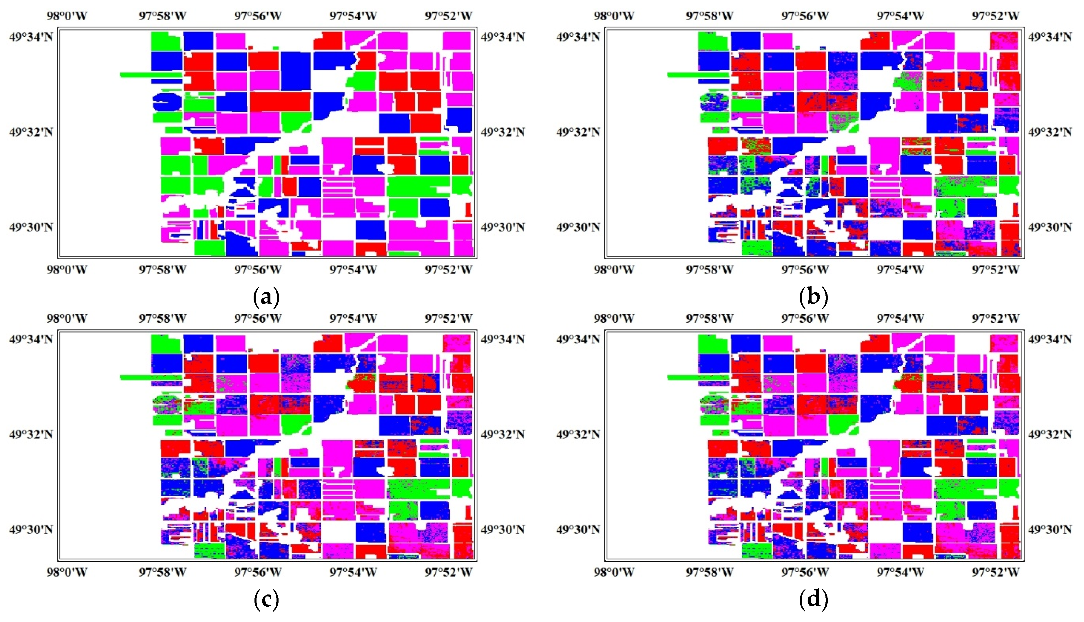
The UAVSAR dataset includes three PolSAR images. The acquisition times are 2012-07-05, 2012-07-08 and 2012-07-17, respectively recorded as Domain A, Domain B, Domain C in this subsection. After 4 × 4 multi-look preprocessing and geocoding, the image sizes are all 295 × 413 pixels. The PauliRGB images are shown in Figure 1. Pairing the three domains, there are totally six DA and classification tasks: A->B, B->A, A->C, C->A, B->C, C->B. 100 samples per category were randomly selected in the training phase.
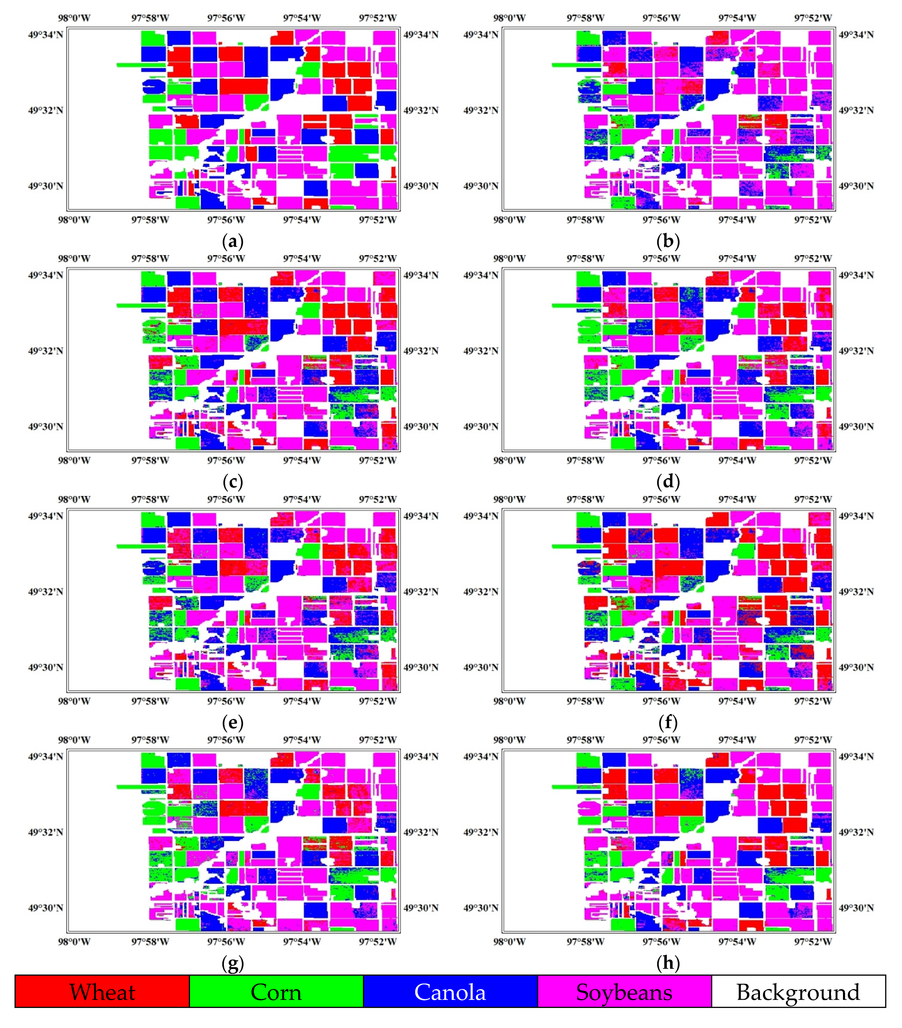
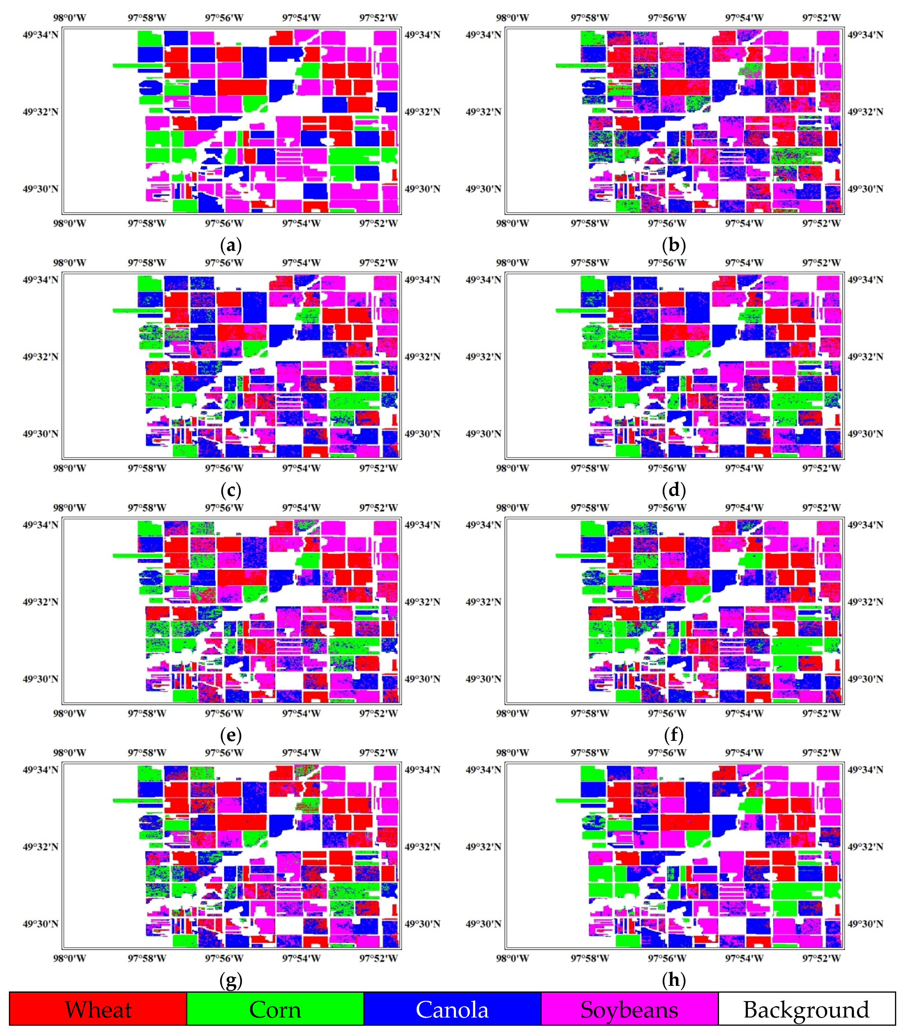
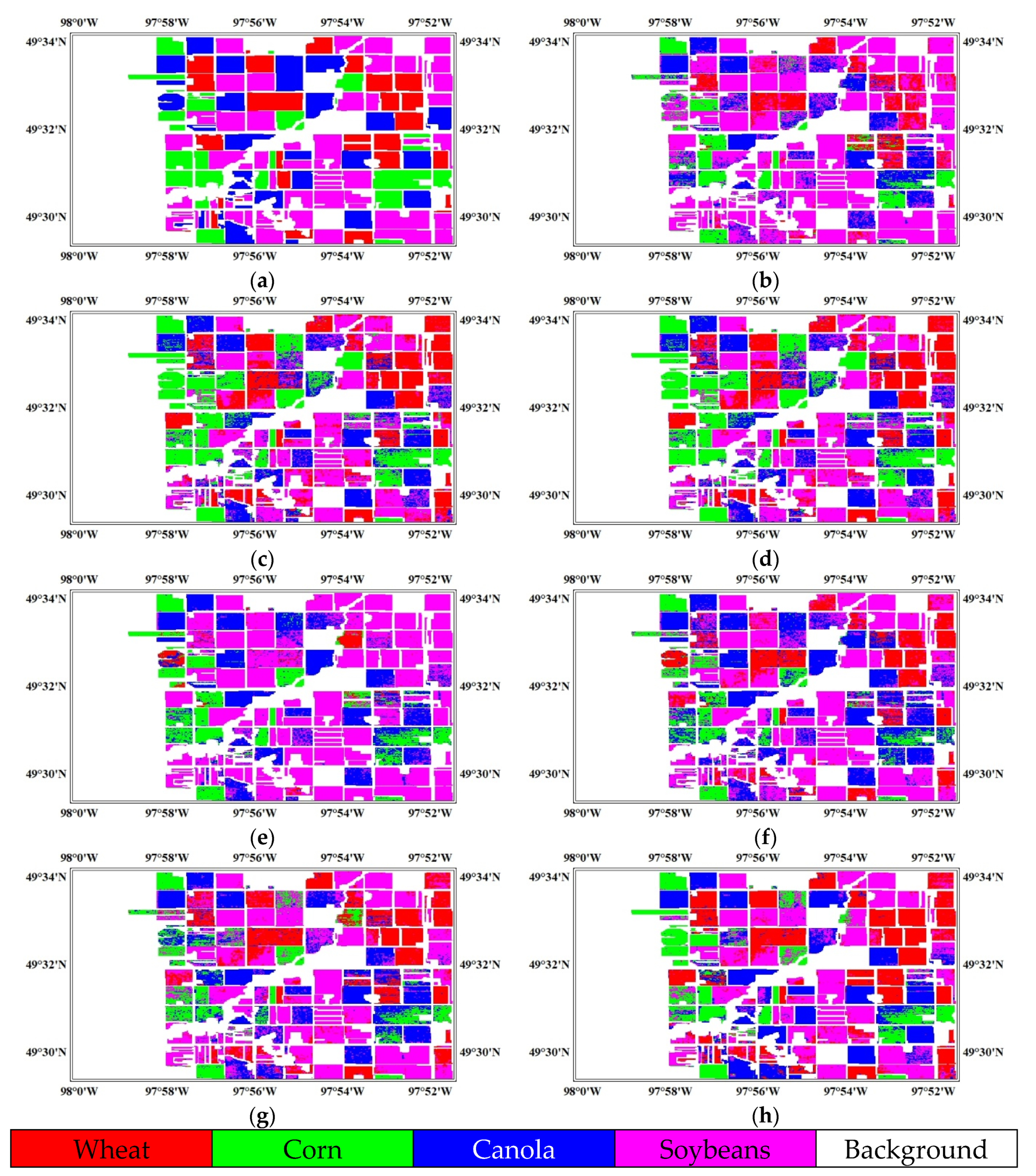
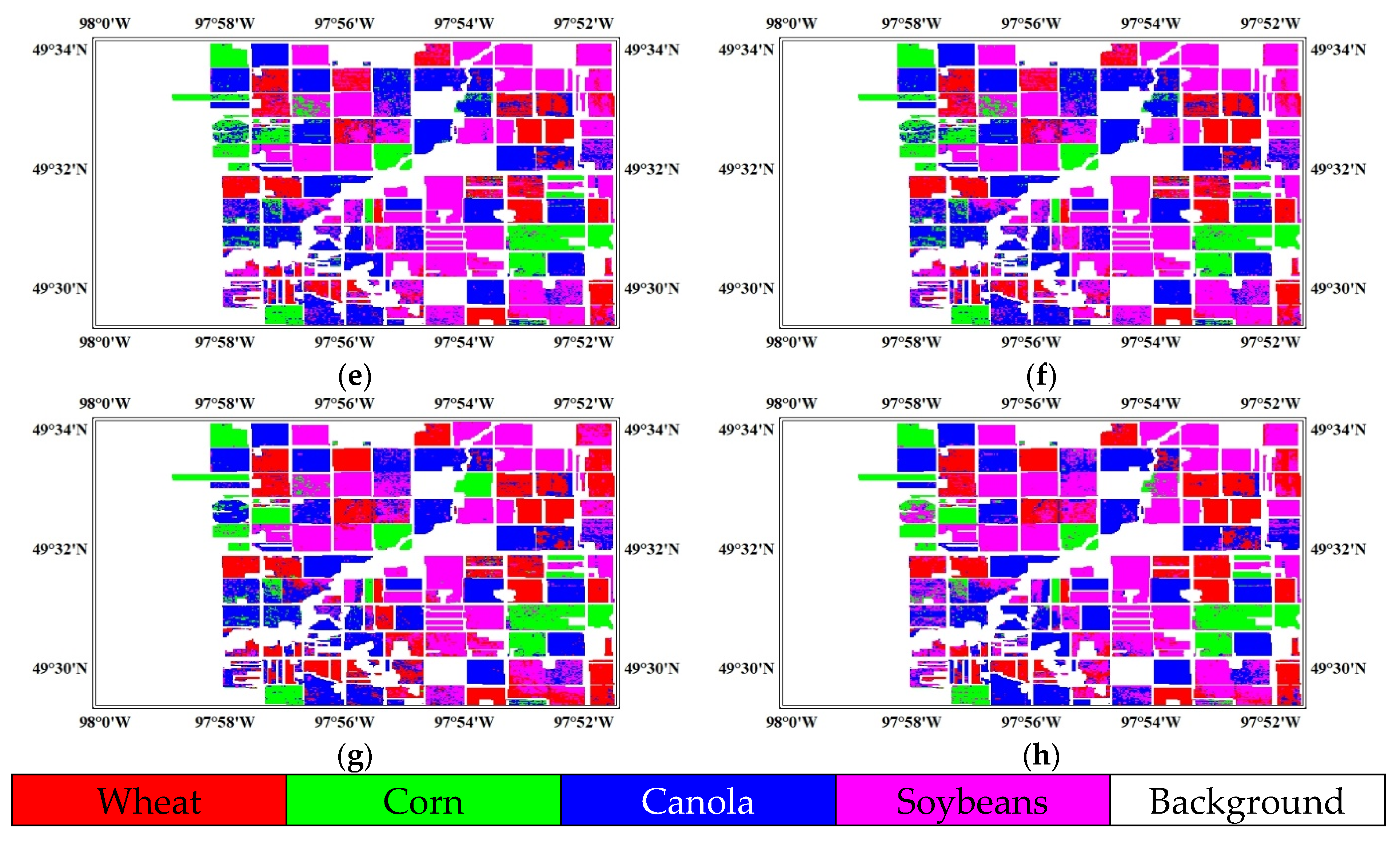
Because the time intervals are very short, the categories of objects in the three images have not changed, so the correlation between any two images is very strong, and the difficulty of DA is relatively low. Although it seems that DA has no practical application significance for this dataset, it can still help us test DA effects under ideal conditions. Moreover, since most of the crops in this area were in their growing stage, there are indeed some backscattering differences of the same category in different times. The classification maps are generated by the use of different methods, as shown in Figure 2, Figure 3, Figure 4, Figure 5, Figure 6 and Figure 7.
By comparing the classification maps with ground truth map, it is found that the overall DA effects between Domain A and Domain B are significantly better than that between Domain A and Domain C, Domain B and Domain C. The reason is that, the data distribution discrepancy between Domain A and Domain B is very small (time interval is just 3 days), but the discrepancies between Domain A and Domain C, Domain B and Domain C are larger (time intervals are 12 days and 9 days). Furthermore, by observing the DA effect between Domain A and Domain C, and the DA effect between Domain B and Domain C, we find the latter is better than the former, because the imaging time between Domain B and Domain C is closer. This point also proves that inter-domain correlation can directly affect the difficulty level of DA, which is consistent with our intuition.

3.3. Experiments on Radarsat-2 Dataset

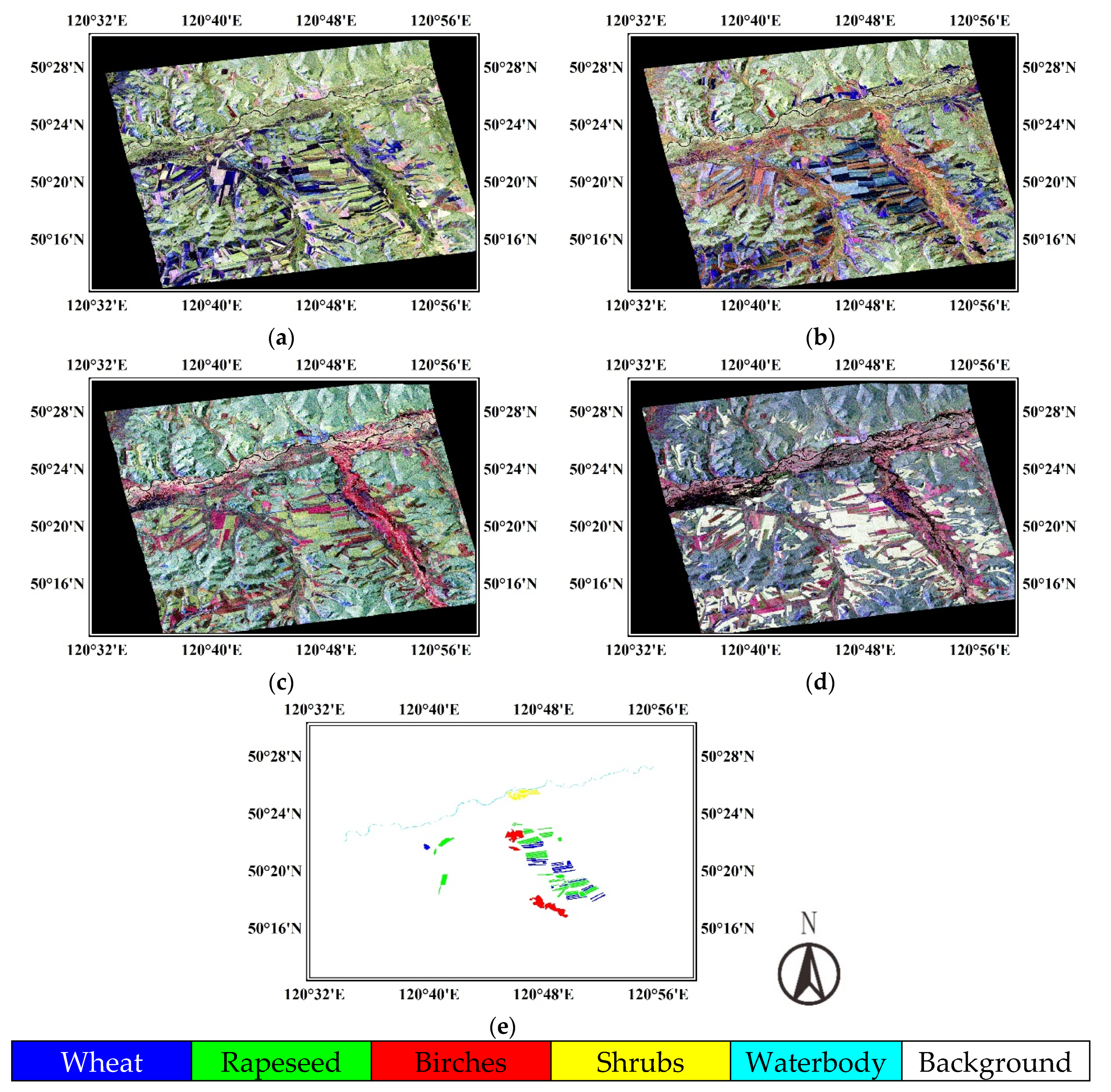
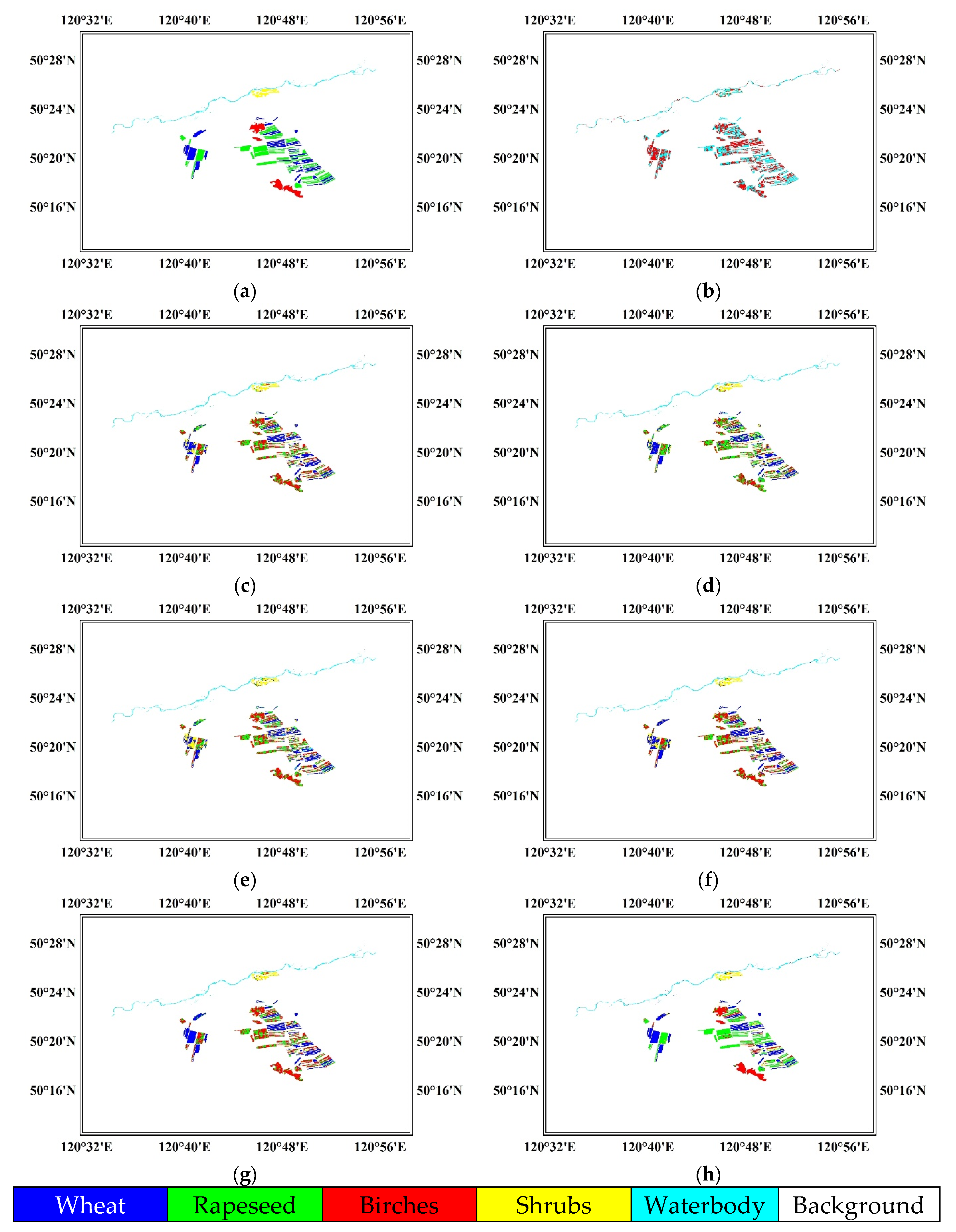
The Radarsat-2 dataset includes four PolSAR images. The acquisition times are 2012-09-01, 2013-06-16, 2013-07-10 and 2013-08-03, respectively recorded as Domain A, Domain B, Domain C and Domain D in this subsection. A 4 × 4 multi-look operation has been carried out to suppress speckle noises and reduce image sizes. After geocoding, the sizes are all 1091 × 1274 pixels. Four PauliRGB images are shown in Figure 8a–d, and the corresponding ground truth maps are displayed in Figure 8e, Figure 9a, Figure 10a, Figure 11a. There are five main types of ground objects in the imaging area: wheat, rapeseed, birches, shrubs and waterbody. As two kinds of crops, wheat and rapeseed both own different scattering characteristics in different growth stages. Birches and shrubs are also able to vary with seasons, local incidence angles and other factors. All these conditions have a bad impact on cross-domain learning. Moreover, the spatial distribution of crops has also changed from 2012 to 2013. Therefore, this dataset can be used as a typical verification data to test the performance of DA algorithms.
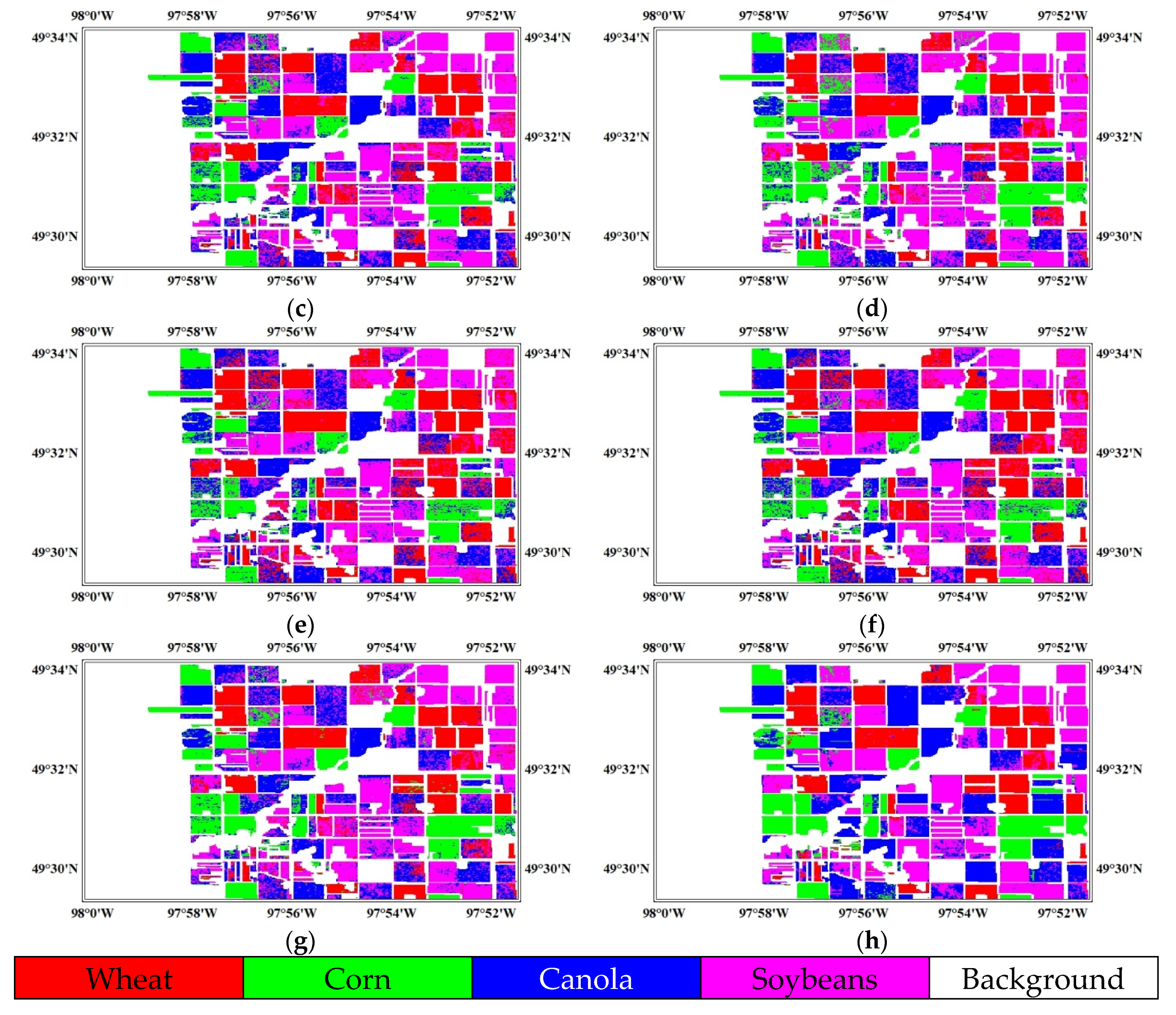
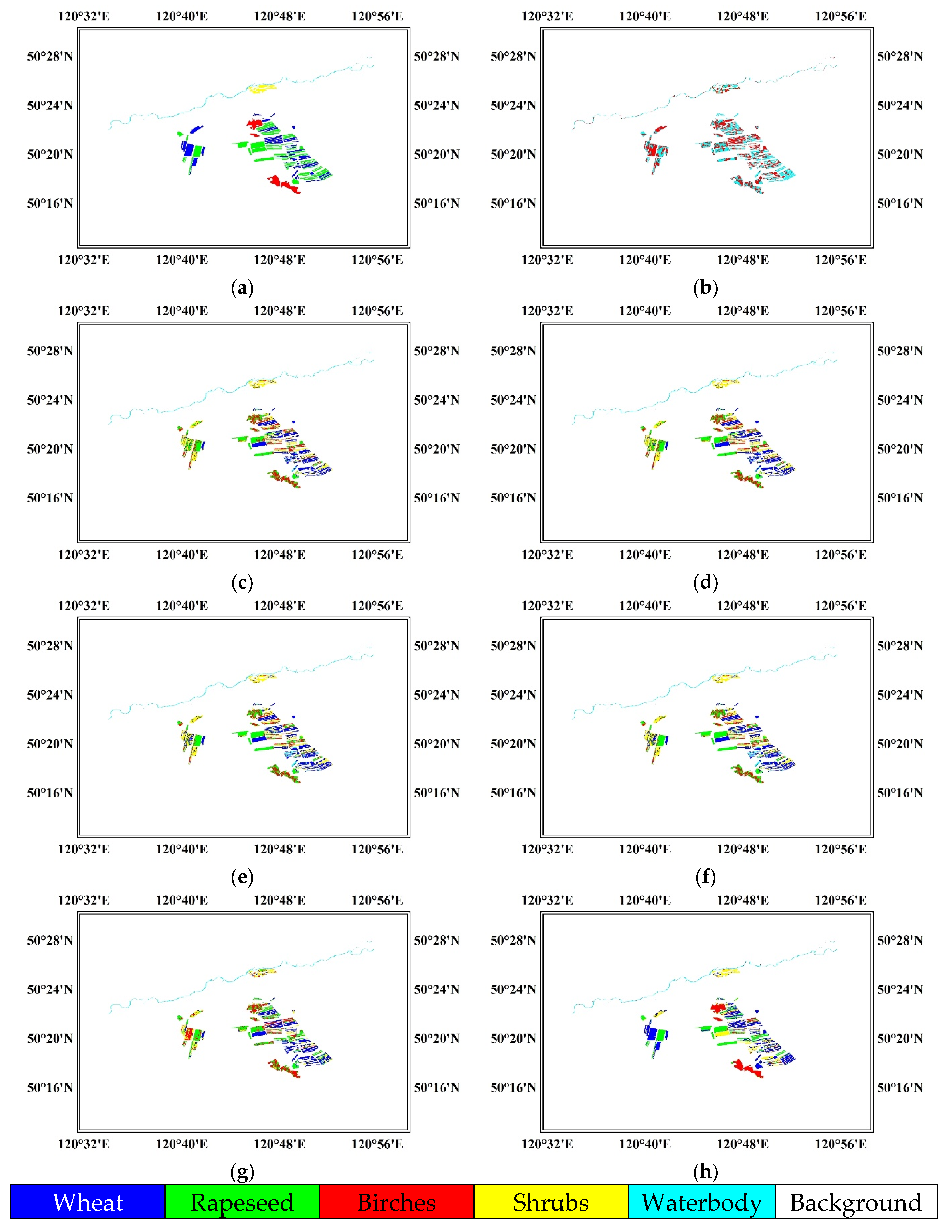
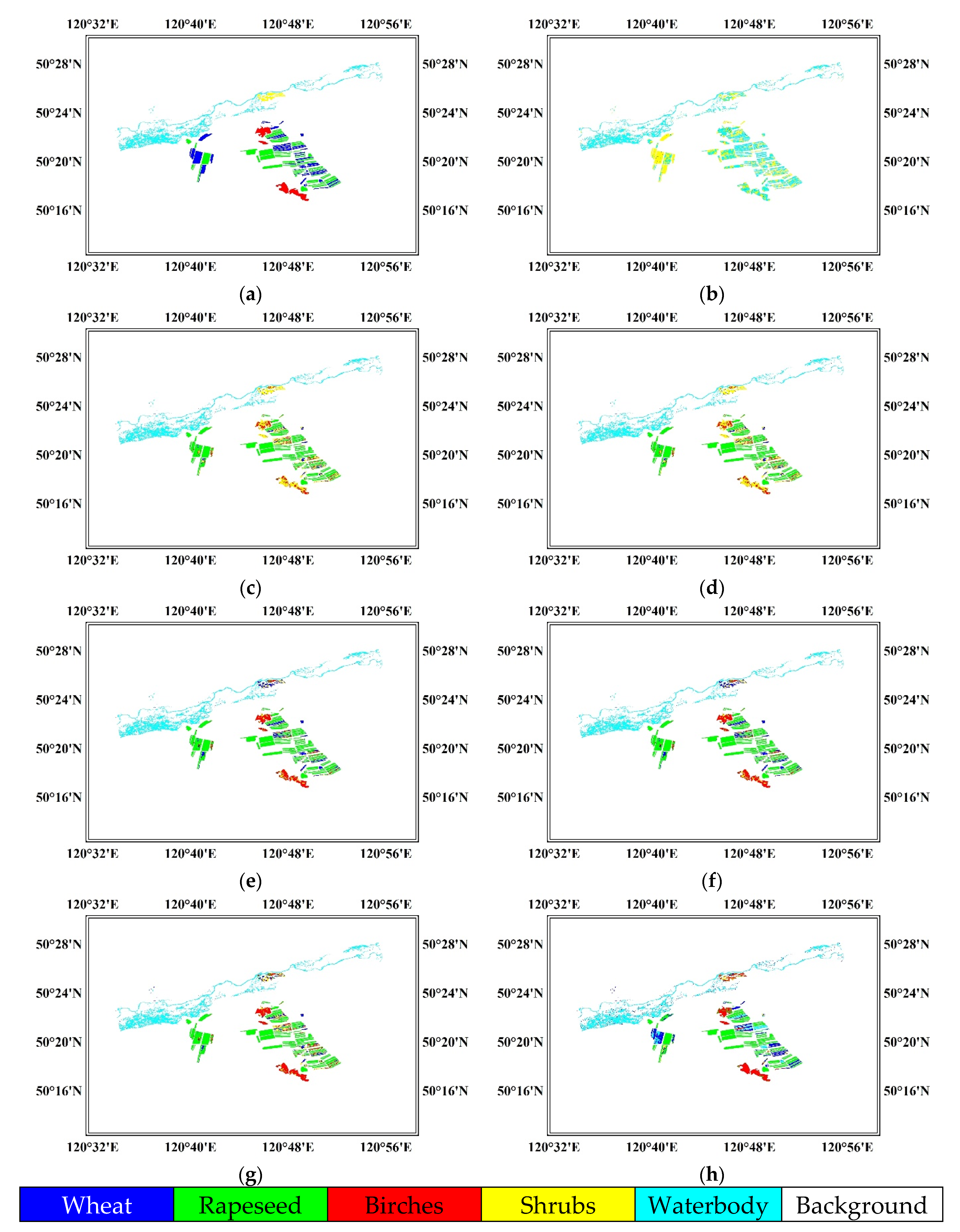
In this subsection, we have conducted three challenging tasks: A->B, A->C, A->D, i.e., only use the labeled samples acquired on 2012 to classify the unlabeled samples acquired on 2013. 200 samples per category were randomly selected in the training phase. The classification maps are generated by the use of different methods, as shown in Figure 9, Figure 10 and Figure 11. Obviously, the three tasks are much more difficult than those in the previous subsection. Because the time intervals are less than two weeks in the UAVSAR dataset, the distribution discrepancies of this dataset are not very large. Even if we skip the DA step and directly use DAC to classify TD samples, the classification maps shown in Figure 2, Figure 3, Figure 4, Figure 5, Figure 6 and Figure 7b are still acceptable in part. But without any DA processing, the classification maps generated directly by DAC in Figure 9, Figure 10 and Figure 11b are almost completely wrong. Fortunately, all the DA methods take inter-domain distribution into account. As a result, the classification results shown in Figure 9, Figure 10 and Figure 11c–h have significant improvements in different degrees. Besides, the performance of direct classification in the last task is significantly better than the first two, and a similar tendency happens in other methods as well. The reason is that, the backscattering information of same categories can be relatively similar in adjacent months. The imaging times in the last task satisfies this condition (Domain A: September, Domain D: August).

4. Discussion

In this part, two quantitative indices, overall accuracy (OA) and Kappa coefficient (Kappa), are selected to evaluate the performances of different DA algorithms. The precision evaluation results of two experiments are listed in Table 1 and Table 2. The results given in Table 1 are consistent with our findings in Section 3, and it is obvious that four conclusions can be drawn from the table:
  • No matter in which task, the OA and Kappa values are generally upgraded after DA processing. It is proved that DA is of significant help for these classification tasks, especially the three tasks, Domain B -> Domain A, Domain A -> Domain C and Domain B -> Domain C.
  • Compared with TCA and MIDA, SSTCA and SMIDA are more conducive to improving interpretation performances, as both of them take label information into account. Even in the worst case, the two can be respectively equivalent to TCA and MIDA.
  • In all of the tasks, our proposed SMbDA caused no negative transfer effect, and has achieved better performances than TCA, SSCTA, MIDA and SMIDA in half of the tasks. In the other half, the OA and Kappa values of SMbDA are basically close to the best ones.
  • WSMbDA can further improve the performances of SMbDA in most cases, and has obtained the best results in general, which verifies the superiority of Wishart-based RBF. The well-designed DA model SMbDA, coupled with the suitable kernel mapping function, is able to achieve the average OA value of more than 80% and the average Kappa value of more than 0.75.
Similar to the precision evaluation results in Winnipeg, SMbDA has generally achieved better performances than TCA, SSTCA, MIDA and SMIDA in Erguna, while WSMbDA has shown great advantages with the highest OA of 84.1% and Kappa of 0.775 in Table 2. An interesting phenomenon is that, although the two evaluation indices of each method (except DAC) in the last task are very high, a large proportion of wheat was mistakenly classified into the rapeseed category in Figure 11c–g, resulting in the disappearance of blue areas in these classification maps. In contrast, although the overall performances of most of DA methods are poor in the first two tasks, the blue areas of wheat still exist in Figure 9 and Figure 10. This is because the two kinds of crops are both mature in the third task and thus the volume scattering components of them are both large, which causes the confusion between wheat and rapeseed. In addition, the wavelength of C-band microwave used by Radarsat-2 is short and accordingly the penetrability is weak. This point further aggravates the above dilemma. As a consequence, most of DA methods failed to preserve the backscattering differences between the two crops. This situation would change with longer wavelength. As seen from Table 2, the direct DAC classification results are very bad, the OA values are only 11%-20% and the Kappa values are around zero. However, WSMbDA always performs well. Especially in the task Domain A -> Domain D, WSMbDA is still able to accurately distinguish the main categories.

5. Conclusions

With the rapid growth of remotely sensed data volume, the inefficient in-situ surveys will limit classification timeliness in the near future. Domain adaptation helps to adapt pre-existing data to new tasks, which provides a potential way to deal with this problem. In this paper, a novel semi-supervised domain adaptation algorithm, named scatter matrix based domain adaptation, has been proposed to transfer and share valuable information between bi-temporal PolSAR images. Different from the previous methods, the proposed algorithm pays more attention to supervised information preservation and hence is very helpful for supervised classification task. Empirical results have demonstrated that after applying it, the superior post-temporal classification maps can be obtained by a simple classifier trained with labeled samples in pre-temporal PolSAR imagery. Moreover, the performance of this algorithm can be further improved by the use of Wishart-based kernel mapping function. Apart from time series image processing, we believe the proposed algorithm also has the potential to adapt cross-regional PolSAR images. However, how to determine the hyperparameter values is still an opening issue. We plan to design an adaptive hyperparameter selection strategy in the future. Besides, this paper mainly focuses on the situation of single pre-existing source domain. We would like to generalize the proposed algorithm and make it suitable for multiple domains.

Author Contributions

Conceptualization, W.S.; Investigation, L.T.; Methodology, W.S.; Supervision, P.L., B.D., J.Y. and L.Z.; Validation, M.L. and L.Z.; Writing—original draft, W.S.; Writing—review & editing, P.L., B.D. and J.Y.. All authors have read and agreed to the published version of the manuscript.

Funding

This research was partially supported by the National Natural Science Foundation of China, grant 41901284, the China Postdoctoral Science Foundation, grant 2018M642914, and the Open Research Fund of Jiangsu Key Laboratory of Resources and Environmental Information Engineering.

Acknowledgments

The authors would like to thank the anonymous reviewers for their help to review and improve the quality of this paper.

Conflicts of Interest

The authors declare no conflict of interest.

References

  1. Sun, W.; Li, P.; Yang, J.; Zhao, L.; Li, M. Polarimetric SAR Image Classification Using a Wishart Test Statistic and a Wishart Dissimilarity Measure. IEEE Geosci. Remote. Sens. Lett. 2017, 14, 1–5. [Google Scholar] [CrossRef]
  2. Cloude, S.; Pottier, E. An entropy based classification scheme for land applications of polarimetric SAR. IEEE Trans. Geosci. Remote. Sens. 1997, 35, 68–78. [Google Scholar] [CrossRef]
  3. Liu, F.; Jiao, L.; Hou, B.; Yang, S. POL-SAR Image Classification Based on Wishart DBN and Local Spatial Information. IEEE Trans. Geosci. Remote. Sens. 2016, 54, 3292–3308. [Google Scholar] [CrossRef]
  4. Shang, R.; Wang, G.; Okoth, M.A.; Jiao, L. Complex-Valued Convolutional Autoencoder and Spatial Pixel-Squares Refinement for Polarimetric SAR Image Classification. Remote. Sens. 2019, 11, 522. [Google Scholar] [CrossRef] [Green Version]
  5. Liu, C.; Gierull, C.H. A New Application for PolSAR Imagery in the Field of Moving Target Indication/Ship Detection. IEEE Trans. Geosci. Remote. Sens. 2007, 45, 3426–3436. [Google Scholar] [CrossRef]
  6. Chen, S.-W.; Wang, X.-S.; Sato, M. Urban Damage Level Mapping Based on Scattering Mechanism Investigation Using Fully Polarimetric SAR Data for the 3.11 East Japan Earthquake. IEEE Trans. Geosci. Remote. Sens. 2016, 54, 6919–6929. [Google Scholar] [CrossRef]
  7. Zhai, W.; Huang, C.; Pei, W. Building Damage Assessment Based on the Fusion of Multiple Texture Features Using a Single Post-Earthquake PolSAR Image. Remote. Sens. 2019, 11, 897. [Google Scholar] [CrossRef] [Green Version]
  8. Hajnsek, I.; Papathanassiou, K.P.; Jagdhuber, T.; Schon, H. Potential of Estimating Soil Moisture Under Vegetation Cover by Means of PolSAR. IEEE Trans. Geosci. Remote. Sens. 2009, 47, 442–454. [Google Scholar] [CrossRef] [Green Version]
  9. Tanase, M.A.; Panciera, R.; Lowell, K.; Tian, S.; Hacker, J.M.; Walker, J.P. Airborne multi-temporal L-band polarimetric SAR data for biomass estimation in semi-arid forests. Remote. Sens. Environ. 2014, 145, 93–104. [Google Scholar] [CrossRef]
  10. Chen, S.-W.; Wang, X.-S.; Xiao, S.-P. Urban Damage Level Mapping Based on Co-Polarization Coherence Pattern Using Multitemporal Polarimetric SAR Data. IEEE J. Sel. Top. Appl. Earth Obs. Remote. Sens. 2018, 11, 2657–2667. [Google Scholar] [CrossRef]
  11. Mascolo, L.; Lopez-Sanchez, J.M.; Vicente-Guijalba, F.; Nunziata, F.; Migliaccio, M.; Mazzarella, G. A Complete Procedure for Crop Phenology Estimation with PolSAR Data Based on the Complex Wishart Classifier. IEEE Trans. Geosci. Remote. Sens. 2016, 54, 6505–6515. [Google Scholar] [CrossRef] [Green Version]
  12. Zhao, L.; Yang, J.; Li, P.; Zhang, L. Seasonal inundation monitoring and vegetation pattern mapping of the Erguna floodplain by means of a RADARSAT-2 fully polarimetric time series. Remote. Sens. Environ. 2014, 152, 426–440. [Google Scholar] [CrossRef]
  13. Marechal, C.; Pottier, E.; Hubert-Moy, L.; Rapinel, S.; Cécile Marechal, I.E.T. R – UMR CNRS University of Rennes Campus de Beaulieu Bat D av Gal Leclerc F- Rennes Cedex France.; Eric Pottier I.E.T.R – UMR CNRS University of Rennes Campus de Beaulieu Bat D av Gal Leclerc F- Rennes Cedex France.Correspondenceeric.pottieruniv-rennes.freric.pottieruniv-rennes.fr One year wetland survey investigations from quad-pol RADARSAT-2 time-series SAR images. Can. J. Remote. Sens. 2012, 38, 240–252. [Google Scholar]
  14. Antropov, O.; Rauste, Y.; Häme, T.; Praks, J. Polarimetric ALOS PALSAR Time Series in Mapping Biomass of Boreal Forests. Remote. Sens. 2017, 9, 999. [Google Scholar] [CrossRef] [Green Version]
  15. Alonso-González, A.; López-Martínez, C.; Salembier, P. PolSAR Time Series Processing with Binary Partition Trees. IEEE Trans. Geosci. Remote. Sens. 2014, 52, 3553–3567. [Google Scholar] [CrossRef] [Green Version]
  16. Lê, T.T.; Atto, A.M.; Trouvé, E.; Solikhin, A.; Pinel, V. Change detection matrix for multitemporal filtering and change analysis of SAR and PolSAR image time series. ISPRS J. Photogramm. Remote. Sens. 2015, 107, 64–76. [Google Scholar] [CrossRef]
  17. Zhao, J.; Yang, J.; Lu, Z.; Li, P.; Liu, W.; Yang, L. A Novel Method of Change Detection in Bi-Temporal PolSAR Data Using a Joint-Classification Classifier Based on a Similarity Measure. Remote. Sens. 2017, 9, 846. [Google Scholar] [CrossRef] [Green Version]
  18. Liu, W.; Yang, J.; Zhao, J.; Shi, H.; Yang, L. An Unsupervised Change Detection Method Using Time-Series of PolSAR Images from Radarsat-2 and GaoFen-3. Sensors 2018, 18, 559. [Google Scholar]
  19. Zhou, W.; Troy, A.R.; Grove, M. Object-based Land Cover Classification and Change Analysis in the Baltimore Metropolitan Area Using Multitemporal High Resolution Remote Sensing Data. Sensors 2008, 8, 1613–1636. [Google Scholar] [CrossRef] [Green Version]
  20. Qi, Z.; Yeh, A.G.-O.; Li, X.; Zhang, X. A three-component method for timely detection of land cover changes using polarimetric SAR images. ISPRS J. Photograms. Remote. Sens. 2015, 107, 3–21. [Google Scholar] [CrossRef]
  21. Kong, J.A.; Swartz, A.A.; Yueh, H.A.; Novak, L.M.; Shin, R.T. Identification of Terrain Cover Using the Optimum Polarimetric Classifier. Journal of Electromagnetic Waves and Applications 1988, 2, 171–194. [Google Scholar]
  22. Lee, J.S.; Grunes, M.R.; Kwok, R. Classification of multi-look polarimetric SAR imagery based on complex Wishart distribution. Int. J. Remote. Sens. 1994, 15, 2299–2311. [Google Scholar] [CrossRef]
  23. Ferro-Famil, L.; Pottier, E.; Lee, J.-S. Unsupervised classification of multifrequency and fully polarimetric SAR images based on the H/A/Alpha-Wishart classifier. IEEE Trans. Geosci. Remote. Sens. 2001, 39, 2332–2342. [Google Scholar] [CrossRef]
  24. Lardeux, C.; Frison, P.-L.; Tison, C.; Souyris, J.-C.; Stoll, B.; Fruneau, B.; Rudant, J.-P. Support Vector Machine for Multifrequency SAR Polarimetric Data Classification. IEEE Trans. Geosci. Remote. Sens. 2009, 47, 4143–4152. [Google Scholar] [CrossRef]
  25. Loosvelt, L.; Peters, J.; Skriver, H.; De Baets, B.; Verhoest, N. Impact of Reducing Polarimetric SAR Input on the Uncertainty of Crop Classifications Based on the Random Forests Algorithm. IEEE Trans. Geosci. Remote. Sens. 2012, 50, 4185–4200. [Google Scholar] [CrossRef]
  26. Qin, F.; Guo, J.; Sun, W. Object-Oriented Ensemble Classification for Polarimetric SAR Imagery Using Restricted Boltzmann Machines. Remote. Sens. L 2017, 8, 204–213. [Google Scholar] [CrossRef]
  27. Li, Y.; Chen, Y.; Liu, G.; Jiao, L. A Novel Deep Fully Convolutional Network for PolSAR Image Classification. Remote. Sens. 2018, 10, 1984. [Google Scholar] [CrossRef] [Green Version]
  28. Tsung, F.; Zhang, K.; Cheng, L.; Song, Z. Statistical Transfer Learning: A Review and Some Extensions to Statistical Process Control. Quality Engineering 2018, 30, 115–128. [Google Scholar] [CrossRef]
  29. Segev, N.; Harel, M.; Mannor, S.; Crammer, K.; El-Yaniv, R. Learn on Source, Refine on Target: A Model Transfer Learning Framework with Random Forests. IEEE Trans. Pattern Anal. Mach. Intell. 2017, 39, 1811–1824. [Google Scholar] [CrossRef] [Green Version]
  30. Pan, S.J.; Yang, Q. A Survey on Transfer Learning. IEEE Transactions on Knowledge and Data Engineering 2010, 22, 1345–1359. [Google Scholar] [CrossRef]
  31. Argyriou, A.; Evgeniou, T.; Pontil, M. Multi-Task Feature Learning. In Proceedings of the Twenty-First Annual Conference on Neural Information Processing Systems, Vancouver, BC, Canada, 3–6 December 2007. [Google Scholar]
  32. Argyriou, A.; Micchelli, C.A.; Pontil, M.; Ying, Y. A Spectral Regularization Framework for Multi-Task Structure Learning. In Proceedings of the Twenty-Second Annual Conference on Neural Information Processing Systems, Vancouver, BC, Canada, 8–11 December 2008. [Google Scholar]
  33. Blitzer, J.; McDonald, R.; Pereira, F. Domain adaptation with structural correspondence learning. In Proceedings of the 2006 Conference on Empirical Methods in Natural Language Processing, Sydney, Australia, 22–23 July 2006; p. 120. [Google Scholar]
  34. Shao, M.; Kit, D.; Fu, Y. Generalized Transfer Subspace Learning Through Low-Rank Constraint. Int. J. Comput. Vis. 2014, 109, 74–93. [Google Scholar] [CrossRef]
  35. Pan, S.J.; Kwok, J.T.; Yang, Q. Transfer Learning via Dimensionality Reduction. In Proceedings of the Twenty-Third AAAI Conference on Artificial Intelligence, Chicago, IL, USA, 13–17 July 2008. [Google Scholar]
  36. Pan, S.J.; Tsang, I.W.; Kwok, J.T.; Yang, Q. Domain Adaptation via Transfer Component Analysis. IEEE Trans. Neural Networks 2011, 22, 199–210. [Google Scholar] [CrossRef] [Green Version]
  37. Yan, K.; Kou, L.; Kwok, J.T.; Zhang, D. Learning Domain-Invariant Subspace Using Domain Features and Independence Maximization. IEEE Trans. Cybern. 2018, 48, 288–299. [Google Scholar] [CrossRef] [PubMed]
  38. Zhang, X.; Wang, S. Transfer sparse machine: Matching joint distribution by subspace learning and classifier transduction. In Proceedings of the Eighth International Conference on Digital Image Processing (ICDIP 2016), Chengu, China, 20–22 May 2016; Volume 10033, p. 100335Z. [Google Scholar]
  39. Zhang, X.; Yu, F.X.; Chang, S.-F.; Wang, S. Deep Transfer Network: Unsupervised Domain Adaptation. arXiv 2015, arXiv:1503.00591. [Google Scholar]
  40. Huang, J.-T.; Li, J.; Yu, N.; Deng, L.; Gong, Y. Cross-language knowledge transfer using multilingual deep neural network with shared hidden layers. In Proceedings of the 2013 IEEE International Conference on Acoustics, Speech and Signal Processing, Vancouver, BC, Canada, 26–31 May 2013; pp. 7304–7308. [Google Scholar]
  41. Tzeng, E.; Hoffman, J.; Darrell, T.; Saenko, K. Simultaneous Deep Transfer Across Domains and Tasks. In Proceedings of the 2015 IEEE International Conference on Computer Vision, Santiago, Chile, 7–13 December 2015; p. 2015. [Google Scholar]
  42. Long, M.; Wang, J.; Jordan, M.I. Deep Transfer Learning with Joint Adaptation Networks. In Proceedings of the 34th International Conference on Machine Learning; Sydney, Australia, 6–11 August 2017.
  43. Huang, Z.; Pan, Z.; Lei, B. Transfer Learning with Deep Convolutional Neural Network for SAR Target Classification with Limited Labeled Data. Remote. Sens. 2017, 9, 907. [Google Scholar] [CrossRef] [Green Version]
  44. Damodaran, B.B.; Courty, N.; Lefevre, S. Sparse Hilbert Schmidt Independence Criterion and Surrogate-Kernel-Based Feature Selection for Hyperspectral Image Classification. IEEE Trans. Geosci. Remote. Sens. 2017, 55, 2385–2398. [Google Scholar] [CrossRef] [Green Version]
  45. Belkin, M.; Niyogi, P.; Sindhwani, V. Manifold Regularization: A Geometric Framework for Learning from Labeled and Unlabeled Examples. J. Mach. Learn. Res. 2006, 7, 2399–2434. [Google Scholar]
  46. Wang, B.; Hu, Y.; Gao, J.; Sun, Y.; Chen, H.; Yin, B. Locality Preserving Projections for Grassmann manifold. In Proceedings of the Eighteenth Annual Conference on Neural Information Processing Systems, Long Beach, CA, USA, 4–9 December 2017. [Google Scholar]
  47. Lu, J.; Plataniotis, K.; Venetsanopoulos, A. Regularization studies of linear discriminant analysis in small sample size scenarios with application to face recognition. Pattern Recognit. Lett. 2005, 26, 181–191. [Google Scholar] [CrossRef]
  48. Li, H.; Jiang, T.; Zhang, K. Efficient and Robust Feature Extraction by Maximum Margin Criterion. IEEE Trans. Neural Networks 2006, 17, 157–165. [Google Scholar] [CrossRef] [Green Version]
  49. Yan, S.; Xu, N.; Zhang, B.-Y.; Zhang, H.-J.; Yang, Q.; Lin, S. Graph Embedding and Extensions: A General Framework for Dimensionality Reduction. IEEE Trans. Pattern Anal. Mach. Intell. 2006, 29, 40–51. [Google Scholar] [CrossRef] [Green Version]
  50. Song, L.; Smola, A.; Gretton, A.; Bedo, J.; Borgwardt, K. Feature Selection via Dependence Maximization. J. Mach. Learn. Res. 2012, 13, 1393–1434. [Google Scholar]
  51. Sugiyama, M.; Idé, T.; Nakajima, S.; Sese, J. Semi-Supervised Local Fisher Discriminant Analysis for Dimensionality Reduction. Mach. Learn. 2010, 78, 35. [Google Scholar] [CrossRef] [Green Version]
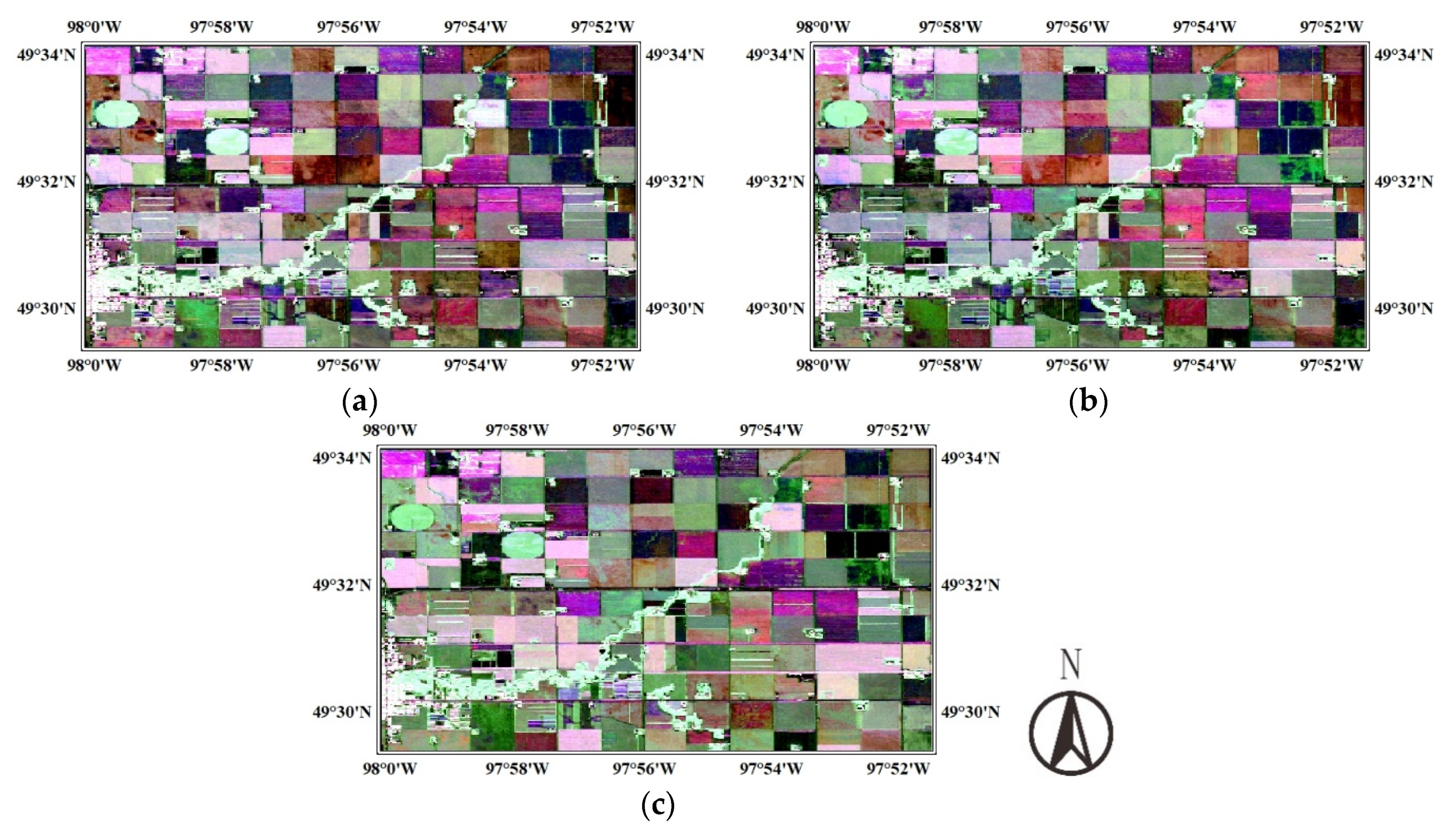
Figure 1. PauliRGB images of multi-temporal UAVSAR dataset. (a) Domain A (2012-07-05); (b) Domain B (2012-07-08); (c) Domain C (2012-07-17).
Remotesensing 12 00658 g001
Figure 2. Ground truth map and classification maps in Winnipeg (SD: A -> TD: B), generated by different methods: (a) Ground truth; (b) DAC; (c) TCA+DAC; (d) SSTCA+DAC; (e) MIDA+DAC; (f) SMIDA+DAC; (g) SMbDA+DAC; (h) WSMbDA+DAC.
Remotesensing 12 00658 g002aRemotesensing 12 00658 g002b
Figure 3. Ground truth map and classification maps in Winnipeg (SD: B -> TD: A), generated by different methods: (a) Ground truth; (b) DAC; (c) TCA+DAC; (d) SSTCA+DAC; (e) MIDA+DAC; (f) SMIDA+DAC; (g) SmbDA+DAC; (h) WSMbDA+DAC.
Remotesensing 12 00658 g003
Figure 4. Ground truth map and classification maps in Winnipeg (SD: A -> TD: C), generated by different methods: (a) Ground truth; (b) DAC; (c) TCA+DAC; (d) SSTCA+DAC; (e) MIDA+DAC; (f) SMIDA+DAC; (g) SMbDA+DAC; (h) WSMbDA+DAC.
Remotesensing 12 00658 g004
Figure 5. Ground truth map and classification maps in Winnipeg (SD: C -> TD: A), generated by different methods: (a) Ground truth; (b) DAC; (c) TCA+DAC; (d) SSTCA+DAC; (e) MIDA+DAC; (f) SMIDA+DAC; (g) SMbDA+DAC; (h) WSMbDA+DAC.
Remotesensing 12 00658 g005
Figure 6. Ground truth map and classification maps in Winnipeg (SD: B -> TD: C), generated by different methods: (a) Ground truth; (b) DAC; (c) TCA+DAC; (d) SSTCA+DAC; (e) MIDA+DAC; (f) SMIDA+DAC; (g) SMbDA+DAC; (h) WSMbDA+DAC.
Remotesensing 12 00658 g006aRemotesensing 12 00658 g006b
Figure 7. Ground truth map and classification maps in Winnipeg (SD: C -> TD: B), generated by different methods: (a) Ground truth; (b) DAC; (c) TCA+DAC; (d) SSTCA+DAC; (e) MIDA+DAC; (f) SMIDA+DAC; (g) SMbDA+DAC; (h) WSMbDA+DAC.
Remotesensing 12 00658 g007aRemotesensing 12 00658 g007b
Figure 8. PauliRGB images of multi-temporal Radarsat-2 dataset and ground truth map in 2012. (a) Domain A (2012-09-01); (b) Domain B (2013-06-16); (c) Domain C (2013-07-10); (d) Domain D (2013-08-03); (e) Ground truth map of Domain A.
Remotesensing 12 00658 g008
Figure 9. Ground truth map and classification maps in Erguna (SD: A -> TD: B), generated by different methods: (a) Ground truth; (b) DAC; (c) TCA+DAC; (d) SSTCA+DAC; (e) MIDA+DAC; (f) SMIDA+DAC; (g) SMbDA+DAC; (h) WSMbDA+DAC.
Remotesensing 12 00658 g009
Figure 10. Ground truth map and classification maps in Erguna (SD: A -> TD: C), generated by different methods: (a) Ground truth; (b) DAC; (c) TCA+DAC; (d) SSTCA+DAC; (e) MIDA+DAC; (f) SMIDA+DAC; (g) SMbDA+DAC; (h) WSMbDA+DAC.
Remotesensing 12 00658 g010
Figure 11. Ground truth map and classification maps in Erguna (SD: A -> TD: D), generated by different methods: (a) Ground truth; (b) DAC; (c) TCA+DAC; (d) SSTCA+DAC; (e) MIDA+DAC; (f) SMIDA+DAC; (g) SMbDA+DAC; (h) WSMbDA+DAC.
Remotesensing 12 00658 g011
Table 1. Precision evaluation results in Winnipeg.
MethodA->B (OA)A->B (Kappa)B->A (OA)B->A (Kappa)A->C (OA)A->C (Kappa)
DAC0.7530.6560.6790.5250.5970.440
TCA0.7990.7230.8290.7610.6450.517
SSTCA0.8090.7370.8390.7740.6670.546
MIDA0.7880.7050.7860.6950.6330.504
SMIDA0.7880.7050.7980.7170.6550.539
SMbDA0.8170.7490.8450.7850.6990.592
WSMbDA0.8700.8210.8960.8540.8430.786
MethodC->A (OA)C->A (Kappa)B->C (OA)B->C (Kappa)C->B (OA)C->B (Kappa)
DAC0.7010.5710.6660.5270.7340.637
TCA0.6800.5650.7370.6400.7350.638
SSTCA0.6840.5700.7730.6860.7350.638
MIDA0.7020.5690.7150.6100.7660.677
SMIDA0.7200.6100.7150.6100.7660.677
SMbDA0.7120.5940.7640.6750.7420.649
WSMbDA0.7580.6660.8570.8040.7650.675
Table 2. Precision evaluation results in Erguna.
MethodA->B (OA)A->B (Kappa)A->C (OA)A->C (Kappa)A->D (OA)A->D (Kappa)
DAC0.117-0.0120.126-0.0090.2040.010
TCA0.4860.3210.5900.4620.7130.608
SSTCA0.4920.3270.6070.4680.7130.608
MIDA0.5080.3480.5670.4320.7760.686
SMIDA0.5080.3480.6000.4770.7760.686
SMbDA0.5290.3690.6360.5240.7580.666
WSMbDA0.6670.5490.8410.7750.8080.733