A Novel ENSO Monitoring Method using Precipitable Water Vapor and Temperature in Southeast China

Abstract

Southeast China, a non-core region influenced by the El Niño–Southern Oscillation (ENSO), has been seldom investigated before. However, the occurrence of ENSO will affect the redistribution of precipitation and the temperature (T) spatial pattern on a global scale. This condition will further lead to flood or drought disasters in Southeast China. Therefore, the method of monitoring the occurrence of ENSO is important and is the focus of this paper. The spatiotemporal characteristics of precipitable water vapor (PWV) and T are first analyzed during ENSO using the empirical orthogonal function (EOF). The results showed that a high correlation spatiotemporal consistency exist between PWV and T. The response thresholds of PWV and T to ENSO are determined by moving the window correlation analysis (MWCA). If the sea surface temperature anomaly (SSTA) at the Niño 3.4 region exceeded the ranges of (−1.17°C, 1.04°C) and (−1.15°C, 1.09°C), it could cause the anomalous change of PWV and T in Southeast China. Multichannel singular spectral analysis (MSSA) is introduced to analyze the multi-type signals (tendency, period, and anomaly) of PWV and T over the period of 1979–2017. The results showed that the annual abnormal signal and envelope line fluctuation of PWV and T agreed well in most cases with the change in SSTA. Therefore, a standard PWV and T index (SPTI) is proposed on the basis of the results to monitor ENSO events. The PWV and T data derived from the grid-based European Center for Medium-Range Weather Forecasting (ECMWF) reanalysis products and GNSS/RS stations in Southeast China were used to validate the performance of the proposed SPTI. Experimental results revealed that the time series of average SPTI calculated in Southeast China corresponded well to that of SSTA with a correlation coefficient of 0.66 over the period of 1979–2017. The PWV values derived from the Global Navigation Satellite System (GNSS) and radiosonde data at two specific stations (WUHN and 45004) were also used to calculate the SPTI. The results showed that the correlation coefficients between SPTI and SSTA were 0.73 and 0.71, respectively. Such results indicate the capacity of the proposed SPTI to monitor the ENSO in Southeast China.

1. Introduction

Water vapor is a major driving force of weather change and atmospheric circulation, and its dynamic trend is an important factor affecting climate and weather prediction [1,2,3]. According to the Clausius–Clapeyron (C-C) equation, a rise of 1 K in atmospheric temperature (T) will result in a 7% increase in water vapor when the relative humidity is regarded as a constant [4]. A total of 7% K^-1 exits deviations in the tropics and mid-latitude, could be canceled in the global mean [5]. An increase of precipitable water vapor (PWV) will cause slight climate change in China, which is the focus area of this paper [6]. Therefore, better knowledge on the accurate distribution and change in atmospheric water vapor is important for climate research and weather prediction.

Techniques, such as radio sounding and water vapor radiometer, have been used to retrieve precipitable water vapor (PWV) for reflecting the variation of atmospheric water vapor. However, these techniques are restricted by their shortcomings. For example, radiosonde (RS) provides water vapor distribution products with limited horizontal and temporal resolution. The general distance between the adjacent sounding stations are nearly 200–300 km, and their sounding balloons are launched 2–4 times a day. Therefore, PWV obtained from RS is used primarily for data calibration [7]. PWV can also be derived from reanalysis products, which use advanced data assimilation technology and provide variables of global atmospheric circulation with high spatial integrity and continuity of data [8,9,10]. However, the accuracy and quality of such PWV need further verification. Since [11] proposed the conception of PWV retrieval using the observations gathered from the Global Navigation Satellite System (GNSS), GNSS meteorology has rapidly developed. Compared with traditional techniques, PWV derived from GNSS observations is characterized by all weather conditions, high precision, high temporal resolution, and low cost [12,13].

The phenomenon of the El Niño–Southern Oscillation (ENSO) is a disturbing normal weather pattern that causes severe drought, floods, tropical cyclones, forest fires, and extreme weather events around the world [14]. [15] reported that the ENSO occurred at a sea surface temperature anomaly (SSTA) value at the Niño 3.4 region, lasting for five months or longer than 0.4 °C, whereas La Niña occurred at the value of a continuous value for five months or more than the time of less than −0.4°C. ENSO has an independent influence on the winter rainfall over Southern China [16,17,18,19]. The anomalous southwesterly winds occur along the southeast coast of China in El Niño years. These anomalous winds substantially enhance the moisture supply to Southern China (SC) and contribute to an increase in January, February, and March (JFM) rainfall in the region [16,19]. Furthermore, [16] found that ENSO has a dominant contribution to temperature anomalies at the upper level, which may enhance convective instability over South China and further contribute to an increase in JFM rainfall over SC. Conversely, Western China and Northern China experienced a high drought risk and a low flood risk in the developing fall of El Niño [20]. Southern China is an important economic zone in China and is densely populated. The abnormal rainfall in winter and spring has a great impact on the economy and human activities. In addition, the East Asian winter monsoon (EAWM) and South China Sea (SCS) sea surface temperature (SST) affects the cold season rainfall in Eastern China [16,17]. EAWM, one of the most influential components of the global climate system, which could induce circulation and further affects the winter season climate in China [17,21]. Among the many affecting parameters of EAWM, the change in tropical SST associated with ENSOs may be a major factor [22]. When the ENSO strengthens, there is a rainfall surplus in Southern and East-Central China and deficits in Northern China [20]. Therefore, ENSO has seriously affected the drought and flood in Eastern and Southern China [22,23,24].

The contribution of ENSO to rainfall and T change has gradually attracted the attention of academic communities [25,26]. Some studies have shown that climate change is correlated with PWV and T [3,4,27]. [28] found that inter-annual variations of tropical water vapor are correlated with T. [3] found that ENSOs significantly affect the change in GNSS-derived PWV and that a 1 K rise in sea surface T will cause an 11% increase in PWV. [29] found PWV data can effectively estimate surface wet and dry changes. These studies have shown that PWV can be used to monitor meteorological drought/flood. Currently, SPI (standard precipitation index), SPEI (standard precipitation evapotranspiration index), and scPDSI (self-calibrating Palmer Drought Severity Index) can generally be used to monitor drought/flood. However, these three indexes have some shortcomings. SPI does not consider the role of T in future drought conditions. The calculation process of SPEI is complex, wherein the key parameter (potential evapotranspiration) is calculated on the basis of the empirical model rather than measured data [30]. ScPDSI is vulnerable to the strong impact of calibration cycles and produces inaccurate estimates at high altitudes and in winter [31,32]. Therefore, it is necessary to develop a new index to monitor drought/flood.

In this study, the spatiotemporal characteristics of PWV and T were first analyzed based on the empirical orthogonal function (EOF) method in Southeast China over the period of 1979–2017, which showed that the time coefficients of PWV and T first mode had a high correlation with SSTA, with values of −0.54 and −0.55, respectively. Then, the response thresholds of anomalous change of PWV and T in Southeast China were determined by moving window correlation analysis (MWCA), and the thresholds were credible based on the experiment data period (1979–2017) and the percentile method. Finally, a novel index, namely, standard PWV and T index (SPTI), is proposed to monitor the effect of ENSO on the anomalous change of PWV and T in Southeast China. The PWV and T are used, and their contributions to SPTI are determined by multichannel singular spectral analysis (MSSA). In addition, the proposed SPTI is validated using ECMWF, GNSS, and RS data over the different period, and the results show a good performance of the proposed index.

2. Materials and Methods

2.1. Materials Description

A total of 5 kinds of data (PWV, T, SST, solar radiation, and SSTA) were used in this study, and the specific spatiotemporal resolutions of these data are summarized in

Table 1. Characteristics of the datasets selected in the experiment.

Data	Spatial and Temporal Resolution		Temporal Coverage/Year	Sources
ECMWF -derived PWV and T	0.5° × 0.5°	monthly	1979–2017	https://www.ecmwf.int/datasets/
SST	2° × 2°	monthly	1979–2017	https://www.esrl.noaa.gov/psd/data/
GNSS-derived PWV	station	hourly	2005–2016	[33]
RS-derived PWV	station	daily	2005–2016	[33]
SSTA	El Niño 3.4	monthly	1979–2017	http://www.cpc.ncep.noaa.gov/
Solar radiation	0.5° × 0.5°	daily	1981–2016	https://rda.ucar.edu/datasets/

. The grid-based PWV and T data in Southeast China were obtained from the fourth-generation reanalysis dataset of the European Center for Medium-Range Weather Forecasting (ECMWF ERA-Interim), and their spatiotemporal resolutions were monthly and 0.5°×0.5°, respectively. ECMWF ERA-Interim covered the corresponding meteorological data from 1979 to 2–3 months before the present. The PWV data at some GNSS and RS stations were also obtained from the Crustal Movement Observation Network of China (CMONOC) and Integrated Global RS Archive Version 2 dataset, respectively [33]. The corresponding geographical distribution of GNSS and RS stations is presented in Figure 1, where the name are WUHN and 45004, respectively. The corresponding sea surface T (SST) data in the ENSO area were derived from the National Oceanic and Atmospheric Administration (NOAA ERSST v3b) [34], and the spatiotemporal resolutions were monthly and 2°×2°, respectively.

According to previous studies [15,35], both SOI and SSTA could represent ENSO events, but based on two different perspectives, SOI is considered from the aspect of atmosphere, while SSTA is considered from the aspect of sea surface temperature. They are different manifestations of the same phenomenon in two media, and they are two sides of the same body. In our study, only SSTA was selected to reflect the ENSO event. The monthly average SSTA in the El Nino 3.4 area (5°N–5°S, 120°W–170°W) were derived from the National Centers for Environmental Prediction (NCEP). The ENSO happened when the SSTA value lasted for 5 months or longer, being larger than 0.4 °C, while the La Niña happened when the SSTA value lasted for 5 months or longer, being less than −0.4 °C [15]. The solar radiation data in Southeast China was also obtained from the university corporation for atmospheric research to analyze the anomalous variation of T during the ENSO period.

2.2. Empirical Orthogonal Function

The empirical orthogonal function (EOF), which is also called principal component analysis, was first proposed by [36]. Since this theory was introduced into atmospheric, oceanic, and climatic studies by [37], it has been widely used as a convenient and effective theory [38,39]. EOF can decompose the meteorological dataset of spatiotemporal distribution into a pattern sorted by its time variance [40], that is, the original correlated variable field is decomposed into several irrelevant spatial functions and time coefficients [38] without losing the original data information [41], to analyze the spatial structure of the actual field. EOF can also represent the change pattern of a single variable (EOF pattern) and explain the proportion of the total variance of all variables in the dataset [42].

The two main steps of conducting EOF decomposition are to first flatten the original data and then construct the covariance matrix [43]. The matrix form of the spatiotemporal grid data is:

$$X=\left[\begin{array}{cccc}{x}_{11}& x_{12}& \cdots & x_{1n}\\ x_{21}& x_{22}& \cdots & x_{2n}\\ ⋮& ⋮& \ddots & ⋮\\ x_{m1}& x_{m2}& \cdots & x_{mn}\end{array}\right]$$

(1)

where $X(i,j)$ is the observed value corresponding to the position $i$($i\in (1,m)$) and the time $j(j\in (1,n))$. The anomaly field $X_A$ is as follows:

$$X_A=X-{(S^T(\frac{1}{n}S{X}^T))}^T$$

(2)

where $S=(1,\cdots ,1)$ is composed by n numbers of 1. 2): The structure of the covariance matrix $C$ is:

$$C=X_A\cdot X_A{}^T.$$

(3)

2.3. MWCA

MWCA is used to investigate the correlation and non-stationarity relationship among parameters. The value of the moving window is first determined before using MWCA. By moving the selected windows in the dataset analysis, the independent local correlation coefficient for each window can be calculated. Therefore, a smooth time series can be generated and the continuity of each time process can be analyzed [44,45]. In this study, MWCA is introduced to investigate the relationship between monthly PWV/ T and ENSO. The local correlation coefficient is calculated using the following formula:

$$R_{jL}=\frac{\frac{1}{L}{\displaystyle \sum _{j=1}^L(a_j-\overline{a_{jL}})(b_j-\overline{b_{jL}})}}{{\sigma }_{aL}{\sigma }_{bL}}$$

(4)

where $R_{jL}$ is the correlation coefficient of month $j$. $L$ is the selected moving window. $a_j$ and $b_j$ are the independent variables of the $a$ and $b$ of month $j$, respectively. $\overline{a_{jL}}$ and $\overline{b_{jL}}$ are the mean values of $a$ and $b$ in the window $L$, respectively. ${\sigma }_{aL}$ and ${\sigma }_{bL}$ are the standard errors of $a$ and $b$ in the window $L$, respectively.

2.4. MSSA

The singular spectral analysis (SSA) method is an adaptive data filter that eliminates background noise and retains leading statistical significances, such as trends, fluctuations, and noise components [46,47,48]. This method can effectively display the amplitude and offset of the nonlinear trend and periodic term over time in the data time series [3], and was extended to MSSA by [49]. MSSA is an advanced adaptive data method for extracting the trend characteristics of a space and time series and the nonlinear oscillation embedded in the climate time series without prior information about functions or stochastic models. Therefore, it can be flexibly applied to various data and has widely been used in oceanography, meteorology, and climate research [10,50,51]. In this study, the MSSA is used to analyze the PWV and T time series and obtain their periodic signals and anomalous change trend.

The MSSA algorithm is composed of three main steps. Firstly, a grand covariance matrix is calculated. The dataset $N_a(f)(a=1,\cdots ,$$A;f=1,\cdots ,F)$, $A$ is the time series or channels, and $F$ is the size of every time series or channel. A data trajectory matrix is composed by selecting a lag-window $M$.

$$D_a=\left[\begin{array}{cccc}{N}_a(1)& N_a(2)& \cdots & N_a(M)\\ N_a(2)& N_a(3)& \cdots & N_a(M+1)\\ ⋮& ⋮& \ddots & ⋮\\ N_a(F\prime )& N_a(F\prime +1)& \cdots & N_a(F)\end{array}\right]$$

(5)

where $F\prime =F-M+1$ is the size of the overlapping views of the every time series or channel. The covariance matrix $K_{a,a\prime }$ between channels $N_a(f)$ and $N_{a\prime }(f)$ is $K_{a,a\prime }=\frac{1}{F\prime }{D}_a{}^T{D}_{a\prime }$. These matrices are the blocks of the grand matrix $\tilde{D}$ (size:$A\times M,A\times M$):

$$\tilde{D}=\left[\begin{array}{cccc}{K}_{1,1}& K_{1,2}& \cdots & K_{1,A}\\ K_{2,1}& K_{2,2}& \cdots & K_{2,A}\\ ⋮& ⋮& \ddots & ⋮\\ K_{A,1}& K_{A,2}& \cdots & K_{A,A}\end{array}\right]$$

(6)

The second and third steps are to calculate the spatiotemporal principal components (ST-PCs) and the reconstructed time series, respectively. The eigenvalues ${\lambda }^L$ and eigenvectors $E^L$ are obtained according to $\tilde{D}{E}^L={\lambda }^L{E}^L$($L=1,2,\cdots ,A\times M$). $E^L$ are also called the spatiotemporal empirical orthogonal functions (ST-EOFs). Then the time series is projected onto the ST-EOFs to get the ST-PCs:

$$A^L(f)={\displaystyle \sum _{i=1}^M{\displaystyle \sum _{a=1}^A{N}_a}}(f+i-1)E_a^L(i),1\le f\le F\prime$$

(7)

where $L$ and $a$ is $L\mathrm{th}$ eigenvector and $a\mathrm{th}$ channel, respectively. Finally to partly reconstruct the time series $N_a(f)$ [46] based on the ST-PCs ($A^L$) and ST-EOFs ($E_a^L$):

$$R_a^L(f)=\{\begin{array}{cc}\frac{1}{f}{\displaystyle \sum _{i=1}^f{A}^L}(f-i+1)E_a^L(i)& 1\le f\le M-1\\ \frac{1}{M}{\displaystyle \sum _{i=1}^M{A}^L}(f-i+1)E_a^L(i)& M\le f\le F\prime \\ \frac{1}{F-f+1}{\displaystyle \sum _{i=f-F+M}^M{A}^L}(f-i+1)E_a^L(i)& F\prime +1\le f\le F\end{array}.$$

(8)

The partial signal could be reconstructed from Equation (7). More details of the MSSA can be found in [10].

2.5. Retrieval of PWV Based on the GNSS Observation

The original GNSS observations from the CMONOC were processed using the GAMIT/GLOBK (Ver. 10.4), and the double differences in phase observations were applied [52]. Therefore, the key troposphere parameter, zenith tropospheric delay (ZTD), which consists of zenith hydrostatic delay (ZHD) and zenith wet delay (ZWD), could be estimated. ZHD, which accounts for approximately 90% of ZTD, can be precisely calculated using the surface pressure with the empirical Saastamonien model [53]:

$$Z_{hd}=\frac{0.0022768P_s}{1-0.00266\cos (2\phi )-0.00028H}$$

(9)

where $P_s$ and $\phi$ refer to the surface pressure in hPa and latitude of the GNSS station in radian, respectively. $H$ is the geoid height of the GNSS station in km. A rise in $P_s$ of 1 hPa will only lead to a ZHD error of 0.2 mm [54].

ZWD can thus be obtained by extracting ZHD from ZTD, and the final PWV is calculated by the following formula [55,56]:

$$P_{wv}=\frac{{10}^6\cdot Z_{wd}}{R_g(k_3/T_m+k_2^{\prime }){\rho }_w}$$

(10)

where ${\rho }_w$ is the liquid water density constant with a value of 103 $kg/m^3$, $R_g$, $k_2^{\prime }$, and $k_3$ are constants with values of 461$J\cdot k{g}^{-1}\cdot K^{-1}$, $16.48K/hP{a}^{-1}$, and $(3.776\pm 0.014)\times {10}^5{K}^2/hPa$, respectively. $T_m$ is the weighted average T of atmospheric water vapor in K, and the accurate value can be calculated as:

$$T_m=\frac{{\displaystyle \int (e/T)dz}}{{\displaystyle \int (e/T^2)dz}}$$

(11)

where $e$ is the layered water vapor pressure, $T$ is the layered absolute temperature, and $dz$ is the integral path. Due to the layered meteorological parameters being generally unavailable, an empirical formula proposed by [57] using the surface T was used in this paper:

$$T_m=44.05+0.81T$$

(12)

3. Analysis of Anomalous Variations of PWV and T During ENSO

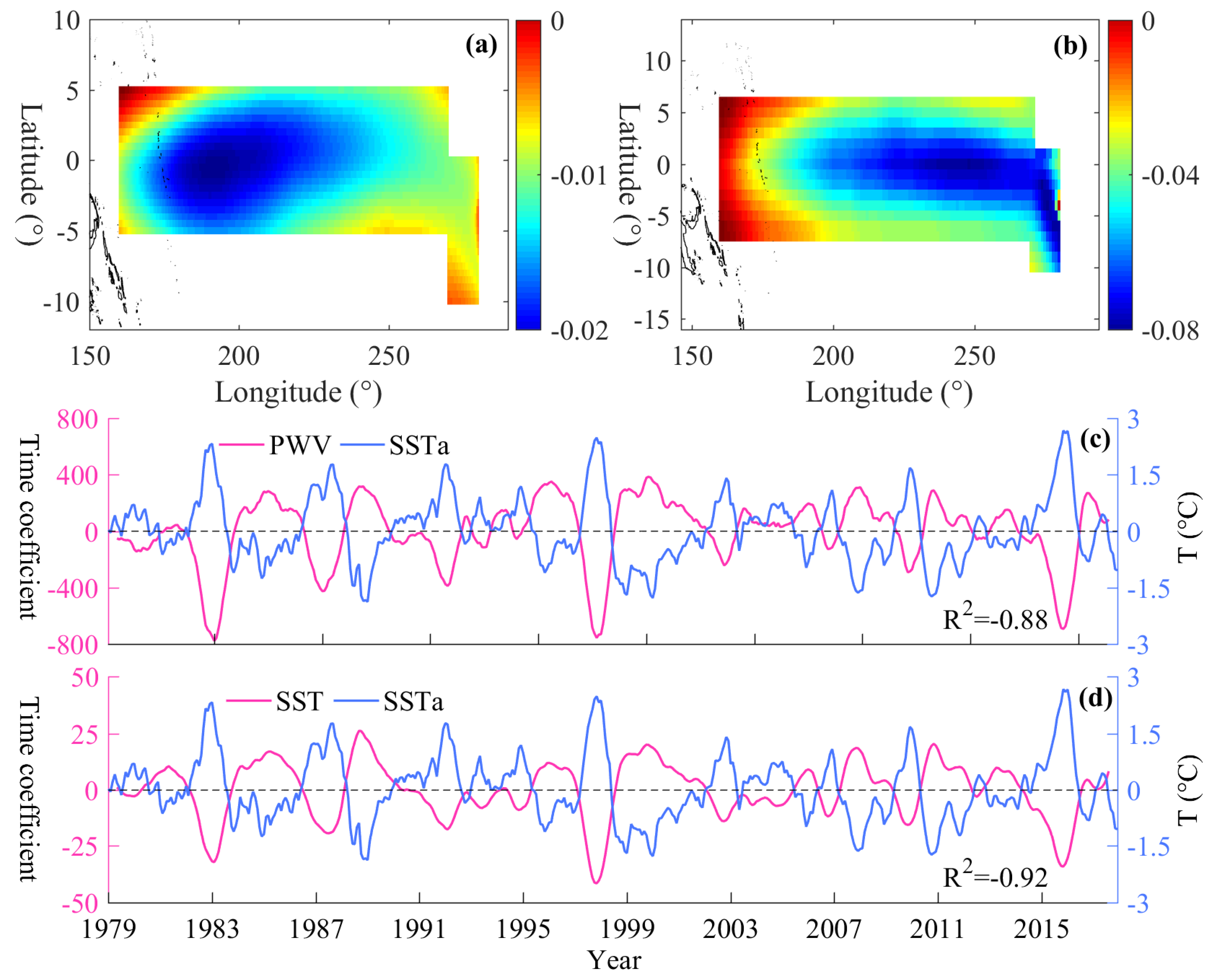
3.1. Spatiotemporal Characteristic Analysis of PWV and SST/T

The anomalous variation of PWV and SST in the El Niño area over the period of 1979–2017 is analyzed initially using EOF to assess the correlation between ENSO and PWV/ T. Figure 2 presents the spatiotemporal pattern of PWV and SST first mode, compared with the time series of SSTA in the El Niño area over the period of 1979–2017. As shown in Figure 2a,b, the spatial distributions of PWV and SST first mode were negative in the El Niño area but with different values. The extreme values of PWV and SST first mode appeared in the Central and Western equatorial Pacific Ocean (150°W–170°E, 4°S–4°N), in the Eastern Equatorial Pacific (95°E–135°W, 2°S–2°N), and Nino 2 area (80°E–87°W, 1°N–5°S), respectively. Numerical results revealed that the variance contribution rates of PWV and SST first mode were 67% and 76%, respectively. Therefore, 67% and 76% of anomalous variations of PWV and SST were affected by the weather system of the same scale, and the variation trend was consistent. Figure 2c and d present the time series of time coefficient of PWV and SST first mode, where the moving average method was used to smooth the time coefficient with a moving window of 9 months. When the time coefficient of PWV and SST first mode was a negative (positive) extreme outlier, the SSTA corresponded to a positive (negative) extreme outlier. The correlation coefficients between the time coefficient of PWV and SST first mode and SSTA were 0.88 and 0.92, respectively. Therefore, the PWV and the SST were affected by ENSO in the El Niño area.

To further analyze whether the anomalous changes of PWV/T were affected by ENSO event in Southeast China, Figure 3 shows the spatiotemporal pattern of PWV and T first mode compared with that of SSTA in Southeast China over the period of 1979–2017. As shown in Figure 3a,b, the spatial distributions of PWV and T first mode were similar in Southeast China but with opposite values. The covariance contribution rates of PWV and T first mode were 70% and 75%, respectively, and both cases passed the North test. Therefore, the spatial pattern of PWV and T in Southeast China had a significant physical significance. The temporal patterns of PWV and T first mode are also presented in Figure 3c,d. The time coefficients of PWV and T first mode had a good consistency with the time series of SSTA. The corresponding coefficients between the time coefficients of PWV and T first mode and SSTA were −0.54 and −0.55, respectively. Such results reveal that the ENSO also had a moderate negative impact on the anomalous variation of PWV and T in Southeast China [58], which means that the increasing of temperature of SST could cause a decrease of PWV and T in Southeast China.

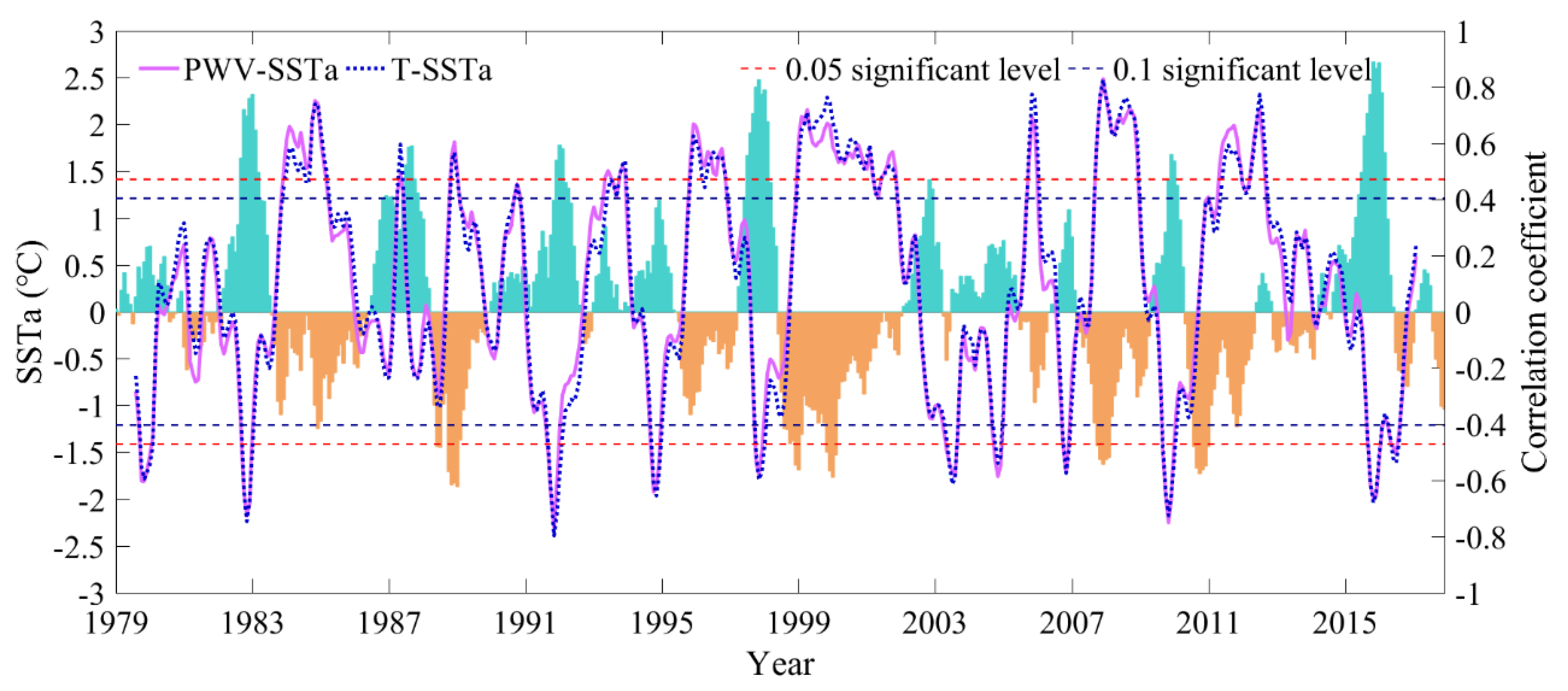
3.2. Determination of Response Thresholds of PWV and T to ENSO in Southeast China

Although China is not the core area affected by ENSO, PWV and T are affected by such an event to a large extent, as discussed in Section 3.1. Therefore, the condition under which ENSO will cause the anomalous variation of PWV and T becomes the focus of this section. The monthly PWV and T were averaged in Southeast China, and MWCA was conducted to explore the relationship between ENSO and PWV/T in Southeast China. A moving window of 18 months was selected following [44]. Therefore, the correlation coefficients between PWV/T and SSTA could be obtained (Figure 4). It can be observed from Figure 4 that the correlation coefficients between PWV-SSTA and T-SSTA were consistent over the period of 1979–2017. In addition, the time series of PWV-SSTA/T-SSTA coefficients and ENSO showed an evident negative correlation. Thus, PWV and T were negatively correlated with a strong El Niño and positively correlated with a strong La Niña (P < 0.05). The maximum values of the correlation coefficients between PWV/T and strong El Nino were larger than −0.55. Therefore, a medium remote correlation existed between ENSO and PWV and T in Southeast China.

A linear fitting was used between SSTA and PWV/T to quantify the impact of ENSO on PWV/T in Southeast China (pink line). For quantitative purposes, the correlation coefficients between the PWV-SSTA/T-SSTA were divided into three parts based on the percentile method. The upper percentile and lower percentile were 75% (upper dotted line) and 25% (lower dotted line), respectively. Figure 5 presents the scatter plots of the correlations of PWV-SSTA/T-SSTA and SSTA. The results show that the response thresholds of PWV to El Niño and La Niña were −1.17°C and 1.04°C, respectively. Therefore, when the SSTA value exceeded −1.17°C or 1.04°C, the anomalous change in PWV in Southeast China was evidently affected by El Niño and La Niña. Figure 5b reveals that the response thresholds of T to El Niño and La Niña were −1.15°C and 1.09°C, respectively. Thus, when the SSTA value exceeded −1.15°C or 1.09°C, the anomalous change in T in Southeast China was evidently affected by El Niño and La Niña.

3.3. Anomalous Analysis of PWV and T during ENSO Period using MSSA

MSSA is used with the experimental windows of 35 [59] to analyze the long-term series PWV and T in Southeast China for obtaining the nonlinear anomalous trend included in PWV and T. Figure 6 presents the first seven components of PWV and T in Southeast China from 1979 to 2017 using MSSA. The PWV and T included the inter-annual trend (RC1), annual (RC2–3), semi-annual (RC4-5), and anomalous (RC6) periods. RC7 may be the noise or unknown signal information.

Table 2. Contribution rates corresponding to the first seven eigenvalues in Southeastern China from 1979 to 2017.

Contribution Rate	Principal Components
	1	2	3	4	5	6	7
Variance Contribution Rate	85.71	7.05	6.68	0.1	0.1	0.01	0.01
Accumulated Variance Contribution Rate	85.71	92.76	99.44	99.54	99.64	99.65	99.67

also gives the variance contribution rates of the first six components. The cumulative variance contribution rate of RC1–3 was 99.44%. Therefore, the changes of PWV and T in Southeast China were primarily driven by trend and annual signals.

Apart from the influence of the trend, annual and semi-annual periods, PWV and T had an evident anomalous variation (RC6) over the period of 1979–2017, as shown in Figure 6. Therefore, Figure 7 presents the time series of anomalous variations of PWV and T derived from RC6 in Figure 6a and b with SSTA in the period 1979–2017 in Southeast China. The anomalous variations of PWV and T showed an upward trend when medium or strong ENSO occurred. Compared with the anomalous variation of T, PWV had a more evident response characteristic to ENSO. Envelope lines of PWV and T were also obtained in Southeast China. The change trend in Southeast China was primarily affected by trend and periodic signals. Therefore, the abnormal time series of PWV and T were obtained by removing the trend and periodic signals. The maximum abnormal value of each year could be determined, and the envelope lines of PWV and T could be obtained by the cubic spline interpolation at other months. Figure 8 presents the envelope lines of PWV and T with SSTA over the period of 1979–2017 in Southeast China. The envelop line of PWV had a good relationship with ENSO. However, the relationship between the envelop line of T and SSTA was slightly poor. This result was acceptable because solar radiation was also an important influencing factor of the T change in Southeast China. For example, the envelop line of T over the period of 2015–2017 showed an evident decreasing trend because the solar radiation in Southeast China in these years decreased by 32% compared with the same data in the previous years.

3.4. Standard PWV and Temperature Index (SPTI)

The above-mentioned analysis of the anomalous variations of PWV and T proved that these variations were related to the ENSO occurring over the period of 1979–2017 in Southeast China. Therefore, the SPTI, which is an index for monitoring ENSO using the anomalous change in PWV and T, is proposed in this section. The specific steps of determining this index are listed as follows:

(1)

The time series of PWV and T is reprocessed by removing the trend and periodic terms using the MSSA;

(2)

The reprocessed PWV and T time series are normalized due to their different magnitudes using the following formula [60]:

$${\tilde{N}}_i=\frac{y_{max}-y_{min}}{N_{max}-N_{\min }}\cdot (N_i-N_{\min })+y_{min}$$

(13)

where $y_{max}$ and $y_{min}$ are the maximum and minimum values of the mapping range, which usually are 1 and −1, respectively. $N_{max}$ and $N_{\min }$ are the maximum and minimum values of the N vector, respectively. $N_i$ and ${\tilde{N}}_i$ are the $i\mathrm{th}$ value in the N vector and the normalized value corresponding to the $i\mathrm{th}$ value in the N vector, respectively;

(3)

The optimal weightings of the normalized PWV and T time series are determined using the MSSA method. The anomalous variations (RC6 in Figure 6) of PWV and T obtained using the MSSA are correlated with ENSO. Therefore, the reprocessed PWV and T time series are used to obtain the variance contribution rates of abnormal signals. Then, these rates are used to determine the optimal weightings between PWV and T. The weighted normalized value for calculating the SPTI can be obtained and expressed as:

$$NPT=({\tilde{N}}_{PWV}\times P_{PWV}+{\tilde{N}}_T\times P_T)/(P_{PWV}+P_T)$$

(14)

where ${\tilde{N}}_{PWV}$ and ${\tilde{N}}_T$ are the normalized PWV and T values, respectively. $P_{PWV}$ and $P_T$ are the weightings of PWV and T, respectively. $NPT$ is the normalized PWV and T value, which is used to calculate the SPTI based on the Z score method [61]. The Z score is the deviation from the mean in units of the standard deviation. The SPTI time series is calculated using the monthly $N_{PT}$ value over the period of 1979–2017 as follows:

$$SPT{I}_{mn}=\frac{NP{T}_{mn}-\overline{NP{T}_m}}{{\sigma }_m}$$

(15)

where $SPT{I}_{mn}$ refers to the monthly SPTI value during month $m$ for year $n$. $\overline{NP{T}_m}$ is the mean NPT during month $m$ over $n$ years. ${\sigma }_m$ is the standard deviation of NPT during month $m$ over $n$ years, which is used to reflect the degree of deviation of PWV and T from normal value.

4. Validation of the SPTI for Monitoring ENSO

4.1. Validation of the SPTI using the ECMWF Data

The monthly PWV and T in Southeast China were derived from grid-based ECMWF ERA-Interim products. The mean PWV and T in Southeast China were obtained and used to calculate the month SPTI following the steps in Section 3.4. Figure 9 gives the time series of monthly SPTI in Southeast China with SSTA over the period of 1979–2017. It can be observed from Figure 9 that the SPTI had a good response to the occurrence of ENSO. The proposed SPTI showed an evident upward trend when strong El Niño occurred in 1983, 1987, 1998, 2009, and 2016. A similar downward trend is presented when the strong La Niña happened in 1989, 1996, 2008, and 2011. In addition, the proposed SPTI showed a strong correlation with SSTA, in which the correlation coefficient was 0.66. Such results verify the potential capacity of the proposed SPTI for monitoring ENSO on the basis of the anomalous variations of PWV and T data.

4.2. Validation of SPTI At GNSS/RS Stations

High-precision PWV data can also be obtained using GNSS or radio sounding techniques at specific stations. In consideration of this fact, SPTI calculated using GNSS-/RS-derived PWV with SSTA is compared. One GNSS station (WUHN) and a RS station (45004) were selected in Southeast China. The specific geographic locations of selected stations are shown in Figure 1. The T and PWV data at specific GNSS/RS stations were also interpolated using the grid-based ERA-Interim product. Figure 10 presents the time series of monthly SPTI calculated using ERA-Interim/GNSS/RS data with SSTA at GNSS and RS stations (WUHN and 45004, respectively) over the period of 2005–2016. This period is selected because only the GNSS- and RS-derived PWV could be obtained in this period.

As shown in Figure 10a, the time series of GNSS-/ERA-Interim-derived SPTI at WUHN station were similar, and both time series had a good consistency with those of SSTA. The correlation coefficient between GNSS-derived SPTI and SSTA was 0.73, while that between ERA-Interim-derived SPTI and SSTA was 0.59. Similar results could also be observed from Figure 10b, that is, the RS-derived SPTI at 45004 station agreed well with that from ERA-Interim, and the coefficients between RS-/ERA-Interim-derived SPTI and SSTA were both 0.71. In addition, the change trend of ENSO could be reflected by SPTIs derived from GNSS and RS stations. This condition further verifies the good performance of the proposed SPTI. Such results obtained above also show that the tele-correlation effect of ENSOs on PWV and T anomalies in Southeast China can be monitored.

5. Conclusions

In this paper, we firstly proposed a novel index SPTI for monitoring the impact of ENSO over Southeast China, and its performance was then validated in the entire area of Southeast China and at GNSS and RS stations, respectively. The EOF method was first introduced to analyze the correlation between SSTA and PWV/T. The results indicated that the time coefficients of PWV and T first mode showed a high correlation with SSTA with coefficients of −0.54 and −0.55, respectively. MWCA was then applied to quantify the extent to which ENSO affected PWV/T in Southeast China. The response thresholds of PWV to El Niño /La Niña were −1.17 °C and 1.04 °C, respectively. Meanwhile, those of T to El Niño /La Niña were −1.15 °C and 1.09 °C, respectively. In addition, MSSA was used to extract the anomalous signal in PWV and T. The results showed that this signal had a high correlation with SSTA. Therefore, SPTI was proposed using the anomalous change in PWV and T to monitor the ENSO.

The performance of SPTI was validated using the ECMWF ERA-Interim data in the whole of Southeast China over the period of 1979–2017. A comparison showed that SPTI had a good consistency with SSTA and that the coefficient was 0.66. The GNSS- and RS-derived SPTIs at WUHN and 45004 stations were also calculated in 2005–2016 compared with the corresponding SSTA. A similar result was obtained, that is, a good correlation existed between GNSS-/RS-derived SPTIs and SSTA with correlation coefficients of 0.73 and 0.71, respectively. Such comparisons in the whole of Southeast China and specific stations verify the capacity of the proposed SPTI in monitoring ENSO.

References

1. Chung, E.-S.; Soden, B.; Sohn, B.J.; Shi, L. Upper-tropospheric moistening in response to anthropogenic warming. Proc. Natl. Acad. Sci. USA 2014, 111, 11636–11641. [Google Scholar] [CrossRef] [Green Version]
2. Guerova, G.; Jones, J.; Douša, J.; Dick, G.; De Haan, S.; Pottiaux, E.; Bock, O.; Pacione, R.; Elgered, G.; Vedel, H.; et al. Review of the state of the art and future prospects of the ground-based GNSS meteorology in Europe. Atmospheric Meas. Tech. 2016, 9, 5385–5406. [Google Scholar] [CrossRef] [Green Version]
3. Wang, X.; Zhang, K.; Wu, S.; Li, Z.; Cheng, Y.; Li, L.; Yuan, H. The correlation between GNSS-derived precipitable water vapor and sea surface temperature and its responses to El Niño–Southern Oscillation. Remote. Sens. Environ. 2018, 216, 1–12. [Google Scholar] [CrossRef]
4. Trenberth, K.E.; Dai, A.; Rasmussen, R.M.; Parsons, D.B. The Changing Character of Precipitation. Bull. Am. Meteorol. Soc. 2003, 84, 1205–1218. [Google Scholar] [CrossRef]
5. O’Gorman, P.A.; Muller, C.J. How closely do changes in surface and column water vapor follow Clausius–Clapeyron scaling in climate change simulations? Environ. Res. Lett. 2010, 5, 025207. [Google Scholar] [CrossRef]
6. Xie, B.; Zhang, Q.; Ying, Y. Trends in Precipitable Water and Relative Humidity in China: 1979–2005. J. Appl. Meteorol. Clim. 2011, 50, 1985–1994. [Google Scholar] [CrossRef]
7. Guerova, G. Derivation of Integrated Water Vapor (IWV) from the ground-based GPS estimates of Zenith Total Delay (ZTD); Department of Microwave Physics, Institute of Applied Physics, University of Bern: Bern, Switzerland, 2003. [Google Scholar]
8. Bengtsson, L.; Hagemann, S.; Hodges, K.I. Can climate trends be calculated from reanalysis data? J. Geophys. Res. 2004, 109, D11111. [Google Scholar] [CrossRef] [Green Version]
9. Dessler, A.E.; Davis, S.M. Trends in tropospheric humidity from reanalysis systems. J. Geophys. Res. 2010, 115, D19127. [Google Scholar] [CrossRef]
10. Zhang, B.; Liu, L.; Khan, S.A.; Van Dam, T.; Zhang, E.; Yao, Y. Transient Variations in Glacial Mass Near Upernavik Isstrøm (West Greenland) Detected by the Combined Use of GPS and GRACE Data. J. Geophys. Res. Solid Earth 2017, 122, 10–626. [Google Scholar] [CrossRef] [Green Version]
11. Bevis, M.; Businger, S.; Herring, T.A.; Rocken, C.; Anthes, R.A.; Ware, R.H. GPS meteorology: Remote sensing of atmospheric water vapor using the global positioning system. J. Geophys. Res. Atmos. 1992, 97, 15787. [Google Scholar] [CrossRef]
12. Nilsson, T.; Gradinarsky, L. Water vapor tomography using GPS phase observations: Simulation results. IEEE Trans. Geosci. Remote. Sens. 2006, 44, 2927–2941. [Google Scholar] [CrossRef]
13. Jin, S.; Park, J.-U.; Cho, J.-H.; Park, P.-H. Seasonal variability of GPS-derived zenith tropospheric delay (1994–2006) and climate implications. J. Geophys. Res. 2007, 112, D09110. [Google Scholar] [CrossRef]
14. McPhaden, M.J. El Nino and La Nina: Causes and global consequences. Encycl. Glob. Environ. Chang. 2002, 1, 1–17. [Google Scholar]
15. Trenberth, K.E.; Hoar, T.J. El Niño and climate change. Geophys. Res. Lett. 1997, 24, 3057–3060. [Google Scholar] [CrossRef]
16. Zhou, L.-T.; Tam, C.-Y.; Zhou, W.; Chan, J.C.L. Influence of South China Sea SST and the ENSO on winter rainfall over South China. Adv. Atmos. Sci. 2010, 27, 832–844. [Google Scholar] [CrossRef]
17. Zhou, L.-T.; Wu, R. Respective impacts of the East Asian winter monsoon and ENSO on winter rainfall in China. J. Geophys. Res. 2010, 115, D02107. [Google Scholar] [CrossRef]
18. Karori, M.A.; Li, J.; Jin, F.-F. The Asymmetric Influence of the Two Types of El Niño and La Niña on Summer Rainfall over Southeast China. J. Clim. 2013, 26, 4567–4582. [Google Scholar] [CrossRef]
19. Zhang, L.; Fraedrich, K.; Zhu, X.; Frank, S.; Zhi, X. Interannual variability of winter precipitation in Southeast China. Theor. Appl. Climatol. 2015, 119, 229–238. [Google Scholar] [CrossRef]
20. Li, X.; Zhou, W.; Chen, Y.D. Assessment of Regional Drought Trend and Risk over China: A Drought Climate Division Perspective. J. Clim. 2015, 28, 7025–7037. [Google Scholar] [CrossRef]
21. Huang, R.; Chen, J.; Huang, G. Characteristics and variations of the East Asian monsoon system and its impacts on climate disasters in China. Adv. Atmospheric Sci. 2007, 24, 993–1023. [Google Scholar] [CrossRef]
22. Sun, C.; Yang, S. Persistent severe drought in southern China during winter-spring 2011: Large-scale circulation patterns and possible impacting factors. J. Geophys. Res. 2012, 117, D10112. [Google Scholar] [CrossRef]
23. Huang, R.; Wu, Y. The influence of ENSO on the summer climate change in China and its mechanism. Adv. Atmos. Sci. 1989, 6, 21–32. [Google Scholar]
24. Zhang, R.; Sumi, A. Moisture circulation over East Asia during the El Niño episode in northern winter, spring, and autumn. J. Meteorol. Soc. Jpn. 2002, 80, 213–227. [Google Scholar] [CrossRef] [Green Version]
25. Chowdhury, M.R. The El Niño-Southern Oscillation (ENSO) and seasonal flooding-Bangladesh. Theor. Appl. Climatol. 2003, 76, 105–124. [Google Scholar] [CrossRef]
26. Tong, J.; Zhang, Q.; Zhu, D.M.; Wu, Y.J. Yangtze floods and droughts (China) and teleconnections with ENSO activities (1470–2003). Quat. Int. 2006, 144, 29–37. [Google Scholar] [CrossRef]
27. AlShawaf, F.; Balidakis, K.; Dick, G.; Heise, S.; Wickert, J. Estimating trends in atmospheric water vapor and temperature time series over Germany. Atmos. Meas. Tech. 2017, 10, 3117–3132. [Google Scholar] [CrossRef] [Green Version]
28. Sun, D.Z.; Held, I.M. A comparison of modeled and observed relationships between interannual variations of water vapor and temperature. J. Clim. 1995, 9, 665–675. [Google Scholar] [CrossRef] [Green Version]
29. Bordi, I.; Zhu, X.; Fraedrich, K. Precipitable water vapor and its relationship with the Standardized Precipitation Index: Ground-based GPS measurements and reanalysis data. Theor. Appl. Climatol. 2016, 123, 263–275. [Google Scholar] [CrossRef]
30. Vicente-Serrano, S.M.; Beguería, S.; López-Moreno, J.I. A Multiscalar Drought Index Sensitive to Global Warming: The Standardized Precipitation Evapotranspiration Index. J. Clim. 2010, 23, 1696–1718. [Google Scholar] [CrossRef] [Green Version]
31. Akinremi, O.O.; McGinn, S.M.; Barr, A.G. Evaluation of the Palmer Drought Index on the Canadian Prairies. J. Clim. 1996, 9, 897–905. [Google Scholar] [CrossRef] [Green Version]
32. Weber, L.; Nkemdirim, L.C. The Palmer drought severity index revisited. Geogr. Ann. 1998, 80, 153–172. [Google Scholar] [CrossRef]
33. Zhao, Q.; Yao, Y.; Yao, W.; Zhang, S. GNSS-derived PWV and comparison with radiosonde and ECMWF ERA-Interim data over mainland China. J. Atmos. Sol. Terr. Phys. 2019, 182, 85–92. [Google Scholar] [CrossRef]
34. Smith, T.M.; Reynolds, R.W.; Peterson, T.C.; Lawrimore, J. Improvements to NOAA’s Historical Merged Land–Ocean Surface Temperature Analysis (1880–2006). J. Clim. 2008, 21, 2283–2296. [Google Scholar] [CrossRef]
35. Camp, C.D.; Tung, K.-K. Stratospheric polar warming by ENSO in winter: A statistical study. Geophys. Res. Lett. 2007, 34, L04809. [Google Scholar] [CrossRef] [Green Version]
36. Pearson, K. LIII. On lines and planes of closest fit to systems of points in space. Lond. Edinb. Dublin Philos. Mag. J. Sci. 1902, 2, 559–572. [Google Scholar] [CrossRef] [Green Version]
37. Lorenz, E.N. Empirical Orthogonal Functions and Statistical Weather Prediction; Massachusetts Institute of Technology, Department of Meteorology: Cambridge, MA, USA, 1956. [Google Scholar]
38. Weare, B.C.; Navato, A.R.; Newell, R.E. Empirical Orthogonal Analysis of Pacific Sea Surface Temperatures. J. Phys. Oceanogr. 1976, 6, 671–678. [Google Scholar] [CrossRef] [Green Version]
39. Kidson, J.W. Eigenvector Analysis of Monthly Mean Surface Data. Mon. Weather. Rev. 1975, 103, 177–186. [Google Scholar] [CrossRef] [Green Version]
40. Lagerloef, G.S.E.; Bernstein, R.L. Empirical orthogonal function analysis of advanced very high resolution radiometer surface temperature patterns in Santa Barbara Channel. J. Geophys. Res. Oceans 1988, 93, 6863. [Google Scholar] [CrossRef]
41. Hannachi, A.; O’Neill, A. Atmospheric multiple equilibria and non-Gaussian behaviour in model simulations. Q. J. R. Meteorol. Soc. 2001, 127, 939–958. [Google Scholar] [CrossRef]
42. Kim, S.E.; Seo, I.W.; Choi, S.Y. Assessment of water quality variation of a monitoring network using exploratory factor analysis and empirical orthogonal function. Environ. Model. Softw. 2017, 94, 21–35. [Google Scholar] [CrossRef]
43. Hannachi, A.; Jolliffe, I.T.; Stephenson, D.B. Empirical orthogonal functions and related techniques in atmospheric science: A review. Int. J. Clim. 2007, 27, 1119–1152. [Google Scholar] [CrossRef]
44. Propastin, P. Monitoring System for Assessment of Vegetation Sensitivity to El-Niño over Africa; Springer Science and Business Media LLC: Berlin, German, 2009; pp. 329–344. [Google Scholar]
45. Zhao, Q.; Ma, X.; Yao, W.; Liu, Y.; Yao, Y. Anomaly variation of vegetation and its influencing factors in Mainland China during ENSO period. IEEE Access 2019, 8, 721–734. [Google Scholar] [CrossRef]
46. Ghil, M.; Vautard, R. Interdecadal oscillations and the warming trend in global temperature time series. Nature 1991, 350, 324–327. [Google Scholar] [CrossRef]
47. Vautard, R.; Yiou, P.; Ghil, M. Singular-spectrum analysis: A toolkit for short, noisy chaotic signals. Phys. D Nonlinear Phenom. 1992, 58, 95–126. [Google Scholar] [CrossRef]
48. Semiromi, M.T.; Ghasemian, D. Reconstruction of Water Infiltration Rate Reducibility in Response to Suspended Solid Characteristics Using Singular Spectrum Analysis: An Application to the Caspian Sea Coast of Nur, Iran. Hydrology 2018, 5, 59. [Google Scholar] [CrossRef] [Green Version]
49. Plaut, G.; Vautard, R. Spells of Low-Frequency Oscillations and Weather Regimes in the Northern Hemisphere. J. Atmos. Sci. 1994, 51, 210–236. [Google Scholar] [CrossRef] [Green Version]
50. Huang, W.; Wang, R.; Yuan, Y.; Gan, S.; Chen, Y. Signal extraction using randomized-order multichannel singular spectrum analysis. Geophysics 2016, 82, V69–V84. [Google Scholar] [CrossRef]
51. Ghil, M.; Allen, M.R.; Dettinger, M.D.; Ide, K.; Kondrashov, D.; Mann, M.E.; Robertson, A.W.; Saunders, A.; Tian, Y.; Varadi, F.; et al. Advanced spectral methods for climatic time series. Rev. Geophys. 2002, 40, 1–41. [Google Scholar] [CrossRef] [Green Version]
52. Herring, T.A.; King, R.W.; McClusky, S.C. Documentation of the GAMIT GPS Analysis Software Release 10.4; Department of Earth and Planetary Sciences: Cambridge, MA, USA, 2010; pp. 1–171. [Google Scholar]
53. Saastamoinen, J. Atmospheric correction for the troposphere and stratosphere in radio ranging satellites. Use Artif. Satell. Geod. 1972, 15, 247–251. [Google Scholar]
54. Tregoning, P.; Herring, T.A. Impact of a priori zenith hydrostatic delay errors on GPS estimates of station heights and zenith total delays. Geophys. Res. Lett. 2006, 33, L23303. [Google Scholar] [CrossRef] [Green Version]
55. Bevis, M.; Businger, S.; Chiswell, S.; Thomas, A.H.; Richard, A.A.; Christian, R.; Randolph, H.W. GPS meteorology: Mapping zenith wet delays onto precipitable water. J. Appl. Meteorol. 1994, 33, 379–386. [Google Scholar] [CrossRef]
56. Zhao, Q.; Yao, Y.; Yao, W. GPS-based PWV for precipitation forecasting and its application to a typhoon event. J. Atmos. Sol. Terr. Phys. 2018, 167, 124–133. [Google Scholar] [CrossRef]
57. Yao, Y.; Shan, L.; Zhao, Q. Establishing a method of short-term rainfall forecasting based on GNSS-derived PWV and its application. Sci. Rep. 2017, 7, 12465. [Google Scholar] [CrossRef] [PubMed]
58. Zou, K.H.; Tuncali, K.; Silverman, S.G. Correlation and Simple Linear Regression. Radiology 2003, 227, 617–628. [Google Scholar] [CrossRef] [PubMed]
59. Golyandina, N.; Zhigljavsky, A. Singular Spectrum Analysis for Time Series; Springer Science and Business Media LLC: Berlin, Germany, 2013. [Google Scholar]
60. Stolcke, A.; Kajarekar, S.; Ferrer, L. Nonparametric feature normalization for SVM-based speaker verification. In Proceedings of the 2008 IEEE International Conference on Acoustics, Speech and Signal Processing; Institute of Electrical and Electronics Engineers (IEEE), Las Vegas, NV, USA, 30 March–4 April 2008; pp. 1577–1580. [Google Scholar]
61. Peters, A.J.; Walter-Shea, E.A.; Ji, L.; Andres, V.; Michael, H.; Mark, D.S. Drought monitoring with NDVI-based standardized vegetation index. Photogramm. Eng. Remote. Sens. 2002, 68, 71–75. [Google Scholar]
Figure 1. Geographical distribution of Global Navigation Satellite System (GNSS) radiosonde (RS) stations in Southeast China, where the solid blue triangle and red circle are the WUHN and 45005 stations, respectively.
Remotesensing 12 00649 g001
Figure 2. Spatiotemporal pattern of PWV and SST first mode, and compared with the time series of SSTA in the El Niño area over the period of 1979–2017, where (a) and (b) are the spatial distributions of PWV and SST first mode, respectively and (c) and (d) are the time series of time coefficients of PWV and SST first mode and SSTA, respectively.
Remotesensing 12 00649 g002
Figure 3. Spatiotemporal pattern of first mode in PWV and T, and compared with the time series of SSTA in Southeast China over the period of 1979–2017, where (a) and (b) are the spatial distributions of PWV and T first mode, respectively and (c) and (d) are the time series of time coefficients of PWV and SST first mode and SSTA, respectively.
Remotesensing 12 00649 g003
Figure 4. Correlation coefficient between PWV and T and SSTA in Southeast China over the period of 1979–2017.
Remotesensing 12 00649 g004
Figure 5. Scatter plots between correlation coefficients of PWV-SSTA/T-SSTA and SSTA in Southeast China over the period of 1979–2017.
Remotesensing 12 00649 g005
Figure 6. First ten components of PWV and T in southeast China from 1979 to 2017 using multichannel singular spectral analysis (MSSA).
Remotesensing 12 00649 g006
Figure 7. Time series of anomalous variations of PWV and T with SSTA over the period of 1979–2017 in southeast China.
Remotesensing 12 00649 g007
Figure 8. Envelope lines of PWV and T with SSTA over the period of 1979–2017 in Southeast China.
Remotesensing 12 00649 g008
Figure 9. Time series of monthly SPTI in Southeast China with SSTA over the period of 1979–2017.
Remotesensing 12 00649 g009
Figure 10. Time series of month SPTI calculated using ERA-Interim, GNSS, and RS data with SSTA at GNSS and RS stations (WUHN and 45004, respectively) over the period of 2005–2016.
Remotesensing 12 00649 g010