Abstract
Global Navigation Satellite System (GNSS) tomography is a popular method for measuring and modelling water vapor in the troposphere. Presently, most studies use a cuboid-shaped tomographic region in their modelling, which represents the modelling region for all measurement epochs. This region is defined by the distribution of the GNSS signals skywards from a network of ground based GNSS stations for all epochs of measurements. However, in reality at each epoch the shape of the GNSS tomographic region is more likely to be an inverted cone. Unfortunately, this fixed conic tomographic region does not properly reflect the fact that the GNSS signal changes quickly over time. Therefore a dynamic or adaptive tomographic region is better suited. In this study, a new approach that adjusts the GNSS tomographic model to adapt the size of the GNSS network is proposed, which referred to as The High Flexibility GNSS Tomography (HFGT). Test data from different numbers of the GNSS stations are used and the results from HFGT are compared against that of radiosonde data (RS) to assess the accuracy of the HFGT approach. The results showed that the new approach is feasible for different numbers of the GNSS stations when a sufficient and uniformed distribution of GNSS signals is used. This is a novel approach for GNSS tomography.
1. Introduction
The water vapor of the atmosphere significantly impacts weather predictions and requires accurate 3D modeling, particularly for the study of the troposphere. Global Navigation Satellite System (GNSS) tomography [1] helps achieve this, due to its ability to provide high resolution vertical and horizontal measurements of water vapor. Numerous studies have utilized this approach and have taken advantage of the ongoing improvements in Continuously Operating Reference Stations network (CORS)density [2,3,4,5,6,7,8,9,10,11,12,13,14,15,16,17,18]. GNSS tomographic techniques were tested as early as 2000 through GNSS networks with 16 and 24 stations [2,3]. Currently, studies on GNSS tomography mainly focus on the use of data from a GNSS network consisting of several stations (most more than 8 GNSS stations) [4,5,6,7,8,9,10,11,12,13,14,15,16,17,18] with dense and uniform distribution in a region. However, all these studies have not considered the variable number of GNSS stations. Present approaches almost focus on serving the GNSS networks and that also limits the development of the GNSS tomographic technique. Moreover, the tomographic regions are all cuboid, which roughly matches the actual tomographic region. The size and location of the regions only consider the distribution of GNSS signals on the top boundary. In fact, the field that GNSS signals spatially cover has a shape of an upside-down cone, roughly. Therefore, there must be many areas around the edge of the cuboidal region where none of the GNSS signals crosses through, especially in the low part of the field. This will degrade the accuracy and stability of the solution, especially for the case of single-station GNSS tomography since there is a significant difference in the sizes determined by the distribution of the signals in the bottom and top tomographic layers. To improve and refine the tomographic region, the adaptive node parameterization for dynamic determination of boundaries and nodes of GNSS tomographic models using the meshing technique has been proposed by Ding et al. [19]. This approach has been improved in two ways—The shape of each tomographic boundary is adjusted to ensure the high geometrical quality of tomographic nodes and the unknown parameters is decreased to avoid the computation redundancy of GNSS tomographic inversion.
The High Flexibility GNSS Tomography (HFGT) technique automatically determines the tomographic region and its discretization at each tomographic plane at each measurement epoch by considering the distribution of the GNSS signals in real time. For further discretization of this tomographic region, the density and position of all the nodes are then defined according to the size of the tomographic region at different heights. This differs from earlier approaches, which use a predefined area for the tomographic region that is approximated by where the GNSS signals intersect the top of the tomographic boundary for all epochs. The new approach results an adaptive model for the actual tomographic observation space at each epoch. In this study, the single station as an extreme example is used to introduce the process of the HFGT technique in detail.
2. Methods
2.1. General GNSS Tomography
2.1.1. Observations of GNSS Tomography
GNSS signals that propagate through the ionosphere and troposphere are refracted and delayed. The ionospheric delay can be corrected by an ionosphere-free linear combination. The tropospheric delay contains dry delay and the wet delay. Wet delay, which is generally called slant wet delay (SWD), has a remarkably strong correlation with water vapor. SWD can be further converted to slant water vapor (SWV) [20,21] which can be estimated by
where mg(e) is the wet mapping coefficient; PWV is the precipitable water vapor; Scal is the conversion factor; (e) is the gradient mapping coefficient; is the north-south gradient; is the east-west gradient; Rc is the cleaning post-fit residuals [22,23]. In standard GNSS tomographic modeling, SWVs are used as the GNSS tomographic observations for the estimation of water vapor densities.
2.1.2. GNSS Tomographic Model
Standard approaches to determine the extent of a tomographic region are based on approximating the distribution of GNSS signals at the upper boundary. This tomographic region is often cuboid-shaped, as this shape best fits all of the GNSS signals from all the GNSS stations in a CORS network. This region (its shape) is then fixed for all the observation epochs. As a result, epoch by epoch, the cuboid tomographic region may contain empty space, that nonetheless still contain model voxels/points for which water vapor parameters need to be estimated, when they need not be. Further, these parameters not only add redundant parameters but also degrade the accuracy of the model.
Moreover, this problem is further magnified for a single GNSS station. As shown in Figure 1, the GNSS signal paths (red lines) are assumed to travel by a straight line and their distribution outlines a conic shape, which defines a model space that may be substantially different from that of the general tomographic field. The hollow voxels constructed by those nodes in an empty space become redundant in the modeling process. This presents a significant challenge for tomographic modelling using a single GNSS station.
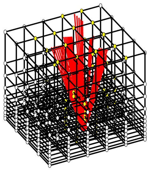
Figure 1.
Global Navigation Satellite System (GNSS) signals (red lines) from single GNSS station for GNSS tomography—the cuboid is the tomographic region adopted in general node parameterization approaches, the yellow solid nodes are those near GNSS signals and the hollow nodes are those in the empty region.
It is common in tomographic modeling that the tomographic region is larger than the region outlined by the GNSS signals. This is because the tomographic region must be extended to cover all of the available GNSS signals at every epoch. For example, Figure 2 shows the trace paths of the signals from one station to multiple GNSS satellites onto the upper boundary at Universal Time Coordinated (UTC) 0 between days of year (DOY) 121, 131, 141 and 151 in 2015. The figure shows that the GNSS signals from orbiting satellites quickly change over time and that the signals are distributed in different directions at different epochs. The figure also shows that over these four days there are empty voxels (empty squares) in which no water vapor parameters need be modelled.
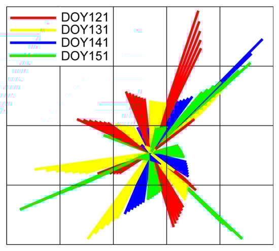
Figure 2.
Top view of the GNSS signals (color radial lines) from one station (in the center of the radial lines) through the top of the tomographic region (pattern grid) at four tomographic epochs.
This highlights that an approach that dynamically determines the single-station tomographic region and its discretization at each tomographic epoch would be beneficial. This new approach (i.e., the HFGT method) would minimize the shape of the irregular tomographic region and would reduce the number of the unknown parameters. This makes the single-station GNSS tomography applied here possible and worth attempting.
2.2. High Flexibility GNSS Tomographic Model
The HFGT approach presented here includes three steps; (1) determination of a tomographic region; (2) determination of node density and position; and (3) estimation of GNSS tomographic parameters. Each of the steps is introduced and described in detail in the following sections. Although GNSS tomography with a single station lacks the observations in most cases, this extreme scheme was also implemented for comparing the quality of the HFGT technique against other schemes.
2.2.1. Determination of a Tomographic Region
In standard tomographic modeling, variable intervals between horizontal planes are often adopted, due to uneven water vapor distribution in the atmosphere (Figure 3a). On each horizontal plane, a Graham scan [24] can be undertaken to identify the convex hull of the intersections between GNSS signals and the plane (the intersection points are named pierce points). This is achieved by utilizing a stack to detect and remove concavities in the boundary efficiently.
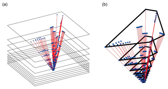
Figure 3.
Determination of the tomographic region; (a) A set of satellite signals (red lines) used in single-station tomographic modeling and their intersections (blue points) with all horizontal planes; (b) Tomographic boundary on every horizontal plane is formed by the black loop obtained based on the Graham scan.
In HFGT, a single-station tomographic region at a given tomographic epoch (Figure 3a) is divided vertically into several horizontal planes with non-uniform vertical intervals from 400 to 3800 m. Pierce points where GNSS signals (red lines) pass through the top of the tomographic model are calculated (blue points in Figure 3). Convex hulls are then defined using the pierce points on each horizontal plane. The resulting boundaries on the plane of interest are called tomographic boundaries (i.e., all the black loops in Figure 3b). The resulting volume enclosing the tomographic region is now irregular in shape and varies from epoch to epoch (e.g., an adaptive approach).
For general node parameterization, the position of water vapor parameters at each node is determined using the cuboid-shaped tomographic region. However, the varied and irregular shaped tomographic region resulting from the new approach (Figure 3b) makes it challenging to select the density of predetermined nodes. Furthermore, due to the limited number of tomographic observations from the single GNSS station, the number of unknown parameters that can be solved must be reduced. To address the above issues, a meshing technique is used to gradually adjust the density and position of nodes for the discretization of the tomographic boundary at each tomographic epoch.
2.2.2. Determination of Node Density and Position
The HFGT technique requires water vapor estimates at uniformly spaced nodes on each horizontal plane. These are generated using the meshing technique described by Ding et al. [19], which is divided into four main steps and illustrated in Figure 4. The first step requires inserting a regularly spaced grid of nodes over each horizontal plane in the tomographic region. Nodes that fall outside of the tomographic boundary (top-right panel) are excluded. Next geometric topologies are considered between the nodes (bottom left panel) resulting in the generation of 2D triangular irregular network on each horizontal plane. A force-displacement algorithm is then iteratively applied to adjust the location of the initial nodes to approximate a regularly sampled grid (bottom-right) according to desired topology criteria. Each step is elaborated in more detail in Ding et al. [19].
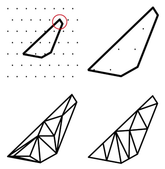
Figure 4.
Rough determination of equidistant nodes by meshing techniques; Top left: background grids (black points) and the shape of the tomographic region (irregular polygon), the shortest edge has been highlighted by the red circle; Top right: initial grids of the tomographic region selected from the background grids; bottom left: a Delaunay triangulation for the initial grids; bottom right: the position of the grids (triangles vertices) moved by the meshing techniques to the roughly equally spaced position.
An undesirable aspect of the HFGT approach is the presence of a ‘shorter’ side around the new tomographic boundary. An example of a short side is highlighted within the red circle in the top-left panel of Figure 4. If this distance is significantly less than the distance between the grid nodes, the choice of the initial grid spacing between nodes becomes very important. In this study, the short side of the tomographic boundary (top left) is first removed before the meshing steps are undertaken. As shown in Figure 5, when this occurs the shape of the boundary can be significantly improved in comparison with that in Figure 4 (bottom left). This provides an improvement in comparison to the position of the original boundary; however some small movements of the nodes near the short boundary are required. It is note that the uniform degree of these nodes largely depends on the shape of the tomographic boundary and the expected distance between the nodes which have the topologies.
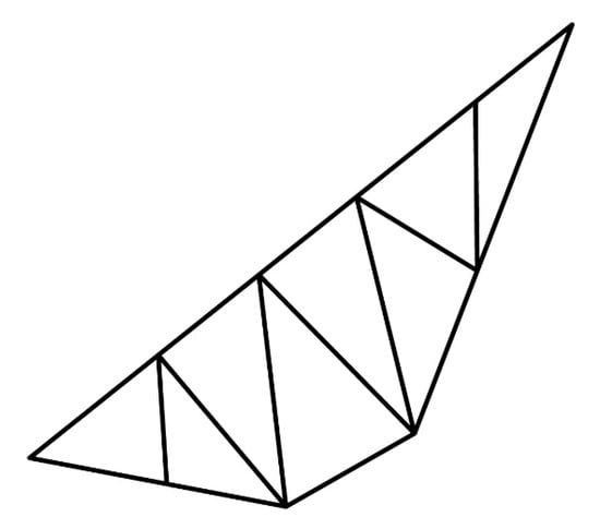
Figure 5.
Adjustment of nodes (triangles vertices) for equidistance without “shorter sides” (The edge surrounded by the red circle in Figure 4).
The dimension of the resulting tomographic boundaries on each horizontal plane will be different (see Figure 3b). As a result, the density of the equally spaced nodes meshed using the procedure described above on each plane will also be different. Given that (1) single station GNSS tomography may result in an insufficient number of tomographic observations, (2) at present, GNSS tomography above 4000 m performs poorly and (3) an imperceptible amount of water vapor exists above 4000 m, the distance between nodes on horizontal planes this elevation is decreased. This inter-node distance is called the expected distance or F0 and can be calculated using the following formula:
where is the expected distance in ith plane; Ci is a constant coefficient in ith plane which is used to adjust the value of F0 in different planes and mean value () is the mean of the perimeter lengths of the polygon of the boundary in ith plane. The value of constant coefficient Ci is 0.45 when the height of plane is less than or equal to 4000 m and 0.75 when the height is above 4000 m. After removing the ‘shorter sides’ and applying the meshing techniques with F0, all the nodes are then adjusted from the initial position to an equidistant position on each plane (e.g., Figure 6 (top panel)) and these modified nodes are called the tomographic nodes.
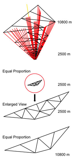
Figure 6.
Distribution of GNSS signals at each tomographic plane; top panel: all the nodes (triangles vertices) are adjusted to an equidistant position on each plane; middle panel: equal proportion and enlarged view of the nodes at the height of 2500 m; bottom panel: equal proportion of the nodes at the height of 10,800 m.
The results show that the density of the tomographic nodes below or equal to 4000 m height (e.g., the nodes at the height of 2500 m in middle panel) are greater than that of nodes above 4000 m (e.g., the nodes at the height of 10,800 m in bottom panel). Also, removing the short leads to some GNSS signals outside of the tomographic region (e.g., GNSS signal (yellow line) in top panel). These signals can also be used to build observation equations for parameter estimates in GNSS tomography.
2.2.3. Estimation of GNSS Tomographic Parameters
Following the above steps, an integro-interpolation algorithm [10] is used to build observation equations and to estimate water vapor density (or SWV) at each tomographic node. The value of SWVs can be expressed as the water vapor densities at the corresponding tomographic nodes. Therefore, GNSS tomographic observation equations can be constructed as
where A is the coefficient matrix of the tomographic model; b represents the vector of SWV observations; and X is the vector of the water vapor density at all the tomographic nodes. The access order scheme based on prime number decomposition (PND) proposed in Ding et al. [25] is used for solving the unknowns in Equation (3).
3. Results
The HFGT modeling approach was tested with non-uniform vertical layers. Raw data from the Hong Kong Satellite Positioning Reference Station Network (SatRef) are used to validate the new approach. In this study, due to multi-group tests need to use the GNSS stations from the SatRef repeatedly, the name of the GNSS stations are replaced by serial numbers for convenience. The corresponding number and horizontal position of the GNSS stations in the test area are shown in Figure 7. The height range of the area is 0–10,800 m. Radiosonde data from the King’s Park Meteorological Station (HKKP) are used as a reference to compare against the moisture profiles derived from the GNSS tomographic model. GNSS data between DOY 121 to 151 were processed with GAMIT software. For atmospheric delay models of GAMIT, the Saastamoinen model was set as the expressions for the dry zenith delay and the VMF1 mapping function was used for both the hydrostatic and wet delay.
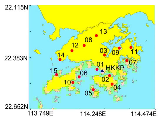
Figure 7.
The horizontal distribution of the GNSS stations (red dots), King’s Park Meteorological Station (HKKP) (blue triangle)—the ground observation station and the tomographic area for GNSS tomography.
3.1. GNSS Tomographic Schemes
To validate the performance of the HFGT, fifteen GNSS tomographic schemes were implemented according to the distance and orientation between King’s Park Meteorological Station (HKKP) and GNSS stations. We name all schemes according to the GNSS tomographic approach, a hyphen and the last station number. Scheme HFGT-01 takes into consideration station 01, scheme HFGT-02 takes into consideration station 01 and 02 and subsequently. For examples, HFGT-09 means the HFGT is used to modeling the 3D water vapor field based on the GNSS data from station 01 to station 09. It is note that GNSS stations which used in the schemes are defined by the initial station number (i.e., number 01) and the last station number. Since all schemes have the same initial station number, it did not appear in the scheme name.
The GNSS tomographic schemes are designed to verify the accuracy and reliability of the HFGT for different size of the GNSS network. The single station (i.e., HFGT-01) or the double station (i.e., HFGT-02) for the innovative approach is an extreme case to research on the relationship between the increase of the GNSS station (tomographic observation) and the tomographic results.
3.2. Validation of the HFGT
Root-mean-square error (RMSE) statistics are calculated daily at UTC 12 for the whole month of data for the HFGT modeling results. The results of the fifteen schemes are shown in Figure 8 and for simplification, the last station number as part of the scheme name instead of the full scheme name. Figure 8 shows the best result occurs in the HFGT-08; while the worst result occurs in the HFGT-02. In fact, the schemes which the last station numbers less than three have a poor performance in comparison with the other schemes. The results suggest that the small number of the GNSS stations lack essential observations for GNSS tomography. As the number of stations increases, the results of the schemes achieve a better level of accuracy with slight fluctuations. However, the best result is not as expected occurs in the HFGT-15, that is, we cannot simply come to the conclusion that the more stations, the higher the accuracy. The GNSS stations which far away from the HKKP in fact does little contribution to the improvement on the tomographic result at the HKKP. Therefore if we want to achieve higher accuracy of the tomographic results, the correlation between the tomographic inversion region and the observations that from GNSS stations is necessary to be considered.
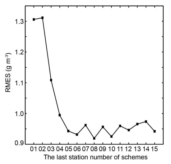
Figure 8.
Root-mean-square error (RMSE) (black squares) of the fifteen GNSS tomographic schemes in the 31-day period; HKKP’s radiosonde data were used as the reference.
The distribution of the GNSS signals is another important factor which significantly impacts the tomographic results. As an example, the daily tomographic solutions of the HFGT-01 are compared against moisture profiles derived from the HKKP to analyze the relationship between the distribution of the GNSS signals and the accuracy of the tomographic solutions. The results are shown in Figure 9. The best result occurs on DOY 126; while the worst result occurs on DOY 146.
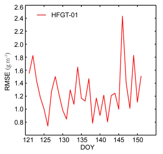
Figure 9.
RMSE (red line) of HFGT-01 at Universal Time Coordinated (UTC) 12 in the 31-day period; HKKP’s radiosonde data were used as the reference.
To investigate these two results (e.g., on DOY 126 and 146), the tomographic area, tomographic geometry of the GNSS signals in the model domain on these days are considered and shown in Figure 10. The figure shows that in 3D, the distributions of the GNSS signals on both days are similar. However, when viewed from the right-hand side, the figure shows that the best result (top) has a uniform distribution of GNSS signals in the tomographic region, while the worst result (bottom) occurs when this distribution is uneven. In this instance lower elevation signals have extended the tomographic area and their lower density may have resulted in poor quality estimates at the nodes in this vicinity. Further, these low-elevation signals and their low density have likely decreased the overall quality of the tomographic results. Other schemes which have a low number are obviously influenced by the distribution of the GNSS signals since these schemes often lack necessary GNSS observations. As the number of the GNSS stations increase, this problem is improved by the high-density GNSS signals (i.e., sufficient observations).
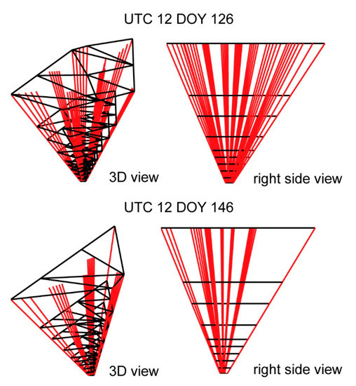
Figure 10.
The tomographic area (all black loops), tomographic nodes (triangles vertices) and distribution of GNSS signals (red lines) at UTC 12 on DOY 126 (top) and DOY 146 (bottom).
To further explore this influence, water vapor profiles obtained from the HFGT technique were compared against the radiosonde data at UTC 12 on DOY 126 and 146 (see Figure 11). The figure shows that a strong correlation is present between the two profiles for DOY 126 but for DOY 146, a weaker correlation exists, specifically in two intervals (i.e., between heights of 1000 m and 2000 m and that of 4500 m and 6500 m), where a significant difference is observed. The results suggest that the even distribution of the GNSS signals and sufficient observations significantly impacts the tomographic results.
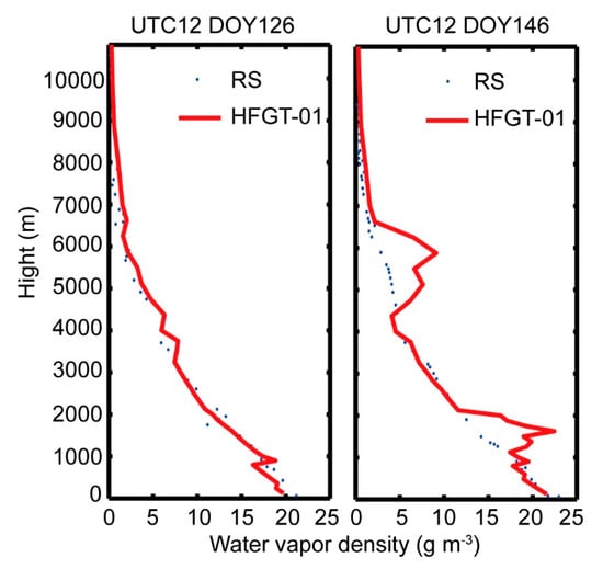
Figure 11.
Water vapor profiles (red curves) obtained from HFGT-01 compare against that of radiosonde data (RS) (blue points) on DOY 126 and DOY 146.
The RMSE, bias, standard deviation, correlation coefficient, inter-quartile range (IQR) and outlier from the results of the new approach in the 31-day period are shown in Table 1 and the minimum values of these statistics present in HFGT-08, HFGT-10 and HFGT-06. All three schemes contain a sufficient number of GNSS stations and a strong correlation with the HKKP. On the other hand, the worst result of the statistics present in HFGT-01 and HFGT-02. The RMSE obtained by the HFGT-08 is roughly 30% smaller by compared to the HFGT-01 and HFGT-02. The correlation coefficient of HFGT-08 presents the strongest possible agreement among all the schemes. HFGT-08 also has a relatively small Bias to be consistent with this strong correlation. However, the standard deviation of HFGT-08 seems that the estimates of the water vapor are spread out over a wider range. It is noted that the water vapor in the troposphere exponentially decreases with the increase of height, which indicates that the estimates of the water vapor will not tend to be close to the mean (i.e., large standard deviations occur in all schemes or the amount of variation of the water vapor is great). The differences of IQR between schemes are not obvious in comparison with that of the RMSE but the values of outliers that are derived by IQRs also reflect the performance of all schemes. The schemes with the last number that less than three have the larger value of outliers, indicating that insufficient observations result in the low stability for the tomographic modeling.

Table 1.
Monthly statistics of the The High Flexibility GNSS Tomography (HFGT) results (radiosonde data (RS) from the King’s Park Meteorological Station (HKKP) was used as the reference).
In the previous analysis, the statistics from the results of the new approach in the 31-day period are analyzed for comparing the difference of schemes. In this paragraph, GNSS tomographic region-related parameters in the 31-day period have been introduced in Table 2 to quantify the impact of the tomographic region. It should be noted that all these four parameters are mean values in the 31-day. The size of the top tomographic region (i.e., top region in Table 2) and the “diffusion coefficient” which defined by the ratio of the size of the top tomographic region to that of the bottom are the main factors for the analysis of the tomographic region. The mean altitudinal angle of the GNSS signals and the number of signals used in each scheme are focus on the correlation between the tomographic region and observations. All region-related parameters are increased as the last number of schemes increase except the diffusion coefficient. The diffusion coefficient greater than about twenty following a relatively poor quality of the tomographic region, which refers to the poor monthly statistics of the HFGT results in Table 1. When the diffusion coefficient below about 10, the quality of the tomographic region fluctuates in a specific range. Although the GNSS tomographic region was enlarged with rising number of signals, the mean altitudinal angle changes a little in each scheme. The results suggest that the observations for tomographic modeling in a small area like Hong Kong mostly have a fixed range of altitudinal angles. Besides, the tomographic observations have large altitudinal angles.
Table 2.
Mean monthly of the GNSS tomographic region-related parameters.
In this paragraph, we focus on the results of all the schemes on DOY 146, since the worst result of the HFGT-01 occurs on DOY 146 (i.e., 2.430 (g m−3) during these 31 days (in Figure 9). As shown in Figure 12, the results of the GNSS tomography are significantly improved with the increase of the number of schemes. The best result is achieved in the HFGT-07 (i.e., 0.499 (g m−3))—that’s almost a five-fold increase comparison with the HFGT-01. To offer a more intuitionistic comparison, in Figure 13, water vapor profiles obtained from the HFGT-01 and HFGT-07 were compared against the radiosonde data on DOY 146. This is similar to the results of the HFGT-01 in the 31-day period (in Figure 9)—the results of the schemes achieve a better level of accuracy with the increase of the GNSS stations on DOY 146 but the best result still not occurs in the scheme which has the maximum number of the stations. The results are shown in Figure 9 and Figure 12, which indicate that the accuracy of the tomographic result is significantly influenced by the number of observations (from GNSS station), the distribution of the GNSS signals and the correlation between the tomographic region and the observations.
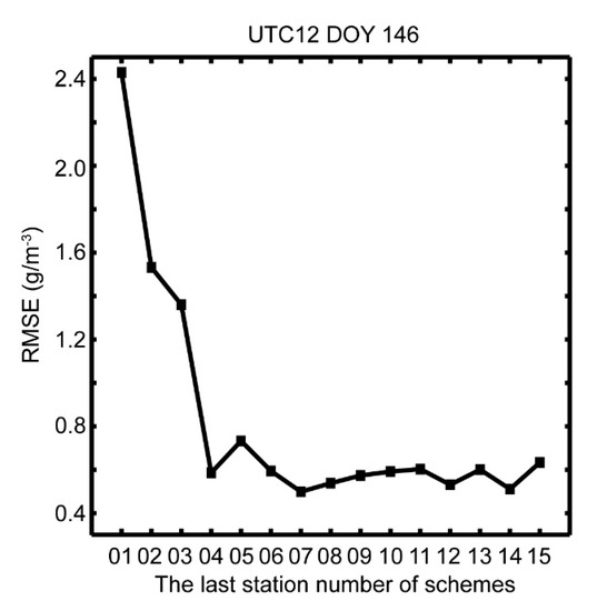
Figure 12.
RMSE (black squares) of the fifteen GNSS tomographic schemes at UTC 12 on days of year (DOY) 146; HKKP’s radiosonde data were used as the reference.
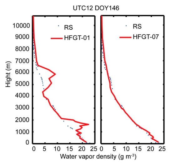
Figure 13.
Water vapor profiles (red curves) obtained from HFGT-01 and HFGT-07 were compared against that of RS (blue points) on DOY 146.
4. Conclusions
A new approach to High Flexibility GNSS Tomography is proposed in this study. With this approach, the Graham scan method is used to discretize the tomographic region by finding the convex hulls (tomographic boundaries) of the pierce points between the paths of all GNSS signals and the tomographic planes at different heights. After that, the shape of each tomographic boundary is adjusted by removing the “shorter sides” to ensure the high geometrical quality of tomographic nodes (i.e., nodes are as close to evenly distributed as possibly at different heights of tomographic boundaries). After the above procedures are applied to determine the discrete tomographic region, meshing techniques are adopted to define the density and the positions of nodes on all tomographic planes at each tomographic epoch. Considering the fact that the present GNSS tomography method above 4000 m has a poor performance and little water vapor exists in that area, the number of tomographic nodes above 4000 m is decreased by increasing the expected distance to avoid too many unknown parameters to be calculated. Instead of a pre-set regular and fixed tomographic region used in traditional GNSS tomography for all tomographic epochs, the new approach reduces a large number of redundant parameters. This leads to GNSS tomography by any size of the GNSS network can be implemented.
The new approach (i.e., HFGT) was tested and its performance was compared with the radiosonde data from HKKP in May 2015. HFGT is tested by fifteen GNSS stations from the SatRef. The RS data at UTC 12 from HKKP are used for the validation of the performance of HFGT. Monthly statistics of the HFGT and single day results from fifteen schemes indicated that the new approach is feasible for any size of the GNSS network, even for the few GNSS stations when the sufficient and uniformed signals are used for GNSS tomography. It is unfortunate that the new approach has a poor performance in the tomographic region which the GNSS signals are unevenly covered. However, it is noted that uneven coverage does not necessarily mean lack of the GNSS signals, it could be due to an “oversized” tomographic region caused by the low-angle GNSS signals by including too many parameters to be solved. Fortunately, the uneven distributions of the GNSS signals, in most cases, occur in the schemes, which the last station number of the schemes below three. Also, the results indicated that the number of observations (from GNSS stations), the distribution of the GNSS signals and the correlation between the tomographic region and the observations significantly impact the accuracy of the tomographic results. The diffusion coefficient (in Table 2) partly reflects the quality of the tomographic region and it also reveals the impacts of the distribution of observations to the tomographic region. The small diffusion coefficient means that there is not much difference between the top and the bottom of the GNSS tomographic region or in other words, the distribution of the observations is suited for the GNSS tomographic modeling. In small areas (e.g., Hong Kong), the data of the GNSS signals which has large altitudinal angles make up the majority of the tomographic observations and the tomographic region.
In the future, the work will focus on using the multi-system satellites, for example, GPS, GLONASS and BDS system, to increase the tomographic observations, which is extremely important for GNSS tomography.
Author Contributions
Conceptualization, N.D. and Y.W.; methodology, N.D.; software, Y.W.; validation, Y.Z. and L.L.; formal analysis, Y.Z. and L.L.; writing—original draft preparation, Y.W. and N.D.; writing—review and editing, X.Y. and Q.Z.; funding acquisition, N.D. and X.Y. All authors have read and agreed to the published version of the manuscript.
Funding
This research was funded by the National Natural Science Foundation of China, grant number 41904013; the National Natural Science Foundation of China, grant number 41601087; the Priority Academic Program Development of Jiangsu Higher Education Institutions (PAPD).
Acknowledgments
The authors acknowledge the Survey and Mapping Office (SMO) of Lands Department, Hong Kong for the provision of GNSS data from the Hong Kong Satellite Positioning Reference Station Network (SatRef). We also thank King’s Park Observatory for the provision of radiosonde data and the Department of Earth Atmospheric and Planetary Sciences, MIT for the GAMIT/GLOBK software. The editor and reviewer team is also highly appreciated for their valuable comments, which makes great improvements in the quality of the paper.
Conflicts of Interest
The authors declare no conflict of interest.
References
- Zhao, Q.; Yao, Y.; Yao, W. Troposphere Water Vapour Tomography: A Horizontal Parameterised Approach. Remote Sens. 2018, 10, 1241. [Google Scholar] [CrossRef]
- Flores, A.; Ruffini, G.; Rius, A. 4D tropospheric tomography using GPS slant wet delays. Ann. Geophys. 2000, 18, 223–234. [Google Scholar] [CrossRef]
- Hirahara, K. Local GPS tropospheric tomography. Earth Planets Sp. 2000, 52, 935–939. [Google Scholar] [CrossRef]
- Xia, P.; Cai, C.; Liu, Z. GNSS troposphere tomography based on two-step reconstructions using GPS observations and COSMIC profiles. Ann. Geophys. 2013, 31, 1805–1815. [Google Scholar] [CrossRef]
- Chen, B.; Liu, Z. Voxel-optimized regional water vapor tomography and comparison with radiosonde and numerical weather model. J. Geod. 2014, 88, 691–703. [Google Scholar] [CrossRef]
- Jiang, P.; Ye, S.R.; Liu, Y.Y.; Zhang, J.J.; Xia, P.F. Near real-time water vapor tomography using ground-based GPS and meteorological data: Long-term experiment in Hong Kong. Ann. Geophys. 2014, 32, 911–923. [Google Scholar] [CrossRef]
- Rohm, W.; Zhang, K.; Bosy, J. Limited constraint, robust Kalman filtering for GNSS troposphere tomography. Atmos. Meas. Tech. 2014, 7, 1475–1486. [Google Scholar] [CrossRef]
- Yao, Y.B.; Zhao, Q.Z.; Zhang, B. A method to improve the utilization of GNSS observation for water vapor tomography. Ann. Geophys. 2016, 34, 143–152. [Google Scholar] [CrossRef]
- Ye, S.; Xia, P.; Cai, C. Optimization of GPS water vapor tomography technique with radiosonde and COSMIC historical data. Ann. Geophys. 2016, 34, 789–799. [Google Scholar] [CrossRef]
- Ding, N.; Zhang, S.; Wu, S.; Wang, X.; Kealy, A.; Zhang, K. A new approach for GNSS tomography from a few GNSS stations. Atmos. Meas. Tech. 2018, 11, 3511–3522. [Google Scholar] [CrossRef]
- Seko, H.; Shimada, S.; Nakamura, H.; Kato, T. Three-dimensional distribution of water vapor estimated from tropospheric delay of GPS data in a mesoscale precipitation system of the Baiu front. Earth Planets Sp. 2000, 52, 927–933. [Google Scholar] [CrossRef]
- Shrestha, S.M. Investigations into the Estimation of Tropospheric Delay and Wet Refractivity Using GPS Measurements; Department of Geomatics Engineering, University of Calgary: Calgary, AB, Canada, 2003. [Google Scholar]
- Gradinarsky, L.P.; Jarlemark, P. Ground-Based GPS Tomography of Water Vapor: Analysis of Simulated and Real Data. J. Meteorol. Soc. Jpn. 2004, 82, 551–560. [Google Scholar] [CrossRef][Green Version]
- Troller, M.R. GPS Based Determination of the Integrated and Spatially Distributed Water Vapor in the Troposphere. Ph.D. Thesis, Eidgenössische Technische Hochschule Zürich, Zürich, Switzerland, 2004. [Google Scholar]
- Hoyle, V.A. Data Assimilation for 4-D Wet Refractivity Modelling in a Regional GPS Network; University of Calgary: Calgary, AB, Canada, 2005. [Google Scholar]
- Bender, M.; Dick, G.; Wickert, J.; Ramatschi, M.; Ge, M.; Gendt, G.; Rothacher, M.; Raabe, A.; Tetzlaff, G. Estimates of the information provided by GPS slant data observed in Germany regarding tomographic applications. J. Geophys. Res. 2009, 114, D06303. [Google Scholar] [CrossRef]
- Donat Perler Water Vapor Tomography Using Global Navigation Satellite Systems; Eidgenössische Technische Hochschule Zürich: Zürich, Switzerland, 2011.
- Shangguan, M.; Bender, M.; Ramatschi, M.; Dick, G.; Wickert, J.; Raabe, A.; Galas, R. GPS tomography: Validation of reconstructed 3-D humidity fields with radiosonde profiles. Ann. Geophys. 2013, 31, 1491–1505. [Google Scholar] [CrossRef]
- Ding, N.; Zhang, S.B.; Wu, S.Q.; Wang, X.M.; Zhang, K.F. Adaptive Node Parameterization for Dynamic Determination of Boundaries and Nodes of GNSS Tomographic Models. J. Geophys. Res. Atmos. 2018, 123, 1990–2003. [Google Scholar] [CrossRef]
- Askne, J.; Nordius, H. Estimation of tropospheric delay for microwaves from surface weather data. Radio Sci. 1987, 22, 379–386. [Google Scholar] [CrossRef]
- Wang, X.; Zhang, K.; Wu, S.; Fan, S.; Cheng, Y. Water vapor-weighted mean temperature and its impact on the determination of precipitable water vapor and its linear trend. J. Geophys. Res. Atmos. 2016, 121, 833–852. [Google Scholar] [CrossRef]
- Shoji, Y.; Nakamura, H.; Iwabuchi, T.; Aonashi, K.; Seko, H.; Mishima, K.; Itagaki, A.; Ichikawa, R.; Ohtani, R. Tsukuba GPS Dense Net Campaign Observation: Improvement in GPS Analysis of Slant Path Delay by Stacking One-way Postfit Phase Residuals. J. Meteorol. Soc. Jpn. 2004, 82, 301–314. [Google Scholar] [CrossRef]
- Kačmařík, M.; Douša, J.; Dick, G.; Zus, F.; Brenot, H.; Möller, G.; Pottiaux, E.; Kapłon, J.; Hordyniec, P.; Václavovic, P.; et al. Inter-technique validation of tropospheric slant total delays. Atmos. Meas. Tech. 2017, 10, 2183–2208. [Google Scholar] [CrossRef]
- Graham, R.L. An efficient algorith for determining the convex hull of a finite planar set. Inf. Process. Lett. 1972, 1, 132–133. [Google Scholar] [CrossRef]
- Ding, N.; Zhang, S.; Zhang, Q. New parameterized model for GPS water vapor tomography. Ann. Geophys. 2017, 35, 311–323. [Google Scholar] [CrossRef]


© 2020 by the authors. Licensee MDPI, Basel, Switzerland. This article is an open access article distributed under the terms and conditions of the Creative Commons Attribution (CC BY) license (http://creativecommons.org/licenses/by/4.0/).