Abstract
Ground-penetrating radar (GPR) is a convenient geophysical technique for active-layer soil moisture detection in permafrost regions, which is theoretically based on the petrophysical relationship between soil moisture (θ) and the soil dielectric constant (ε). The θ–ε relationship varies with soil type and thus must be calibrated for a specific region or soil type. At present, there is lack of such a relationship for active-layer soil moisture estimation for the Qinghai–Tibet plateau permafrost regions. In this paper, we utilize the Complex Refractive Index Model to establish such a calibration equation that is suitable for active-layer soil moisture estimation with GPR velocity. Based on the relationship between liquid water, temperature, and salinity, the soil water dielectric constant was determined, which varied from 84 to 88, with an average value of 86 within the active layer for our research regions. Based on the calculated soil-water dielectric constant variation range, and the exponent value range within the Complex Refractive Index Model, the exponent value was determined as 0.26 with our field-investigated active-layer soil moisture and dielectric data set. By neglecting the influence of the soil matrix dielectric constant and soil porosity variations on soil moisture estimation at the regional scale, a simple active-layer soil moisture calibration curve, named CRIM, which is suitable for the Qinghai–Tibet plateau permafrost regions, was established. The main shortage of the CRIM calibration equation is that its calculated soil-moisture error will gradually increase with a decreasing GPR velocity and an increasing GPR velocity interpretation error. To avoid this shortage, a direct linear fitting calibration equation, named as υ-fitting, was acquired based on the statistical relationship between the active-layer soil moisture and GPR velocity with our field-investigated data set. When the GPR velocity interpretation error is within ±0.004 m/ns, the maximum moisture error calculated by CRIM is within 0.08 m3/m3. While when the GPR velocity interpretation error is larger than ±0.004 m/ns, a piecewise formula calculation method, combined with the υ-fitting equation when the GPR velocity is lower than 0.07 m/ns and the CRIM equation when the GPR velocity is larger than 0.07 m/ns, was recommended for the active-layer moisture estimation with GPR detection in the Qinghai–Tibet plateau permafrost regions.
1. Introduction
Soil moisture information is essential for understanding permafrost regions’ environmental evolution, such as active-layer freezing and thawing processes and its special distribution modelling. The active layer is defined as the layer of ground that is subject to seasonal thawing and freezing in areas underlain by permafrost. It plays a vital role in hydrological processes, heat flux exchanges between ground and air, as well as land surface modeling. Moreover, it can also affect carbon cycles, terrestrial ecosystems, and permafrost region ground engineering. The principal factors which influence the spatial variation of active-layer thickness are ground surface soil temperature, soil moisture, and thermal conductivity within the active layer. In fact, soil temperature and thermal conductivity are also affected or directly controlled by soil moisture. Soil moisture monitoring or acquisition in field work is essential for active-layer spatial distribution investigation and modelling. At present, active-layer soil moisture was often monitored with the buried time domain reflectometry (TDR) [1] sensor or acquired through traditional gravimetric methods with active-layer profile soil samples. These in situ measurements may be prone to uncertainties due to, for example, loss of intimate contact between sensors and the surrounding soil because of shrinkage or biological activity, or a lack of calibration, especially for soils with high specific surface areas. In addition, implementation of such methods is destructive, expensive, and laborious and they only provide localized information about active-layer soil moisture. Because of the high spatial variability of soil moisture due to spatiotemporal variations of associated meteorological and biogeophysical parameters, measurement and monitoring of large-scale active-layer soil moisture is challenging.
Ground-penetrating radar (GPR) is one of the most convenient geophysical techniques to detect soil moisture at catchment scales and can be used for high-resolution subsurface moisture distribution investigations at the centimeter-scale resolution. In permafrost regions, the seasonal thawing/frozen interface between the active layer and permafrost layer provides a very good condition for GPR detection of active-layer thickness distribution. Utilizing the GPR signal traveling speed within the active layer, the bulk dielectric constant of the active-layer soil profile can be theoretically calculated, and then soil moisture can be estimated through empirical calibration equations based on the relationship between the soil dielectric constant and its volumetric water content. A comprehensive review of methods to acquire soil water content with GPR were provided by Huisman [2], who pointed out that GPR can be used by experienced researchers to provide reliable estimates of subsurface water content. Parsekian [3] have confirmed through calibration that GPR is an effective tool for investigating water content in peat soil and can produce accurate results that are comparable with TDR measurements. Active-layer soil moisture estimation based on GPR detection was often applied in arctic permafrost regions, such as active-layer thickness investigation [4], seasonal frost heave and thaw settlement calculation [5], as well as validation of Low-Frequency SAR soil moisture modelling [6]. At present, there are seldomly research on the applicability or accuracy estimation of GPR detection specific for active-layer soil moisture, especially not in the Qinghai–Tibet permafrost regions.
The most important issue of active-layer soil moisture acquisition with GPR is the petrophysical relationship between permittivity and volumetric water content, which needs further accurate evaluation or calibration for researched soil types. All the soil permittivity–moisture relationship models can be classified into two categories. The first type is empirical polynomial fit equations that were based on laboratory tests for specific soil types, such as sand, silt, clay, peat, mineral soil with different organic content, and so on. As far as we know, Topp [7] and Roth [8] had conducted very excellent laboratory experiments with TDR for different soil types, and had provided a series of empirical fit equations suitable for different soil types. Many empirical fit equations were also provided by commercial TDR probe sensor providers, e.g., equations of sand, silt, and clay for the Hydra probe from Stevens Water Monitoring Systems, Inc. (www.stevenswater.com). The major flaw of these polynomial fit equations is that they cannot be used for the extrapolation calculation of soil water content. When the measured soil water content is larger than the largest water content of the original tested soil samples, in other words, the measured dielectric constant of a different soil sample is larger than the largest permittivity of the original tested soil sample that is used for the establishment of the polynomial fit equation, then the calculated volumetric soil water content may have large errors or exceed 1 m3/m3. For example, a polynomial calibration fit equation was acquired by Zamolodchikov [9] in the Russian Far East tundra region, utilizing a Vitel portable probe with 185 volumetric soil samples taken from different ecosystems and organic/mineral horizons with varying moisture content. When this calibration curve was applied in the Alaskan Arctic coastal plain near Barrow, in a similar ecosystem, tundra, at least a 20% calculated error existed for the soil samples tested by Engstrom [10]. The active layer, often appearing as a compound regolith composed of vegetation, organic material, accumulated mineral horizon, and weathered parent material, cannot simply be classified as certain determined soil types due to its large variation in spatial scale. So, the laboratory-tested calibration curves cannot be directly applied for active-layer soil moisture calculation.
The second type is the Complex Refractive Index Model, which is a physical soil model. In this model, the bulk dielectric constant of a soil–water–air system, ε, can be expressed in the following form suggested by Huisman [2]:
where θ is the soil water content (m3/m3); φ is the soil porosity (m3/m3); εw, εs, and εa represent the dielectric constant of soil water, solid soil part, and air (εa = 1), respectively; and n is a factor accounting for the orientation of the electrical field with respect to the geometry of the soil medium (n = 1 for an electrical field parallel to soil layers, n = −1 for an electrical field perpendicular to soil layers, and n = 0.5 for an isotropic soil layer). Birchak et al. [11] found n = 0.5 for an isotropic two-phase medium from travel time calculations for electromagnetic waves. Based on this result, the default number value of n = 0.5 was accepted by many researchers for three- or four-phase soil mixtures [2,12,13]. In order to obtain the best estimation of gas content in peat, a = 1 was used by Comas [14]. Parsekian’s experiment showed that n = 0.1, 0.28, 0.33, or 0.36 have the best fitting for four different peats, respectively [3]. Dobson et al. [15] determined n by regression from data for different frequencies (1.4—18 GHz) and soil types (ranging from sandy loam to silty clay) and obtained n = 0.65. The parameter n in Equation (1) was often considered as an experienced number and needs to be calibrated for different soil types.
In order to acquire a more accurate calibration equation that is suitable for active-layer soil moisture estimation with GPR velocity, a simplified Complex Refractive Index Model and a direct linear fitting equation with GPR velocity and soil moisture were established, respectively, based on a field-investigated active-layer soil moisture and corresponding GPR velocity data set from the Qinghai–Tibet plateau permafrost regions. In Section 2, our field investigation of active-layer pits for real soil moisture and the GPR survey methods are described. At the same time, the possible GPR velocity interpretation error, which will influence active-layer soil moisture estimation accuracy and the selection of calibration equations, was indirectly provided through the comparison of different GPR detection methods. In Section 3, one main parameter within the Complex Refractive Index Model, the dielectric constant of the soil water within the active layer was firstly calculated based on the relationship between the water dielectric constant and temperature and salinity. Then the second main parameter, exponent number, was deduced utilizing the calculated soil water dielectric constants and the linear fitting slopes of the field-investigated active-layer soil moisture and dielectric constant data set under different exponential case from −1 to 1. Finally, a simplified Complex Refractive Index Model, named CRIM, was acquired through neglecting the influence of the soil matrix dielectric constant and porosity variations on moisture estimation at the regional scale. In the subsection of error analysis, the calculated soil-moisture error with CRIM under different GPR velocity interpretation error cases was analyzed. Subsequently, based on the statistical relationship between the active-layer soil moisture and GPR velocity, we recommended a direct linear fitting calibration equation, named υ-fitting, which can be used to reduce the moisture calculation error when GPR velocity is lower than 0.07 m/ns. Essentially, both calibration equations of CRIM and υ-fitting were constructed based on field measurements and detected active-layer sample data. In order to evaluate their applicability to the Qinghai–Tibet plateau permafrost regions, the representativeness of our active-layer sample data were analyzed with two factors, soil bulk density and organic content, in Section 4. Section 5 is the discussion, in which the applicability of the CRIM and υ-fitting equations in our research regions are discussed in detail. In Section 6 we conclude this study.
2. Field Investigation Methods and Data
2.1. Active-layer Pits Investigation and Data
Soil pits were excavated to the permafrost layer or seasonal thawing interface. The soil samples were collected from depths in the range of 0–10 cm, 10–20 cm, 20–30 cm, 30–50 cm, 70–100 cm, and within 100 cm depths, and collected at every 50 cm when depth exceeded 100 cm. Within each depth range, three evenly distributed soil samples were collected. The standard cutting-ring method and oven drying were applied for measurements of soil water content and dry bulk density. In addition, as part of our GPR detecting points, the serial number (SN) had the initial letter “R”, and soil organic content was tested and calculated with the K2Cr2O7-H2SO4 method in the laboratory [16]. Living parts (e.g., roots) were picked out before organic matter was tested; so, the actual total organic contents may be higher than the tested results. In this paper, the weighted depth average of dry soil bulk density (ρ_g/cm3), volumetric water content (θ_measured), and soil organic matter content (mass percent, SOM_%) were calculated and we considered the calculated volumetric water content as the true active-layer soil water content. The land-cover types (LandCover) were defined by dominant species and drainage conditions. All the above parameters are presented in Table 1, within which the soil pits’ excavating time (Time), active layer depths uncovered by pits (ALD_m), and depth type (DepthType) are also presented. In general, seasonal thawing depth will reach its annual maximum thawing depth in September or October in the Qinghai–Tibet plateau permafrost regions, which can be considered as the active layer depth (ALD). Depth acquired before this time, for example in July or August of our field work, the active layer depths were considered as the seasonal thawing depth (STD). In addition, the corresponding active-layer dielectric constants (ε) calculated by GPR velocity from the pit profile calibration is also shown in Table 1.

Table 1.
Active-layer soil water content investigation data table.
2.2. GPR Survey and Data Analysis
Ground-penetrating radar (GPR) is now a well-accepted geophysical technique for detecting active-layer thickness or its thawing depth in permafrost regions. The electromagnetic wave transmitted by GPR transmitting antenna will reflect back at the frozen–thawed interface and then be received by the receiving antenna (Figure 1a). In general, a high energy reflecting wave signal at the frozen–thawed interface corresponding to a certain travel time can be recognized on a common offset GPR image (Figure 1b). In order to acquire depth information, radar wave velocity within the active layer must be obtained. In our field work, three velocity detecting methods were applied: (1) wide angle reflection and refraction; (2) multi-offset soundings; and (3) pit profile calibration. In our field GPR detection, a MALÅ ProEx GPR system (Malå Co., Sweden) was applied. A pair of 100 MHz unshielded antennae was used. All the GPR images were interpreted under human–computer interaction with Reflexw software (www.sandmeier-geo.de).
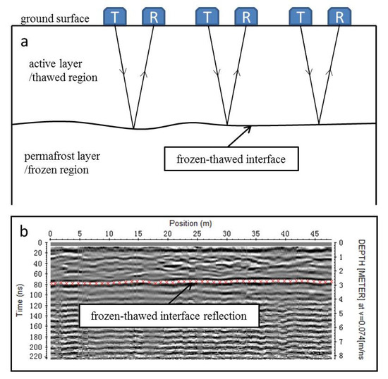
Figure 1.
(a) Schematic diagram of active layer detecting with ground-penetrating radar (GPR); (b) real GPR profile data with the interpreted frozen–thawed interface reflection.
In wide-angle reflection and refraction (WARR) detecting, the transmitting antenna stays fixed and the receiving antenna is moved at fixed steps along a measuring tape, or vice versa. In our field work, the unfixed antenna was manually moved step-by-step with a 0.1 m step length. There is a great possibility for inaccurate antenna placing due to inadvertence from the antenna holder, which will give rise to inaccurate GPR velocity fitting results and cannot be recognized easily with a traditional WARR profile. For accurate reflecting signal recognizing (i.e., the direct ground wave, reflecting wave at the frozen–thawed interface, and other noise signals) and velocity interpreting, a modified WARR detecting was applied in our field work, which is temporally named as back–forward wide-angle reflection and refraction (BFWARR). In the BFWARR detecting, transmitting and receiving antennas are firstly placed with maximum antenna separation (7 m in our field work), with one antenna staying fixed and the other antenna is moved step-by-step with a fixed step length (0.1 m in our field work) till the two antennas come together with a 0 m antenna separation; then back forward to its beginning position (Figure 2a). Both WARR and BFWARR detections require that the soil interface reflection is flat. So, the general location of BFWARR detection was selected from the pre-acquired common offset GPR profile. The BFWARR GPR profile can be divided into two parts. The first part (e.g., 0–14 m in Figure 2b) was acquired with the transmitting antenna (or receiving antenna) fixed; the second part (e.g., 14–28 m in Figure 2b) was acquired with the receiving antenna (or transmitting antenna) fixed. If the two parts of BFWARR GPR profile have the same interpreted velocity, we believed that the active-layer soil moisture distributes evenly in the lateral direction within the BFWARR detection coverage. Then, at the mid-point of the detection coverage, an active layer pit was dug to acquire soil samples for active-layer soil moisture measurement. We used this GPR velocity detection method to determine the best pit excavation position during field work. Each part can also be divided into two sub half parts. The first sub-part halves (e.g., 0–7 m and 14–21 m in Figure 2b) were acquired with the unfixed antenna moving toward to the fixed antenna; the second sub-part halves (e.g., 7–14 m and 21–28 m in Figure 2b) were acquired with the unfixed antenna moving away from the fixed antenna. Within each part, if the first half and second half profile are quasi symmetric, it can be believed that the antenna holder had accurately moved the antenna during the detection process. If not, the BFWARR detection will be repeated again. On the BFWARR profile, direct air wave and direct ground wave appear as mirror-symmetric oblique straight lines with different absolute slopes, which are corresponding to their respective velocities; reflecting waves at the frozen–thawed interface appears as standard hyperbola and its velocity can be calculated or easily acquired through parabolic curve fitting.

Figure 2.
(a) Schematic diagram of back–forward wide-angle reflection and refraction (BFWARR) detection; (b) real BFWARR detection GPR data and the identified characteristics of the direct air wave, direct ground wave, and reflecting wave.
Multi-offset soundings utilize two different antenna separations to commonly offset GPR images to calculate velocities along the whole profile. Under different antenna separations, there are GPR signal travel time differences at the same position and the velocity of every detecting trace can be calculated with the following equation:
where υ represents the GPR wave propagation velocity (m/ns); , and , are the antenna separations, arrival times of the reflected wave under two different antennae separations.
At each GPR profile, a pit was dug, and a thin metal plate was placed at the bottom. After pit backfilling, another common offset GPR detection was repeated. On this common offset GPR image, the metal plate reflecting signal can be recognized. Although the soil is disturbed during the pit excavation and backfilling processes, the metal plate reflecting signals (vertex position) are still presented at the neighboring position of the original real active-layer thawing/frozen interface. We use this method to make sure that the interpreted reflection signal on the original common-offset GPR image comes from the frozen–thawed interface (Figure 3). At the same time, utilizing the active layer depth information from the pit profile and the time information from the interpreted original common-offset GPR image, GPR velocity at the pit position was calculated, which is named as the pit profile calibration.

Figure 3.
(a) Common-offset GPR image before the pit was dug; (b) common-offset GPR image with the buried metal plate; (c) photo of the buried metal plate at the pit’s bottom.
GPR velocities acquired by different methods and their differences are shown in Figure 4a. The error of velocity calculation mainly comes from GPR data interpretation, including signal time zero picking and center phase selection of the reflected wave from the thawing/frozen interface. Real GPR wave speed within an active-layer soil profile cannot be determined in the field, so we used the above three independent velocity calculation methods to evaluate the GPR velocity accuracy of our methods. By comparing the differences between velocities from the pit profile calibration and velocities from BFWARR or multi-offset soundings, their absolute error was within 0.008 m/ns, and the average absolute error was 0.004 m/ns (Figure 4b). This demonstrated the accuracy of our GPR data interpretation and velocity calculation. We utilized the velocity from the pit profile calibration to calculate the soil dielectric constant (ε) with the following equation, and the calculated results are shown in Table 1.
where ε is the active layer bulk soil dielectric constant, dimensionless; c = 0.3 m/ns is the approximate speed of light in air; and υ (m/ns) is the GPR wave velocity within the active layer.
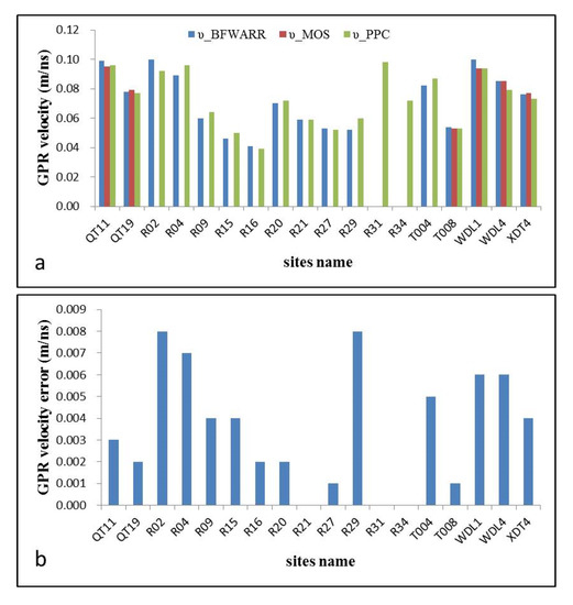
Figure 4.
(a) Velocity comparison acquired by three different GPR detecting methods, blue bar (υ_BFWARR); velocity from wide-angle reflection and refraction methods, red bar (υ_MOS); velocity from multi-offset soundings, green bar (υ_PPC); velocity from pit profile calibration. (b) Absolute error between υ_PPC, υ_BFWARR, and υ_MOS.
3. Results
3.1. Parameters Estimation for Complex Refractive Index Model
In the original Complex Refractive Index Model, the parameters of the dielectric constant should be complex permittivity, which include a real part and an imaginary part. Soil layer (except for saline soil and clay) is generally considered as low-loss media, of which the imaginary part is close to 0 at MHz frequency. So, in our modelling, soil moisture with the Complex Refractive Index Model, only the real part permittivity was applied. This method was also used by many previous researchers for soil moisture modelling [2,3,11,12,13,14,15]. Rearranging Equation (1), soil water content (θ) can be expressed as
For a specific soil type, soil porosity has limited variation under natural conditions. With a pre-determined value of εw and n, Equation (4) can be simply written as
where a can be calculated with εw, εa = 1 and n, and b is an empirical parameter. The dielectric constant of pure water (εw) decreases with an increase in temperature (T). Jones [17] and Meissner [18], respectively, provided εw–T relationship equations for pure water. Their calculated results were equal to the measured data by Atkins [19] for water temperature ranging from 0 °C to 100 °C and Lane [20] from 0 °C to 40 °C According to the data set measured by Atkins, εw can be perfectly fitted with a unary quadratic polynomial within a temperature variation range from 0 °C to 100 °C (Figure 5a, Equation (6)). For the convenience of considering the influence of salinity on the soil water dielectric constant, a very simple straight linear fitting equation was proposed in our research at a partial temperature range from 0 °C to 40 °C, within which the active-layer soil temperature variation range was completely included under natural conditions (Figure 5b, Equation (7)).

Figure 5.
The pure water dielectric constant with temperature variation; (a) water temperature from 0 °C to 100 °C and the unary quadratic linear fitting result; (b) water temperature from 0 °C to 40 °C and the straight linear fitting result.
In Equation (7), α and β are the slope rate and intercept under different soil water salinity; for pure water, α ≈ −0.37 and β ≈ 87.8.
Unlike pure water, a certain amount of salt is dissolved within soil water, even for non-saline soil. Within the temperature range from 0 °C to 40 °C, the dielectric relaxation of aqueous NaCl solutions under different concentrations (0.0, 0.5, 1.0, 1.5, 2.0, 2.5, 3.0 mol/L) is shown in Figure 6 with experiment data from Lane [20].

Figure 6.
Dielectric constant variation with temperature under different concentrations of NaCl solutions (original data from Lane [20]).
The relationships between parameters of α, β in Equation (7) and soil water salinities (S, represented by NaCl concentration in mol/L) was established as follow (Equations (8) and (9)) and shown in Figure 7. Combining Equations (7)–(9), our calculated NaCl solution dielectric constant are almost the same as the laboratory tested result by Lane, with a maximum absolute error of 1.

Figure 7.
(a) Relationship between α and salinity of the NaCl solutions; (b) relationship between β and salinity of the NaCl solution.
The variation range of soil water salinity and temperature within the active layer of the Qinghai–Tibet plateau were analyzed with 11 active-layer monitoring sites along the Qinghai–Tibet highway. Soil water salinity (expressed in terms of NaCl burden) was acquired with a Stevens Hydra Probe (www.stevenswater.com) sensor and soil temperature was acquired with a Model 109 Temperature Probe (www.campbellsci.com/109). The arithmetic mean of all monitoring soil layers’ temperature and soil water salinity from September to October within the active layer was used in our analyzation. Active layer monitoring site name (SN), average soil water salinity (S_mol/L_NaCl), average soil temperature (T/°C), monitoring depth (Depth/cm), layer number of monitoring (LNM), data year (Year) and the calculated soil water dielectric constant (εw) are provided in Table 2. The calculated soil water dielectric constant varied from 85 to 87, and the average was 86. The highest soil water salinity is 0.073 mol/L at site Ch06, which is located at the pass of the Kunlun Mountain. The highest average active-layer temperature is 3.71 °C at site Ch05, which is located at the southern permafrost distribution boundary, named Liangdaohe along the Qinghai–Tibet highway. Site Ch05 is seasonal frozen ground, so it is reasonable to believe that in the plateau permafrost regions, the soil-water temperature within the active layer cannot exceed 3.71 °C. Setting S = 0.073 mol/L and T = 3.71 °C as the upper limit of the soil water condition, S = 0 mol/L(pure water) and T = 0 °C as the lower limit, the average soil water dielectric constant within the active layer correspondingly varies from minimum 84 to maximum 88; its average and median value is also 86. So, in the CRIM of Equation (4), the soil water dielectric constant can be generally determined as a constant value, εw = 86.
Table 2.
The salinity and temperature variation range of active-layer soil water at the Qinghai–Tibet plateau and the calculated water dielectric constant (εw) using Equation (7).
Parameter a in Equation (5) can be acquired through two methods: one is that calculated by εw with a different n value from −1 to 1. The calculated value of a with εw= 86, 84 and 88 (a_εw = 86, a_εw = 84, and a_εw = 88, respectively, in Table 3) were provided in Table 3; the other method is linear fitting through the –θ relationship with a different n number from −1 to 1; here we mark it as a’ in Table 3. The R-squared number (R2) of the –θ linear fitting was also provided. The absolute differences calculated for a with εw between 84 and 88 can be considered as the theoretical maximum absolute error (Error_a); and the absolute differences between a’ and the calculated a (a_εw = 86) with εw = 86 can be considered as the random absolute error (Error_a’), arisen from the error of ε calculated with the GPR velocity at different detecting sites. Comparing Error_a’ and Error_a in Table 3, we found that the parameter n can never be a negative number because of Error_a’ ≫ Error_a. From n = 0.23 to 0.30, Error_a’ is equal to or less than Error_a. We believe that the value of n ranging from 0.23 to 0.3 was acceptable for our experimental data; and we chose n = 0.26, correspondingly a = a’ = 0.458 for the CRIM. What needs to be pointed out is that although Error_a’ is equal to Error_a when n = 0.9 or 1, it should be abandoned because of its lower R-squared number.
Table 3.
Comparison table for determination of parameters a and n in Equation (5).
The parameter b can be acquired through inverse computation of Equation (5) with the measured active-layer soil water content (θ_measured in Table 1), the average b = −0.664. Finally, the CRIM of Equation (5) can be determined as
The calculated active-layer soil water content by our determined CRIM is shown in Figure 8. The average error of the CRIM-calculated result is 0.03 m3/m3 and the maximum error 0.06 m3/m3 for the calculated volumetric soil water content.

Figure 8.
Comparison of CRIM against with measured soil moisture.
3.2. Error Analysis
The main purpose of this paper is to establish a method of utilizing GPR velocity to acquire active-layer soil water content. Velocity error is inevitable during the interpretation of GPR profile data. The interpretation of our field GPR profile revealed that about 0.008 m/ns maximum absolute error existed. In this section, the calculated soil water content error of our determined CRIM (Equation (10)) with a corresponding GPR velocity error of ±0.002 m/ns, ±0.004 m/ns, ±0.006 m/ns, ±0.008 m/ns, and ±0.01 m/ns was analyzed. In addition, a direct linear fitting equation from the relationship between GPR velocity and soil water content was recommended for a large velocity-error GPR profile.
Based on our field GPR detection experience, we assume that the GPR velocity varies from 0.034 m/ns to 0.13 m/ns, which was considered the real GPR velocity. Then, its corresponding dielectric constant and soil moisture (θ) can be calculated with Equations (3) and (10), respectively. If there is a ±0.002 m/ns GPR velocity error, it was added to or subtracted from the assumed real GRP velocity and we get a new velocity, which can be considered as the interpreted GPR velocity. Then another corresponding dielectric constant and θ can be calculated still with Equations (3) and (10), respectively. Finally, the absolute value of the above two calculated θ’s was considered as the calculated θ error caused by the GPR velocity interpreted error. Negative velocity deviation has larger calculated θ errors than the same positive velocity deviation, so we chose negative velocity errors of −0.002 m/ns, −0.004 m/ns, −0.006 m/ns, −0.008 m/ns, and −0.01 m/ns to analyze their influence on θ error, which are shown in Figure 9.

Figure 9.
Calculated θ error with variation in GPR velocity (black line: calculated θ error with CRIM, red line: calculated θ error with direct GPR velocity fitting equation).
From our field GPR detection experience, the lowest GPR velocity within the active layer is 0.034 m/ns, which occurred at a very high organic and water content soil layer, and the highest velocity seldom exceeded 0.13 m/ns. So, the error analysis was discussed within this GPR velocity variation range. From Figure 9 we found that under different GPR velocity interpretation error scenarios, the calculated θ error of CRIM obviously decreases with the increasing of GPR velocity. With a GPR velocity error of less than ±0.004 m/ns, the calculated θ error with CRIM is within 0.08 m3/m3. If we set 0.1 m3/m3 soil water content as the maximum acceptable θ error, the CRIM is unsuitable when the interpreted GPR velocity error is larger than ±0.004 m/ns and GPR velocity is lower than 0.038 m/ns. For example, with a GPR velocity error of −0.006 m/ns, the calculated θ error increased from 0.098 to 0.115 at a GPR velocity range from 0.044 m/ns to 0.034 m/ns. To solve this problem, a direct linear fitting equation between GPR velocity and soil water content was recommended. The scatter plot between GPR velocity and soil water content is shown in Figure 10. This linear fitting equation could be written as
where θ is the soil water content (m3/m3) and υ is the GPR velocity (m/ns). Here we named this soil water moisture calculation as the υ-fitting equation. For our research data, its calculated θ error is similar to CRIM, with an average calculated absolute error of 0.03 m3/m3 and maximum absolute error of 0.06 m3/m3. The advantage of this equation is that its calculated θ error has the same order of magnitude as the υ error, which can be expressed as
where ∆θ is the calculated θ error and ∆υ is the interpreted GPR velocity error. The θ errors calculated by the υ-fitting equation under different GPR velocity interpreted error scenarios are also shown in Figure 9. Unlike CRIM, the calculated θ error with the υ-fitting equation is a constant value. Take a GPR velocity error of ±0.01 m/ns, for example, its calculated θ error is within 0.08 m3/m3. Dividing by a GPR velocity of 0.07 m/ns, the calculated θ error with the υ-fitting equation is obviously lower than with CRIM when the GPR velocity is lower than 0.07 m/ns. When the GPR velocity is higher than 0.07 m/ns, the calculated θ error with the υ-fitting equation is obviously higher than with CRIM. So, when the GPR velocity interpretation error is larger than ±0.004 m/ns and the velocity is lower than 0.07 m/ns, this υ-fitting equation is recommended to avoid large soil water content calculation error with CRIM.

Figure 10.
Scatter diagram of the relationship between GPR velocity and active-layer soil moisture.
4. Discussion: Representativeness and Applicability
In order to evaluate the applicability of the CRIM and υ-fitting equation to the Qinghai–Tibet plateau permafrost regions, the representativeness of our field investigation sites have to be analyzed. The difference in soil texture, which can be indirectly reflected by soil bulk density and organic content, is the main reason for the calibration of petrophysical relationship between soil permittivity and soil water content. So, the influences of soil organic content and soil density on active-layer soil moisture calculation and the representativeness of our GPR sites were analyzed in this section.
4.1. Influence of Soil Organic Content
Compared to mineral soil, organic soils typically have lower bulk densities (or higher porosities) and larger specific surface areas than mineral soil. Laboratory tests by Zhaoqiang [21] pointed out that, for dried soil, the dielectric constant appeared to decrease with the increase of soil organic content. His experiment also concluded that the dried soil dielectric constant decreases with the decreasing of soil bulk density. So, with the same dielectric constant value, organic soil will have more water content than mineral soil.
Specifically for organic soil, many researchers had developed calibration curves and their results were summarized and compared by Lange [22] and Bircher [23]. Among these organic soil calibration curves, we chose these that are close to our data, which were recommended by Roth [8], to analyze the influence of soil organic content on the soil water content calculation. Figure 11 showed calibration curves of organic content at 10.5% and 54.8% (θ_Roth_organic_10.5%, θ_Roth_organic_54.8%), and the bulk composited curve of mineral soils with a sand content range from 2% to 88% (θ_Roth_mineral_bulk). The comparison of the three Roth’s calibration curves revealed that under the same dielectric constant, organic soil generally has higher water content than mineral soil under the same soil dielectric constant conditions. The influence of organic content on soil water content calculation can also be found with our data. Depth-weighted average organic contents within the active layer on our research regions varied from 0.3% to 17.5% (Table 1). There are two pairs of data points in which we can find the influence of organic content. R34 and R20 have the same dielectric constant of 17. For the former, which had an organic content of 4.0%, the measured soil water content was 0.04 m3/m3 higher than the latter, which had an organic content of 1.7%. R29 and R21 appeared to have similar dielectric constants of 25 and 26, respectively. For the former, which had an organic content of 9.9%, the measured soil water content was 0.05 m3/m3 higher than the latter, which had an organic content of 3.9%. Although there were water content differences arising from organic content variation, the magnitude of deviation and the excellent performance of our acquired CRIM reminded us that the influence of organic content can be neglected at least at an organic content level below 17.5% for the active-layer soil moisture calculation.
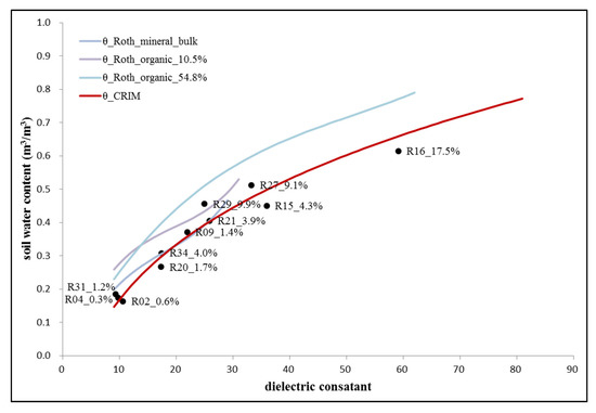
Figure 11.
Comparison of organic and mineral calibration curves against our measured soil water content of different organic contents.
In the Qinghai–Tibet plateau permafrost region, active-layer thicknesses are nearly 100 cm all over. Take the Qinghai–Tibet highway, for example, which is across the north and south borders of the permafrost distribution on the plateau, and where active-layer thicknesses varied from 100 cm to 350 cm [24]. From 2009 to 2013, large-scale investigations of permafrost and active layer thickness distribution on the Qinghai–Tibet plateau were carried out from July to October. Total numbers of more than 200 pits were dug. We choose 128 pits with depths exceeding 100 cm to statistically analyze organic content distribution on the plateau. Our analyzed result presented that on the Qinghai–Tibet plateau, depth-weighted average organic contents within the active layer were below 12% (Figure 12). This organic content level is lower than the highest organic content of our analyzed GPR site R16 (SOM, 17.5%), which is not included in Figure 12 because its pit depth was less than 1 m (0.6 m). Considering the general organic matter content level within the active layer on the Qinghai–Tibet plateau, it is reasonable to speculate that our selected data samples, which were used for the establishment of CRIM, can fully represent the active layer organic distribution condition on the plateau permafrost regions.

Figure 12.
Active-layer soil organic content variation on the Qinghai–Tibet plateau.
4.2. Influence of Soil Bulk Density
Average active-layer soil bulk densities of our GPR detecting sites varied from 0.6 g/cm3 to 1.8 g/cm3 (Table 1). Similar to the analysis of organic influence, 125 pits with depths exceeding 100 cm were chosen to statistically analyze bulk density distribution on the plateau. Our statistical analysis shows that average active-layer soil bulk densities varied from 0.8 g/cm3 to 2.1 g/cm3. Most of the pits’ average densities were within 1.8 g/cm3 (about 91% of the total analyzed 125 pits), which can be represented by our GPR detecting sites (Figure 13a). In addition, the influence of soil density on the relationship between the dielectric constant and soil moisture within the active layer were analyzed with Figure 13b. On the whole, with the increase in soil water content or the dielectric constant, its bulk density decreased. This is reasonable because for a higher water content region, the soil organic content within the active layer is often higher, which results in lower soil bulk density. Unlike organic content, the influence of soil bulk density variation on the relationship between the soil dielectric content and soil moisture is not obvious. For example, the density of five GPR detecting sites is 1.5 g/cm3 (red points in Figure 13b). Their dielectric constant variation can be found mainly influenced by soil water content, and these data points randomly scattered within the whole data series. So, it is reasonable to conclude that the influence of soil bulk density on the establishment of active-layer soil moisture calibration curves can also be neglected for the Qinghai–Tibet plateau permafrost regions.

Figure 13.
(a) Statistical histogram of the active-layer soil density variation on the Qinghai–Tibet plateau. (b) Scatter diagram of the relationship between the soil dielectric constant and moisture under different soil bulk densities.
5. Discussion
Although only 18 field-investigated active layer data were available in our research, their soil water content varies at a very large scale, ranging from 0.124 cm3/cm3 to 0.614 cm3/cm3, and very different vegetation type, including bare land, grass land, meadow, and wet meadow, were covered by our data samples. In our opinion, these data samples, by and large, can represent the active-layer soil water content variation range of the Qinghai–Tibet plateau permafrost regions.
Many published papers concluded that organic soil has a very different soil water content calibration curve from mineral soil [23]. Although the influence of organic content can be recognized with our data, i.e., higher organic content soil has higher soil water content under the same soil dielectric condition, the small deviation of our measured soil water content from the CRIM calibration curve demonstrated that the active-layer soil profile, as a whole soil profile, can be considered as the single soil type with an organic content level at least lower than 17.5%.
Field investigation on the Qinghai–Tibet plateau permafrost regions revealed that the average active-layer soil profile densities varied from 0.8 g/cm3 to 2.1 g/cm3. The average active-layer soil profile densities at our GPR detecting sites varied from 0.6 g/cm3 to 1.8 g/cm3, which cover most of the density variation range on the Qinghai–Tibet plateau. Soil density can be indirectly used to represents soil texture and soil grain size level, which in turn directly influence the two parameters of soil matrix dielectric constant and porosity within the Complex Refractive Index Model. The soil with high bulk density means it has low porosity, and vice versa. The dielectric constant of the soil matrix often varies from 3 to 7 [25], which is larger than air’s dielectric constant of 1. So, high bulk density soils have high dielectric values under dry conditions. The water’s dielectric constant is one magnitude of order larger than soil particles and air, and the soil bulk dielectric is mainly influenced by the ratio of soil water content and the influence of soil texture, and grain size level can be neglected for soil moisture estimation. The laboratory experiment by Yuanshi [26] revealed that each 0.1 g/cm3 increase in soil bulk density will result in a −0.004 cm3/cm3 measurement error in soil water content with a TDR sensor, which means that a 1 g/cm3 soil density difference only has a 0.04 cm3/cm3 soil water calculation error, which is smaller than or equivalent to many soil moisture calibration curves’ calculated errors. So, in our opinion, the influence of soil density on soil water measurement with GPR can be neglected, especially for large-scale investigation.
Through the influence analysis of soil organic content and soil density on soil water calculation with our GPR detection soil samples, we found that organic content has a more apparent impact than soil density. Our GPR detection soil samples were all distributed on the eastern part of the Qinghai–Tibet plateau, which is high soil organic distribution regions. It is well known that soil organic content is often high in good vegetation distribution regions. From a previous study, alpine meadows mainly distribute on the eastern part, and alpine steppe and desert mainly distribute on the western part of the Qinghai–Tibet plateau [27]. From the previous Figure 12, we also can find that active-layer average organic content from the eastern part (serial number from 1 to 70) is obviously higher than from the western part (serial number from 71 to 128). Our GPR detection soil samples all came from eastern part (Figure 14) and their organic content varied from 0.3% to 17.5%. We believe that this variation range can also include the highest organic content level from Qinghai–Tibet west regions and the CRIM and υ-fitting equations can also be applied in this region. More generally, because soil organic content is the main influence of the difference of soil moisture calibration equations, we believe that this CRIM equation can also be applied in other research regions where the soil organic content is lower than 17.5%.

Figure 14.
Spatial distribution of our GPR detection soil sample sites and all the active layer pits for organic content and soil bulk density analysis.
By comparing our derived soil moisture calibration equations, CRIM andυ-fitting, with other previous equations, we found that the Topp equation is the closest to the calibration curves (Figure 15a). At the soil dielectric constant (ε) variation range from 5 to 26 or from 65 to 70, of which the corresponding converted GPR velocity is from 0.134 m/ns to 0.059 m/ns or from 0.037 m/ns to 0.036 m/ns, the calculated soil moisture with CRIM is slightly lower than with Topp, but their absolute deviation are within 0.05 m3/m3 (Figure 15b). Because the dielectric constant of the saturated low organic soil layer is hard to get past 70 under natural conditions, so the CRIM equation and Topp equation can be considered as equivalent equations if we can accurately measure the soil dielectric constant. But when the Topp equation is applied for soil moisture calculation with GPR velocity, its calculation error sharply increases when GPR velocity is lower than 0.05 m/ns, and its maximum error may exceed 0.1 m3/m3 even if the GPR velocity interpretation error is within ±0.002 m/ns. For the υ-fitting equation, its absolute deviation from the Topp equation is within 0.05 m3/m3 at the dielectric constant variation range from 19 to 56, of which the corresponding converted GPR velocity is from 0.069 m/ns to 0.040 m/ns (Figure 15b). The Topp equation was derived from laboratory tests with different representative mineral soil samples and was well accepted by other researchers on different regions, so we believe that our derived CRIM and υ-fitting equation can also be applied in other low organic content distribution regions and they are more suitable for soil moisture estimation with GPR detection.
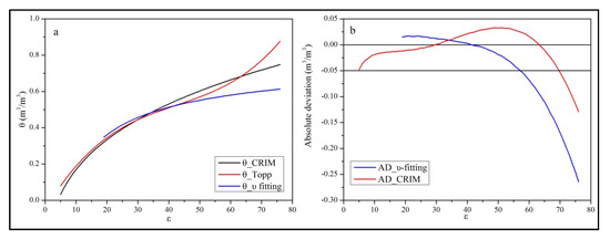
Figure 15.
Comparisons between CRIM,υ-fitting equations and the Topp equation (a) and their absolute deviation (b).
6. Conclusions
In this research paper, we used 18 active layer GPR detecting pits that were distributed in different areas in the Qinghai–Tibet plateau permafrost region to construct active-layer soil moisture measure methods with GPR signal travel speed. Based on the soil physics model, the active-layer soil water dielectric constant (εw = 86) and the experienced exponent parameter (n = 0.26) were theoretically deduced. Finally, we acquired the semi-empirical physical model, CRIM, that was suitable for active-layer soil moisture calculation with a dielectric constant in the Qinghai–Tibet plateau permafrost regions. When the GPR velocity interpretation error is within ±0.002 m/ns, the calculated soil moisture absolute error will not exceed 0.05 m3/m3. When the GPR velocity interpretation error is within ±0.004 m/ns, the calculated soil moisture absolute error will not exceed 0.08 m3/m3. In order to avoid the calculated soil water content error aroused from GPR velocity interpretation error at sites where GPR velocity is lower than 0.07 m/ns, a υ-fitting equation between GPR velocity and soil water content was acquired and proposed based on our field-investigated data. Within the GPR velocity variation range of below 0.07 m/ns, the calculated θ error by υ-fitting equation is obviously lower than CRIM and will not exceed 0.08 m3/m3 under an interpreted GPR velocity maximum error of 0.01 m/ns. So, when GPR velocity interpretation error is larger than ±0.004 m/ns, a piecewise formula calculation method, combined with a υ-fitting equation when the GPR velocity is lower than 0.07 m/ns and a CRIM equation when the GPR velocity is larger than 0.07 m/ns, was recommended for the active layer moisture estimation with GPR detection. Through the analysis of influences of soil organic content and soil density on active-layer soil moisture calculation, and of the representativeness of our investigated sites, our conclusion is that the semi-empirical CRIM and υ-fitting equation is not only suitable for our investigated sites, but can also be applied in the Qinghai–Tibet plateau permafrost regions.
Author Contributions
In preparing this research paper, E.D., L.Z. and R.L. were responsible for the conceptualization and writing—review and editing; writing—original draft preparation was finished by E.D.; the investigation of active layer pits were conducted by Z.W., X.W., G.H., Y.Z. and G.L.; GPR detection was conducted by E.D., D.Z. and Z.S.; E.D. finished the GPR data post-processing. All authors have read and agreed to the published version of the manuscript.
Funding
This research was funded by National Natural Science Foundation of China (grant numbers: 41301066, 41931180, 41701073 and 41701077), the State Key Laboratory of Cryospheric Science (SKLCS-ZZ-2018) and the Excellent Youth Scholars of Northwest Institute of Eco-Environment and Resources, CAS.
Acknowledgments
We really appreciate the modification and useful amending advice for this manuscript from Liu Lin and Ph. D student Yan Liu in the Chinese University of Hong Kong.
Conflicts of Interest
The authors declare no conflicts of interest.
References
- Kirkham, M.B. Time Domain Reflectometry. In Principles of Soil and Plant Water Relations, 2nd ed.; Kirkham, M.B., Ed.; Academic Press: Boston, MA, USA, 2014; pp. 103–122. [Google Scholar] [CrossRef]
- Huisman, J.A.; Hubbard, S.S.; Redman, J.D.; Annan, A.P. Measuring Soil Water Content with Ground Penetrating Radar: A Review. Vadose Zone J. 2003, 2, 476–491. [Google Scholar] [CrossRef]
- Parsekian, A.D.; Slater, L.; Gimenez, D. Application of ground-penetrating radar to measure near-saturation soil water content in peat soils. Water Resour. Res. 2012, 48, 02533. [Google Scholar] [CrossRef]
- Chen, A.; Parsekian, A.D.; Schaefer, K.; Jafarov, E.; Panda, S.; Liu, L.; Zhang, T.; Zebker, H. Ground-penetrating radar-derived measurements of active-layer thickness on the landscape scale with sparse calibration at Toolik and Happy Valley, Alaska. Geophysics 2016, 81, H9–H19. [Google Scholar] [CrossRef]
- Liu, L.; Schaefer, K.; Gusmeroli, A.; Grosse, G.; Jones, B.M.; Zhang, T.; Parsekian, A.D.; Zebker, H.A. Seasonal thaw settlement at drained thermokarst lake basins, Arctic Alaska. Cryosphere 2014, 8, 815–826. [Google Scholar] [CrossRef]
- Koyama, C.N.; Liu, H.; Takahashi, K.; Shimada, M.; Watanabe, M.; Khuut, T.; Sato, M. In-Situ Measurement of Soil Permittivity at Various Depths for the Calibration and Validation of Low-Frequency SAR Soil Moisture Models by Using GPR. Remote. Sens. 2017, 9, 580. [Google Scholar] [CrossRef]
- Topp, G.C.; Davis, J.L.; Annan, A.P. Electromagnetic determination of soil water content: Measurements in coaxial transmission lines. Water Resour. Res. 1980, 16, 574–582. [Google Scholar] [CrossRef]
- Roth, C.H.; Malicki, M.A.; Plagge, R. Empirical evaluation of the relationship between soil dielectric constant and volumetric water content as the basis for calibrating soil moisture measurements by TDR. J. Soil Sci. 1992, 43, 1–13. [Google Scholar] [CrossRef]
- Zamolodchikov, D.; Karelin, D.V.; Ivaschenko, A.I.; Oechel, W.C.; Hastings, S.J. CO2 flux measurements in Russian Far East tundra using eddy covariance and closed chamber techniques. Tellus B Chem. Phys. Meteorol. 2003, 55, 879–892. [Google Scholar] [CrossRef]
- Engstrom, R.; Höpe, A.; Kwon, H.; Stow, D.; Zamolodchikov, D. Spatial distribution of near surface soil moisture and its relationship to microtopography in the Alaskan Arctic coastal plain. Hydrol. Res. 2005, 36, 219–234. [Google Scholar] [CrossRef]
- Birchak, J.; Gardner, C.; Hipp, J.; Victor, J. High dielectric constant microwave probes for sensing soil moisture. Proc. IEEE 1974, 62, 93–98. [Google Scholar] [CrossRef]
- Alharthi, A.; Lange, J. Soil water saturation: Dielectric determination. Water Resour. Res. 1987, 23, 591–595. [Google Scholar] [CrossRef]
- Roth, K.; Schulin, R.; Flühler, H.; Attinger, W. Calibration of time domain reflectometry for water content measurement using a composite dielectric approach. Water Resour. Res. 1990, 26, 2267–2273. [Google Scholar] [CrossRef]
- Comas, X.; Slater, L.; Reeve, A. Spatial variability in biogenic gas accumulations in peat soils is revealed by ground penetrating radar (GPR). Geophys. Res. Lett. 2005, 32, 08401. [Google Scholar] [CrossRef]
- Dobson, M.; Ulaby, F.; Hallikainen, M.; El-Rayes, M. Microwave Dielectric Behavior of Wet Soil-Part II: Dielectric Mixing Models. IEEE Trans. Geosci. Remote. Sens. 1985, GE-23(1), 35–46. [Google Scholar] [CrossRef]
- Diamanti, N.; Elliott, E.J.; Jackson, S.R.; Annan, A.P. The WARR machine: system design, implementation and data. J. Environ. Eng. Geoph. 2018, 23, 469–487. [Google Scholar] [CrossRef]
- Jones, S.B.; Blonquist, J.M.; Robinson, D.A.; Rasmussen, V.P.; Or, D. Standardizing Characterization of Electromagnetic Water Content Sensors: Part 1. Methodology. Vadose Zone J. 2005, 4, 1048–1058. [Google Scholar] [CrossRef]
- Meissner, T.; Wentz, F. The complex dielectric constant of pure and sea water from microwave satellite observations. IEEE Trans. Geosci. Remote. Sens. 2004, 42, 1836–1849. [Google Scholar] [CrossRef]
- Atkins, R.T.; Pangburn, T.; Bates, R.E.; Brockett, B.E. Soil moisture determinations using capacitance probe methodology. Special report 98-2, US Army Corps of Engineers, Cold Regions Research & Engineering Laboratory. 1998. Available online: https://apps.dtic.mil/dtic/tr/fulltext/u2/a337497.pdf (accessed on 1 July 2019).
- Lane, J.A.; Saxton, J.A. Dielectric dispersion in pure polar liquids at very high radar frequencies, III, The effect of electrolytes in solution. Proc. R. Soc. Lond. 1952, 214, 531–545. [Google Scholar] [CrossRef]
- Zhaoqiang, J. Dielectric permittivity and its relationship with water content for several soils in China. Master’s Thesis, China Agricultural University, Beijing, China, 15 June 2005. [Google Scholar]
- Lange, S.F.; E Allaire, S.; Juneau, V. Water content as a function of apparent dielectric permittivity in a Fibric Limnic Humisol. Can. J. Soil Sci. 2008, 88, 79–84. [Google Scholar] [CrossRef]
- Bircher, S.; Andreasen, M.; Vuollet, J.; Vehviläinen, J.; Rautiainen, K.; Jonard, F.; Weihermüller, L.; Zakharova, E.; Wigneron, J.-P.; Kerr, Y.H. Soil moisture sensor calibration for organic soil surface layers. Geosci. Instrum. Methods Data Syst. 2016, 5, 109–125. [Google Scholar] [CrossRef]
- Li, R.; Zhao, L.; Ding, Y.; Wu, T.; Xiao, Y.; Du, E.; Liu, G.; Qiao, Y. Temporal and spatial variations of the active layer along the Qinghai-Tibet Highway in a permafrost region. Chin. Sci. Bull. 2012, 57, 4609–4616. [Google Scholar] [CrossRef]
- Cihlar, J.; Ulaby, F.T. Dielectric properties of soils as a function of moisture content. CRES Technical report-177-47, The University of Kansas Space Technology Center Raymond Nichols Hall; 1974. Available online: https://ntrs.nasa.gov/archive/nasa/casi.ntrs.nasa.gov/19750018483.pdf (accessed on 30 July 2019).
- Yuanshi, G.; Qiaohong, C.; Zongjia, S. The effects of soil bulk density, clay content and temperature on soil water content measurement using time-domain reflectometry. Hydrol. Process. 2003, 17, 3601–3614. [Google Scholar] [CrossRef]
- Wang, Z.-W.; Zhao, L.; Wu, X.-D.; Yue, G.-Y.; Zou, D.-F.; Nan, Z.-T.; Liu, G.-Y.; Pang, Q.-Q.; Fang, H.-B.; Shi, J.-Z.; et al. Mapping the vegetation distribution of the permafrost zone on the Qinghai-Tibet Plateau. J. Mt. Sci. 2016, 13, 1035–1046. [Google Scholar] [CrossRef]
© 2020 by the authors. Licensee MDPI, Basel, Switzerland. This article is an open access article distributed under the terms and conditions of the Creative Commons Attribution (CC BY) license (http://creativecommons.org/licenses/by/4.0/).