Abstract
The current full-waveform data at a single wavelength can mainly retrieve the geometric attributes of targets along the light path by detecting waveform components, resulting in the lack of spectral or color attribute information. This kind of device relies on a digital camera for acquiring the color information, however, which is inevitably limited by the lighting conditions and geometric registration errors. With the development of multispectral light detection and ranging (LiDAR) or even hyperspectral LiDAR that often utilize a supercontinuum laser source covering the whole visible light band, including red, green and blue bands, the simultaneous acquisition of color and spatial information becomes possible and makes passive imaging data no longer necessary. In this study, we propose a color restoration method for a full-waveform multispectral LiDAR (FWMSL) system. Additionally, we develop a multispectral lognormal function to fit the tailing echoes measured by FWMSL further accurately. Experimental data from our FWMSL system are used to evaluate the performance of the proposed method. The relative standard deviation, correlation coefficient (R2) and color difference () metrics suggest that the color restoration for the full-waveform multispectral data is feasible.
1. Introduction
Light detection and ranging (LiDAR) system has been known as one of the most effective survey tools to characterize vegetation structure for the past decades because of its excellent ranging accuracy and canopy penetration capability [1,2]. The emerging full-waveform LiDAR (FWL) system can record the entire backscatter waveform echo, providing an opportunity for researchers to explore the waveform data further, thereby obtaining the physical properties of the target with increased accuracy and reliability [2,3]. The shape features (e.g., central location, pulse width and amplitude) extracted from waveform data [1,4] are greatly helpful in various applications, such as land cover classification [5], building extraction [6,7], canopy height retrieval [8] and biomass estimation [9].
Reflective and texture features of the target surface are also required to meet the application needs as mentioned above. However, the current full-waveform data at a single wavelength can mainly retrieve the geometric attributes of targets along the light path by detecting waveform components, resulting in the lack of spectral or color attribute information. The existing methods mainly collect the texture and spectral data by the fusion of passive image data such as multispectral image [10]. Since the passive imaging sensors rely on solar illumination, certain inevitable errors are caused by geometric registration between the active and passive datasets. Although many studies have focused on solving the geometric registration problems and achieved high registration accuracy [11,12,13], considerable time and labor are still needed to achieve a satisfactory registration effect.
In recent years, the development of multispectral LiDAR (MSL) or even hyperspectral LiDAR (HSL) systems [14,15,16,17,18] have effectively increased the receiving channels of full waveform data for interest wavelengths. These new MSL/HSL systems often utilize a supercontinuum laser source which produces broadband light almost covering the whole visible light band, including red (R), green (G) and blue (B) bands [19]. Thereby, the simultaneous acquisition of texture and spatial information becomes possible and makes passive imaging data no longer necessary. In terms of obtaining color with LiDAR data directly, Bretagne et al. [20] attempted to interpret intensity as a green level in RGB or sRGB color spaces under standard illuminant of International Commission on Illumination (CIE) by using a commercial single wavelength LiDAR device at 532 nm. Although the statue faces appear clear and homogeneous with the G level, the color information is still incomplete to visualize the real scene. Conversely, since the multispectral full-waveform data could cover the whole RGB bands, it has great potential in restoring the complete color information directly without fusion of any passive images.
For the multispectral full-waveform data, it reflects the interaction between all targets along the light path at multiple receiving channels, mixed with a variety of texture and spatial information in the waveforms. To date, such types of data have not been tested to extract color information. Consequently, the overall goal of this paper is to develop a color restoration method for the full-waveform data at RGB bands in order to extract the color information directly and efficiently, thus avoiding the adverse effects of registration and solar illumination. The objectives of this study are to: (1) propose a theoretical model for color restoration for the multispectral full-waveform data at RGB bands; (2) perform the color restoration method with measured multispectral waveform data to verify the feasibility and efficiency of the new method.
2. FWMSL System
In the past few years, we have been committed to the development of MSL. We used four solid-state lasers at 556, 670, 700 and 780 nm with full-waveform recording of the receiving channels for monitoring the growth and nutritional status of vegetation. The previous MSL was effective in capturing abundant biochemical information of vegetation [15] and had increased waveform decomposition accuracy [14]. Given its significant improvement in vegetation detection, we found that directly synthesizing the true color of targets based on these selected laser bands remains difficult due to the lack of a B band laser source, which results in low visualization and limits the capability to render the true surface color of the target. Although the B band is insensitive to vegetation, it is necessary for restoring the B value in the RGB color space. Therefore, we further updated our MSL with a supercontinuum laser (NKT Photonics, SuperK) source, which covers a wide range of wavelengths, including almost the entire visible band (400–700 nm), instead of the synthesis of multiple laser sources. The laser has a repetition rate of 20 kHz with average power of 100 mW.
We have analyzed the results of true color synthesis through different wavelength combinations for an HSL system and found that the most suitable RGB wavelength combination is 466, 546 and 626 nm [21]. Meanwhile, on the basis of the principle of supercontinuum laser, the broad-spectrum laser is always pumped with the seed laser at a fundamental frequency of 1064 nm, which is far from the visible band, resulting in a relatively low output energy in the short band but the energy increases sharply from around 450 nm (Figure 1a). Therefore, we have selected three wide bands near the corresponding wavelengths, especially for the blue band which is relatively wide, in order to increase the energy of the RGB channels to obtain a higher signal-to-noise ratio (SNR). Considering the spectral energy distribution of the supercontinuum laser source and CIE 1931 color space chromaticity (Figure 1b), the RGB bands, namely, 434.5–474.5, 517–537 and 612–644 nm, in the visible spectral portion were selected for the receiving channels of color information. In addition, the photo multiplier tube (PMT) selected as the detector should be more suitable for detecting laser echoes in visible bands than the avalanche photodiode especially in the relatively low-energy B band since PMT has higher quantum efficiency and gain. Moreover, both the transmitted pulse and receiving echo at RGB bands are full-waveform recorded so that the receiving echoes can be calibrated with the transmitted pulses to eliminate errors caused by laser output energy instability. The waveforms of the three receiving channels were digitized in a 12-bit analog to digital converter (SP Devices, ADQ412), with a 1.8 GHz sampling rate. The length of each active signal is set to 20 samples based on the laser pulse width of 2 ns and sampling rate, thus greatly reducing the amount of data.
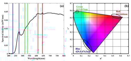
Figure 1.
(a) Output spectral power distribution curve of the supercontinuum laser source. (b) CIE 1931 color space chromaticity diagram. The outer curved boundary is the spectral (or monochromatic) locus and the selected RGB bands are presented on the boundary.
3. Methods and Materials
3.1. Color Restoration Method For FWMSL
To our knowledge, most existing color restoration methods are for fusing passive image data such as multispectral images with the three-dimensional point clouds. In this case, the camera is equipped with a color filter array, only one of the RGB values is recorded at each pixel and the other two values are interpolated by adjacent pixels [22,23]. For the FWMSL system, the entire backscattered echo waveform from RGB channels are recorded simultaneously, which can be used to retrieve the true RGB values of each measured point without interpolation. Therefore, the process of retrieving color information from the echo waveform of each pulse becomes particularly important.
The flowchart of color restoration for the multispectral full-waveform data is displayed in Figure 2. First, waveform fitting is performed to obtain waveform parameters that can be used to express the backscattering intensity of targets. Next, the RGB values are retrieved from corresponding backscattering intensity since the RGB values are proportional to the target reflectivity in the RGB bands [20]. Moreover, the pulses are accumulated to improve the SNR of the echoes, thus helping the accuracy of color restoration further.
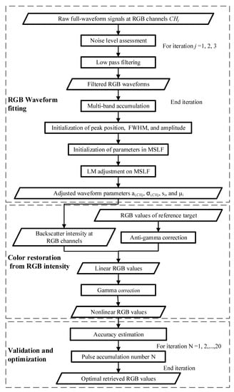
Figure 2.
Flowchart of color restoration, consisting of RGB waveform fitting, color restoration from RGB intensity and validation and optimization.
3.1.1. RGB Waveform Fitting
On the basis of prevailing methods, a full-waveform echo is commonly fitted using several symmetrical Gaussian functions [3,24,25] and each function corresponds to an echo component. However, given that the rise time of the PMT of the FWMSL system is as short as 0.6 ns and the discharge is slow, the return echo components recorded by FWMSL are asymmetrical. The fitting process has low accuracy when the echo components are asymmetrical but fitted by using the symmetrical Gaussian function.
Figure 3 shows the comparison between Gaussian and lognormal functions to fit the raw waveform data detected by PMT. The lognormal function has a short rise time and a tailing, which fits the echo more accurately than Gaussian. In particular, the peak position detected by the Gaussian function is right biased due to the tailing. Therefore, we select the lognormal function [26] to describe the echo components. The lognormal function can be expressed as
where is the fitting model for the ith echo component, is the amplitude of the ith echo component, is the standard deviation of the ith echo component and and are related to the offset of the ith echo component. The correspondence between the parameters in Equation (1) and the physical properties of the target need be further explored. The physical properties of the target, that is, backscatter characteristic, distance and surface roughness, are reflected in the waveform component. The peak value of the waveform component is related to the backscatter characteristic, the peak position of the waveform component reflects the distance and the full width at half maximum (FWHM) of the waveform component is related to the surface roughness. Thus, the parameters in Equation (1) can be used to describe the corresponding physical properties of the target. As the zero-crossing point of the first derivative of the component is the peak point, the peak position can be expressed as Equation (2), determined by and . Additionally, FWHM can be expressed as Equation (3) on the basis of its definition, determined by and .
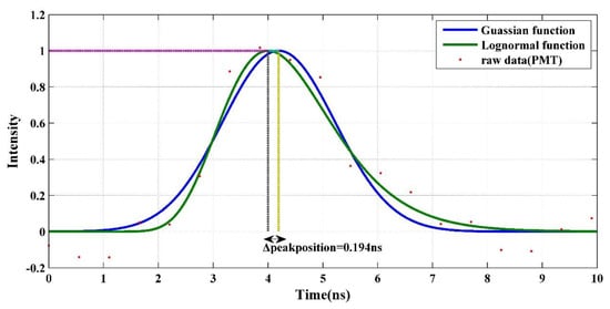
Figure 3.
Comparison between Gaussian (continuous line) and lognormal (dotted line) functions.
Based on the above derivation, the lognormal function not only approximates the asymmetrical echo waveform but also reflects the physical properties of targets. However, this function ignores the correlation between bands, which causes the waveform components of each band to contradict each other in spatial distribution. In theory, each band should exhibit the same location distribution. Therefore, parameters and are independent of the band according to Equation (2). Meanwhile, parameters and are different at each band because of the reflectance of the target, the pulse width of the outgoing pulse and the response of the detector dependent on the band. Accordingly, we develop a multispectral lognormal function (MSLF) expressed as
where denotes the modeled waveform as a function of time (x) at the band of . and are related to the band of corresponding to the ith echo component. and are related to the distance of the ith echo component independent of the band. is the background noise of the signal at the band of .
The MSLF-based RGB waveform fitting process mainly includes three steps, noise level estimation, parameter initialization and parameter optimization.
Noise level estimation. The noise level must be estimated first so that the fitting threshold can be set accordingly. The mean and standard deviation of the background noise are calculated from the head or tail of the signal and denoted as and , respectively. The amplitude of the active signal is generally considered to be higher than three times the standard deviation of the noise [8,24,27,28]. Thus, the noise threshold of the laser echo is denoted as , expressed as . Generally, the fitting process should satisfy three criteria: the FWHM of the component is no less than that of the transmitted pulse , the amplitude of the component is more than three times the standard deviation of the background noise signal and the waveform fitting error (root mean square error [RMSE]) is less than three times the standard deviation of the background noise signal, expressed as Equation (5).
where the subscript CHj corresponds to one of the RGB channels.
Parameter initialization. The active signal is separated from the noise after the noise threshold is determined. The peak and inflection points are parts of the active signal; thus, their intensities are greater than the noise threshold (). The zero-crossing points of the first derivative of the echo are considered to be peak points corresponding to the amplitude and central location of the echo component. The zero-crossing points of the second derivative are inflection points corresponding to the standard deviation of the echo component. However, the derivatives of the laser echo have many spikes due to the existence of noise. The spikes may produce false zero-crossing points. To avoid false peak and inflection points, the waveform signal is smoothed with a low pass filter whose width is set as the width of the transmitted pulse. Then, the peak and inflection points can be searched on the smoothed waveform echo.
The target is likely to show high reflectance in one band while low in another. Since the waveforms at RGB bands should have the same position distribution, we accumulate the three waveforms in order to improve the SNR, thus helping retrieve shape parameters. Initialization using multispectral waveforms shows great potential in providing more complete, accurate parameter estimation. Echo components exist roughly at the position where the peak points (, ) lie, where and represent the location and intensity of the peak point, respectively. The parameters peak position and FWHM are initialized based on the peak points and corresponding inflection points of the multi-band accumulated waveform. The amplitudes at RGB bands are then initialized using the waveform at the corresponding band. After initialization of amplitude, peak position and FWHM, the parameters in MSLF are then calculated according to Equations (2) and (3). The components will be regarded as false and removed if the amplitude is less than the noise threshold or the FWHM is less than that of the transmitted pulse.
Parameter optimization. The Levenberg-Marquardt (LM) optimization is applied to the initially estimated parameters of MSLF to approximate the raw waveform data. The LM iteration after accurate initialization performs more efficient and is less likely to fall into local optimization. During parameter optimization, potential echo components are added to MSLF ordered by energy level calculated as . The components will be regarded as false and removed if the amplitude is less than the noise threshold or the standard deviation is less than that of the transmitted pulse. Parameter optimization ends when all potential echo components are added to the function or when the RMSE is smaller than three times the standard deviation of the background noise signal.
After the parameter optimization, shape parameters at RGB bands that can be used to describe the waveform are available. Then, using these parameters to reasonably express the reflection information of the target becomes important, thus preparing for the next color restoration. The backscatter intensity is traditionally recorded as peak value of the raw waveform, which contains many random errors. However, in this study, the backscatter intensity is represented by the amplitude () and integral area of the fitted waveform (). The performance of these two expressions will be evaluated later.
3.1.2. Color Restoration from RGB Intensity
Color is the sensation created in response to excitation of the human eyes after the combined effect of ambient light and the reflective properties of targets [29]. The reflective properties of targets are related to the backscatter intensity obtained in Section 3.1.1. In comparison with passive imaging in which image quality is strongly dependent on background light source, the FWMSL system obtains the reflective properties of targets without the limitation of background light source. Moreover, various standard light sources are defined by CIE, among which illuminant D65 is commonly used as average daylight. Therefore, we assume that ambient light conditions are consistent with CIE standard illuminant D65. In other words, the color restored in this study is under illuminant D65.
The linear RGB values are proportional to the backscattered intensity from RGB channels. To obtain the RGB values of an unknown target, a reference target whose linear RGB values are known under illuminant D65 is needed. The standard whiteboard is select as the reference target, the linear RGB values of which are (1, 1, 1). Additionally, the corresponding backscattered intensity I can be obtained as mentioned in Section 3.1.1. Then, the linear RGB values RL, GL and BL under illuminant D65 are calculated as
where IR, IG and IB are the backscattered intensity of targets from RGB channels. RL0, GL0 and BL0 are the linear RGB values of the reference target that are known under CIE standard illuminant D65. IR0, IG0 and IB0 are the backscattered intensity of the reference target from RGB channels.
However, the direct display of the linear RGB values will be distorted, as the cathode ray tube (CRT) in the monitor has a power law response to the applied voltage that is proportional to the digital RGB values, as shown in Figure 4a. In other words, the monitor shows a nonlinear transformation of the input RGB values. To eliminate the color distortion caused by the nonlinear response of the CRT, we initially perform gamma correction (Figure 4b) on the linear RGB values. The Gamma coefficient for different display devices is a little different, usually set to 2.2. The nonlinear RGB values are calculated as defined in IEC 61966-2-1 using gamma correction as
where RL, GL and BL are the linear RGB values of targets. represents the gamma factor.
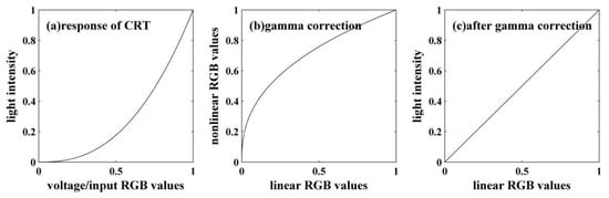
Figure 4.
(a) Cathode ray tube (CRT) in the monitor has a power law response to the applied voltage or input RGB values. (b) Linear RGB values are transformed to nonlinear RGB values with gamma correction. (c) Nonlinear RGB values instead of linear RGB values are input into the CRT and the color displayed is consistent with the original linear RGB values.
After gamma correction, the nonlinear RGB values are input to the display device, thus finally converted into linear light consistent with the original color by the CRT (Figure 4c). Therefore, the retrieved color in this paper is a set of non-linear RGB values, which can be directly applied to the display device and the visual effect is consistent with the real scene.
3.1.3. Validation and Optimization
In this work, we use two commonly used estimators to evaluate the accuracy of RGB values, relative standard deviation (RSD) and correlation coefficient (R2), as follows:
where is the true color value, yi is the retrieved color value, and is the average true value.
The two indices, RSD and R2, are calculated in the RGB color space, which is widely used in various applications. However, the RGB color space is not perceptually uniform. Hence, these indices can only reflect the accuracy of RGB values but not the color difference perceived by the human eyes. Therefore, we introduce two other color spaces, Luv and XYZ, to evaluate the color difference. Luv is perceptually uniform; thus, the color difference denoted as is calculated in this space. As Luv and RGB cannot be directly converted to each other, the XYZ color space can be used as an intermediate variable to facilitate the mutual conversion between Luv and RGB. As shown in the following three equations, the RGB values are initially converted to XYZ values (Equation (11)) and then to Luv values (Equation (12)). Finally, the Luv values can be used to calculate the color difference perceived by the human eye (Equation (13)).
Through the intensity detection of RGB waveform echoes and color restoration, three waveforms from one pulse are initially transformed to three intensity values and then to RGB values. However, the shape of the echo waveform is determined by the transmitted pulse and detector’s response besides the characteristics of targets. Therefore, random errors are inevitably included in the waveform data, which will limit the accuracy of intensity and final color information.
Given the high laser emission frequency of the FWMSL system, the same measurement point is likely to be detected multiple times. The number of these laser pulses is determined by laser emission and scanning frequencies. This process provides the possibility of attenuating random errors and SNR of waveform data by accumulating multiple pulses. In theory, the accuracy of intensity will increase, whereas the scanning efficiency will decrease with the increase in cumulative pulses. Thus, considering the balance of scanning efficiency and intensity accuracy, we explore the most suitable number of accumulated pulses and provide theoretical support for the design of the scanning module of the FWMSL system.
3.2. Dataset
To evaluate the feasibility and accuracy of the color restoration method for FWMSL, measured data with a color checker is utilized. (Figure 5) The color checker is used to check the color restoration of digital cameras, scanners, monitors and prints. It is composed of 24 colored squares, including six levels of gray colored squares, three primary colors (red, green and blue/yellow, magenta and blue), as well as skin color and the true color of simulated natural targets. Each colored square has a side length of 4 cm. The nonlinear RGB values of each square after gamma correction under CIE standard illuminant D65 are provided, which means the true value has the same criteria as the retrieved value, thus they are comparable. Both fixed point detection and 3D scanning experiments were conducted in complete darkness at the laboratory and waveforms of the RGB channels are simultaneously acquired. For the fixed point detection experiment, the laser beam vertically hits the center of each square at a fixed distance 25 m. For the scanning experiment, a total of 181,613 scan points were measured in the color checker and approximately 6518 scan points per square. The detailed specifications of FWMSL are presented in Section 2.
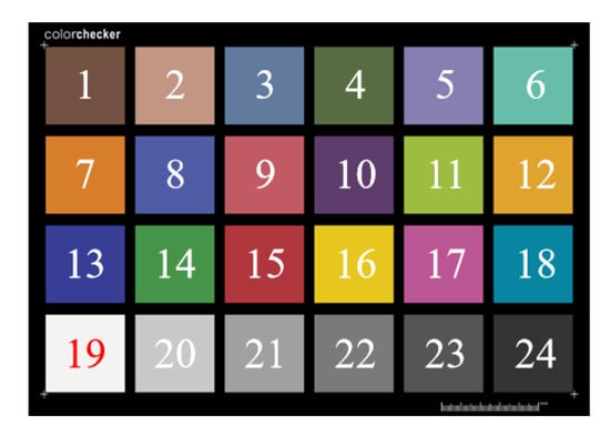
Figure 5.
X-Rite Color Checker Chart.
4. Results
To investigate the feasibility and accuracy of the color restoration that extracts color information from multispectral full-waveform data, the experimental datasets were utilized as described in Section 3.2. Since the waveform data measured by the FWMSL system is slightly asymmetrical with trailing, the measured data was fitted using both the proposed multispectral lognormal function and the Gaussian function [14] in order to verify whether the former can improve the color restoration accuracy compared to the latter. In addition, the intensity can be expressed as amplitude or integral area as mentioned in Section 3.1.1. This study aims to find the most suitable fitting method and intensity expression form to achieve the best effect of color restoration by comparing the four types of intensity, Gaussian amplitude, lognormal amplitude, Gaussian area and lognormal area. At the same time, this study also explores the optimal number of pulse accumulation in order to attenuate random errors and increase SNR of waveform data, thus improving the accuracy of color restoration finally.
We first test the FWMSL system under five different ambient light conditions including no light environment and four levels of light (Light 1, Light 2, Light 3 and Light 4) from weak to strong provided by the flashlight in order to validate the robustness of the color restoration method. 1000 echoes per channel per color square are recorded under the five lighting conditions. The probability density distributions of the standard deviation of background noise in RGB channels under different lighting conditions are shown in Figure 6.
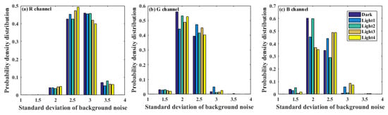
Figure 6.
Probability density distributions of the standard deviation of background noise in RGB channels under different ambient light conditions (Dark, Light 1, Light 2, Light 3 and Light 4) from weak to strong.
This histogram shows that the probability density distributions of the background noise of the G and B channels are more significantly affected by lighting conditions than the R channel. Regardless of whether ambient light is provided or not, the standard deviations of the background noise of the G and B channels are concentrated in the range of 2 to 2.5, which indicates that the influence of lighting conditions on the background noise is acceptable.
After analyzing the effects of ambient light, we further use the fixed point experimental data to determine the best type of intensity as well as the optimal number of pulse accumulation in order to avoid the impact of scanning on color restoration. The color restoration results in terms of RSD (relative standard deviation) at RGB channels by using the four types of intensity are displayed in Figure 7, which represents the stability of the retrieved color. Each sub-figure consists of color restoration results that vary with the number of accumulated pulses shown as different colored lines, which represent 24 colored squares of the color checker. In general, Figure 7 shows that the RSDs of color restoration results decrease with the number of pulse accumulation and gradually become stable.
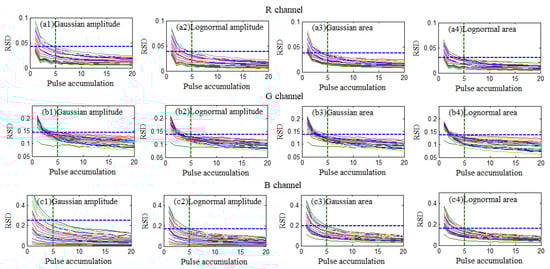
Figure 7.
Color restoration results in terms of the RSD (relative standard deviation) by using Gaussian amplitude, lognormal amplitude, Gaussian area and lognormal area with the number of accumulated pulses ranging from 1 to 20. The top row (a1–a4) depicts the results using the four types of intensity as input data at the R channel. The middle row (b1–b4) depicts the results using the four types of intensity as input data at the G channel. The bottom row (c1–c4) displays the results using the four types of intensity as input data at the B channel. Each sub-figure consists of color restoration results that vary with accumulated pulses shown as different colored lines. Different colored lines represent 24 colored squares of the color checker.
Comparing the subgraphs of each column in Figure 7, we find that the retrieved R values exhibit a higher stability (RSD = 0 ~ 0.1) (Figure 7a1–a4) than the retrieved B values (RSD = 0 ~ 0.5) (Figure 7c1–c4). This is attributed to the uneven distribution of the laser emission power (Figure 1a) as mentioned in Section 2, which results in a relatively low SNR for the B channel. Meanwhile, the RSD at R channel is reduced by 20% (Figure 7a3,a4) and the RSD at B channel is decreased from 0.2 to 0.16 (Figure 7c3,c4) using the lognormal function when number of pulse accumulation is 5. This result indicates that lognormal function is more suitable than Gaussian for the measured waveform data, offering higher color restoration stability and reliability.
Furthermore, in order to evaluate the color restoration accuracy, the correlation coefficient R2 between the retrieved RGB values and the corresponding true values are presented in Figure 8. This figure depicts a comparison among the color restoration results using the four types of intensity at each channel. Generally, R2 increases with the number of pulse accumulates and tends to stabilize until the accumulation number reaches 5.
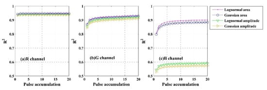
Figure 8.
Color restoration results in terms of R2 using Gaussian amplitude, lognormal amplitude, Gaussian area and lognormal area at R (a), G (b) and B (c) channels with the number of accumulated pulses ranging from 1 to 20. Each sub-figure consists of Gaussian amplitude, lognormal amplitude, Gaussian area and lognormal area with different splines. The dotted lines, circled lines, lower triangulated lines, right triangulated lines represent lognormal area, Gaussian area, lognormal amplitude and Gaussian amplitude, respectively.
Figure 8 exhibits that R2 is also affected by the SNR of each channel, so that the R channel performs higher accuracy than the B channel. Moreover, the results in RGB channels all evidence that the lognormal area has greater performance than the other three types of intensity according to the relatively high R2 about 0.9. Particularly, Figure 8 c displays that intensity expressed as integral area is significantly better than in amplitude, improving R2 from 0.6 to 0.9. Although the advantage of using the lognormal function is not obvious due to the small tail of the measured waveform, Figure 8c still shows that it improves the accuracy of B channel compared to Gaussian. Both Figure 7 and Figure 8 illustrate that the color restoration accuracy and the scanning efficiency can reach an optimal balance when the number of the pulse accumulation is 5. Additionally, in order to better compare the difference of the results using lognormal area with using the other intensity types, the corresponding results in Figure 7 and Figure 8 with 5 as the number of accumulated pulses are listed in Table 1 to display the color restoration performance in more detail.

Table 1.
Color restoration results using Gaussian amplitude, lognormal amplitude, Gaussian area and lognormal area with 5 as the number of accumulated pulses.
Table 1 displays color restoration results in terms of RSD and R2 at RGB channels with 5 as the number of accumulated pulses. The RSD values indicate that the lognormal area (R channel: 0.0304; B channel: 0.1596) has greater performance than the other three types of intensity (R channel: 0.0428, 0.0387, 0.0379; B channel: 0.2505, 0.1686, 0.1936), especially in R and B channels. Additionally, the R2 values shows that the color restoration accuracy in B channel can be greatly improved by using lognormal area (0.8865) compared with the others (0.5663, 0.5830 and 0.8706).
After evaluating the RGB values separately, the accuracy of the composite color is then assessed, which must meet the requirements of human eye recognition. Therefore, the term that represents the color difference is introduced to compare the retrieved color with the corresponding true color. The of 1.0 is the smallest color difference the human eye can distinguish. The of color restoration results using the four types of intensity with the pulse accumulation number of 5 are depicted in Figure 9.
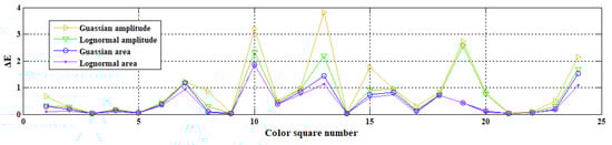
Figure 9.
Color restoration results in terms of using Gaussian amplitude, lognormal amplitude, Gaussian area and lognormal area with 5 as the number of accumulated pulses. The dotted lines, circled lines, lower triangulated lines, right triangulated lines represent Gaussian amplitude, lognormal amplitude, Gaussian area and lognormal area, respectively.
Figure 9 illustrates that the difference between the retrieved and true color of most squares are imperceptible when using lognormal area, while the results of other intensity types exceed the tolerance range of the human eyes. In order to visually observe the color difference, the retrieved colors using lognormal area with 5-pulse accumulation are presented in the CIE Luv space, as shown in Figure 10. The figure has 24 sub-figures in total. In each of them, the position of the center circle and the black scatters represent the true and retrieved colors, respectively. The sub-figures’ sizes are the same at 0.2 × 0.2. Thus, the color difference can be directly seen from the distance between the center and scatters as well as the background color.
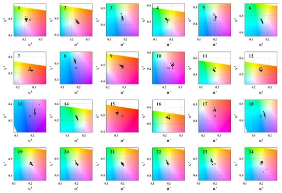
Figure 10.
Color restoration results in CIE using lognormal area with 5 as the number of accumulated pulses. Each sub-figure corresponds to a color square, its center is the true coordinate (u, v) of the color square and its size is 0.2 × 0.2.
Figure 10 displays that most of the color squares resemble their true colors based on the background color of the scatters and center point. Particularly, in the 8th, 10th and 15th sub-figures, despite the relatively far distance between the center and scatters, the background color looks similar. The previous results evidence the effectiveness of the color restoration method to extract color information from multispectral full-waveform data by using lognormal area with the pulse accumulation number of 5.
To further verify the color restoration performance of the proposed method on the scanned scene, the results using Gaussian and lognormal area with 5-pulse accumulation are both presented in Figure 11. Comparing with the point cloud colored by Gaussian area (Figure 11b), the color obtained with lognormal area (Figure 11c) visually overall looks much more close to the color checker (Figure 11a). Especially the color displayed in 2th, 4th, 7th, 9th, 12th and 16th squares have obvious improvement with lognormal area. Additionally, we can find that the 7th, 9th which have similar color display in Figure 11b, can be distinguished clearly in Figure 11c. The scanning results indicate the advantage in retrieving abundant colors for the asymmetric waveform.
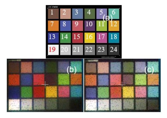
Figure 11.
(a) The color checker. (b) Point cloud colored using Gaussian area with 5-pulse accumulation. (c) Point cloud colored using lognormal area with 5-pulse accumulation.
After previous qualitative discussion, the colored point clouds are quantitatively compared with the actual color checker according to the RGB values and RSD. A total of 1000 points are randomly taken from each square to calculate the mean and RSD of the retrieved color values using Gaussian area (GA) and lognormal area (LA), as listed in Table 2. Table 2 illustrates the improvement in color information obtained by using lognormal area. Specifically, the retrieved RGB values of the 1th, 3th and 7th squares using lognormal area (R/G/B: 1th 137/106/88, 3th 129/148/166, 7th 214/113/65) are closer to the true values (R/G/B: 1th 115/82/68, 3th 98/122/157, 7th 214/126/44) compared with that using Gaussian area (R/G/B: 1th 68/88/110, 3th 98/122/157, 7th 180/54/21).
Table 2.
Quantitative analysis of the retrieved RGB values for the point cloud.
Table 2 also exhibits that the measured data has considerable higher accuracy in R channel than the other two channels according to RSD, which is related to the stability of color restoration. The RSD of the retrieved R values ranges from 0.83% to 3.61% while that of G and B values are over 10% in some squares. This metric also shows higher stability of the proposed method using lognormal area than Gaussian in color restoration. Additionally, the accuracy seems to be also related to the RGB values themselves, especially for the B channel. The accuracy of B channel is significant improved in the 19th square (B value: 242; RSD: GA 0.89, LA 0.75) compared with the 24th square ((B value: 52; RSD: GA 12.89, LA 11.37).
5. Discussion
This study proposed a theoretical model for color restoration using FWMSL measurements and verified the feasibility of the proposed method by utilizing the multispectral full-waveform data at RGB bands. This study is the first to establish a transformation model from high-sampling-rate multispectral waveform data to RGB values, thereby achieving the goal of obtaining color information only through active remote sensing without a camera. Previous studies have obtained the color values (R, G and B) by means of passive images [11,12,13]. Although these studies have achieved relatively high accuracy, geometric registration errors during active and passive fusion cannot be avoided, which needs considerable time and labor to compensate. Moreover, the image quality is affected by ambient light to a great extent, which will directly reduce the accuracy of the final color restoration results.
In this study, three main factors may limit the retrieval accuracy of the color information for FWMSL. First, the shape of the echo waveform is usually regarded as Gaussian, while data recorded by the FWMSL system is slightly asymmetric. Given that the measured waveform has a slight tailing, we assumed that the echo waveform conforms to the lognormal distribution and further proposed a multispectral lognormal function considering the spatial consistency between bands. In addition, for other multispectral LiDAR systems, if the shape of the measured waveform is different from that in this study, another suitable waveform fitting model should be selected accordingly to obtain accurate position and intensity information.
Secondly, the supercontinuum laser has extremely low output energy before 450 nm, near the blue band, which will cause color distortion to a certain extent. If the spectral information in the blue light region can be obtained through spectral simulation [21], the accuracy of color restoration will be improved.
Thirdly, this study analyzed the accuracy of color restoration under different pulse accumulations and provided the optimal number of pulse accumulation for color restoration. However, in practice, considering the scanning efficiency, the accuracy of color restoration is sometimes not optimal.
Further experiments involving extensive types of targets should be conducted with the FWMSL system to validate the performance of the system in acquiring the color information of different materials. The proposed theoretical model for color restoration should also be extended to other FWMSL systems and try to employ different waveform fitting models, such as Gaussian, generalized Gaussian or other custom models. The FWMSL system, with detectors covering a large wavelength range and full waveform recording of each channel may reveal more details about targets.
6. Conclusions
This study proposes a color restoration method for the FWMSL system, to extract color information from multispectral full-waveform data. An experimental dataset of 24-color standard color card measured by the FWMSL system. Results show that the current FWMSL system with three channels, which covers RGB bands, can restore the color information accurately.
The validation effort provided insights into several potential concerns of using multispectral full-waveform Lidar data to extract color information. First, lognormal function is more suitable to fit asymmetrical waveforms with trailing compared with Gaussian function, which helps to obtain waveform parameters more accurately, thus contributing to the accuracy of color restoration finally. The integral area is more stable than the amplitude and its intensity can significantly improve the accuracy of the color restoration. Based on the characteristics of the high-speed scanning of the LiDAR system, the SNR can be improved by accumulating pulses, thereby further improving the accuracy.
With the evaluation presented in this study, the color restoration method was proven feasible for retrieving color information from multispectral full-waveform data. The FWMSL application is not limited to the geometrical and physiological features of targets but it also extends to surface texture of targets. The FWMSL system provides great convenience for extracting target surface color information, which is beneficial to ecological, environmental and urban applications.
Author Contributions
Conceptualization, B.W. and S.S.; data curation, B.W.; formal analysis, B.W.; funding acquisition, S.S. and W.G.; investigation, X.C., D.H., Z.C. and X.L.; methodology, B.W.; project administration, S.S. and W.G.; resources, F.L.; supervision, S.S., W.G. and F.L.; writing—original draft, B.W.; writing—review & editing, S.S. and J.S. All authors have read and agreed to the published version of the manuscript.
Funding
This research was funded by National Key R&D Program of China, grant number 2018YFB0504500 and National Natural Science Foundation of China, grant number 41571370.
Acknowledgments
This work was supported by the National Key R&D Program of China (2018YFB0504500) and NSFC (41571370).
Conflicts of Interest
The authors declare no conflict of interest.
References
- Hancock, S.; Armston, J.; Li, Z.; Gaulton, R.; Lewis, P.; Disney, M.; Danson, F.M.; Strahler, A.; Schaaf, C.; Anderson, K.; et al. Waveform lidar over vegetation: An evaluation of inversion methods for estimating return energy. Remote Sens. Environ. 2015, 164, 208–224. [Google Scholar] [CrossRef]
- Wulder, M.A.; White, J.C.; Nelson, R.F. Lidar sampling for large-area forest characterization: A review. Remote Sens. Environ. 2012, 121, 196–209. [Google Scholar] [CrossRef]
- Wagner, W.; Ullrich, A.; Ducic, V.; Melzer, T.; Studnicka, N. Gaussian decomposition and calibration of a novel small-footprint full-waveform digitising airborne laser scanner. Isprs J. Photogramm. Remote Sens. 2006, 60, 100–112. [Google Scholar] [CrossRef]
- Pirotti, F. Analysis of full-waveform LiDAR data for forestry applications: a review of investigations and methods. Iforest-Biogeosciences For. 2011, 4, 100–106. [Google Scholar] [CrossRef]
- Liu, C.; Huang, H.; Gong, P.; Wang, X.; Wang, J.; Li, W.; Li, C.; Li, Z. Joint Use of ICESat/GLAS and Landsat Data in Land Cover Classification: A Case Study in Henan Province, China. IEEE J. Sel. Top. Appl. Earth Obs. Remote Sens. 2017, 8, 511–522. [Google Scholar] [CrossRef]
- Michelin, J.-C.; Mallet, C.; David, N. Building Edge Detection Using Small-Footprint Airborne Full-Waveform Lidar Data. In Proceedings of the XXII ISPRS Congress, Melbourne, Australia, 25 August–1 September 2012. [Google Scholar]
- Li, C.; Ma, L.; Zhou, M.; Zhu, X. Study on Road Detection Method from Full-Waveform LiDAR Data in Forested Area. In Proceedings of the Fourth International Conference on Ubiquitous Positioning, Shanghai, China, 3–4 November 2017. [Google Scholar]
- Nie, S.; Wang, C.; Dong, P.; Xi, X. Estimating Leaf Area Index of Maize Using Airborne Full-Waveform Lidar Data. Remote Sens. Lett. 2015, 7, 111–120. [Google Scholar] [CrossRef]
- Zhuang, W.; Mountrakis, G.; Weily, J.J., Jr.; Beier, C.M. Estimtio of above-ground forest biomass using metrics based on Gaussian decomposition of waveform lidar data. Int. J. Remote Sens. 2015, 36, 1871–1889. [Google Scholar] [CrossRef]
- Wang, H.; Glennie, C.; Prasad, S. Voxelization of Full Waveform LiDAR Data for Fusion with Hyperspectral Imagery. In Proceedings of the 2013 IEEE International Geoscience and Remote Sensing Symposium-IGARSS, Melbourne, Australia, 21–26 July 2013; pp. 3407–3410. [Google Scholar]
- Zheng, S.Y.; Huang, R.Y.; Zhou, Y. Registration of Optical Images with Lidar Data and Its Accuracy Assessment. Photogramm. Eng. Remote Sens. 2013, 79, 731–741. [Google Scholar] [CrossRef]
- Li, N.; Huang, X.; Zhang, F.; Wang, L. Registration of Aerial Imagery and Lidar Data in Desert Areas Using the Centroids of Bushes as Control Information. Photogramm. Eng. Remote Sens. 2013, 79, 743–752. [Google Scholar] [CrossRef]
- Moussa, W.; Abdel-Wahab, M.; Fritsch, D. An Automatic Procedure for Combining Digital Images and Laser Scanner Data. XXII ISPRS Congr. Tech. Comm. V 2012, 39-B5, 229–234. [Google Scholar] [CrossRef]
- Song, S.; Wang, B.; Gong, W.; Chen, Z.; Lin, X.; Sun, J.; Shi, S. A new waveform decomposition method for multispectral LiDAR. ISPRS J. Photogramm. Remote Sens. 2019, 149, 40–49. [Google Scholar] [CrossRef]
- Wei, G.; Shalei, S.; Bo, Z.; Shuo, S.; Faquan, L.; Xuewu, C. Multi-wavelength canopy LiDAR for remote sensing of vegetation: Design and system performance. ISPRS J. Photogramm. Remote Sens. 2012, 69, 1–9. [Google Scholar] [CrossRef]
- Hakala, T.; Suomalainen, J.; Kaasalainen, S.; Chen, Y. Full waveform hyperspectral LiDAR for terrestrial laser scanning. Opt. Express 2012, 20, 7119. [Google Scholar] [CrossRef] [PubMed]
- Woodhouse, I.H.; Nichol, C.; Sinclair, P.; Jack, J.; Morsdorf, F.; Malthus, T.J.; Patenaude, G. A Multispectral Canopy LiDAR Demonstrator Project. IEEE Geosci. Remote Sens. Lett. 2011, 8, 839–843. [Google Scholar] [CrossRef]
- Wallace, A.M.; McCarthy, A.; Nichol, C.; Ximing, R.; Morak, S.; Martinez-Ramirez, D.; Woodhouse, I.; Buller, G. Design and Evaluation of Multispectral LiDAR for the Recovery of Arboreal Parameters. IEEE Trans. Geosci. Remote Sens. 2014, 52, 4942–4954. [Google Scholar] [CrossRef]
- Malkamaki, T.; Kaasalainen, S.; Ilinca, J. Portable hyperspectral lidar utilizing 5 GHz multichannel full waveform digitization. Opt. Express 2019, 27, A468–A480. [Google Scholar] [CrossRef] [PubMed]
- Bretagne, E.; Dassonvalle, P.; Caron, G. Spherical target-based calibration of terrestrial laser scanner intensity. Application to colour information computation. ISPRS J. Photogramm. Remote Sens. 2018, 144, 14–27. [Google Scholar] [CrossRef]
- Chen, B.; Shi, S.; Gong, W.; Sun, J.; Chen, B.; Yang, L.D.J.; Guo, K.; Zhao, X. True-Color Three-Dimensional Imaging and Target Classification Based on Hyperspectral LiDAR. Remote Sens. 2019, 11, 1541. [Google Scholar] [CrossRef]
- Gunturk, B.K.; Glotzbach, J.; Altunbasak, Y.; Schafer, R.W.; Mersereau, R.M. Demosaicking: color filter array interpolation. IEEE Signal Process. Mag. 2005, 22, 44–54. [Google Scholar] [CrossRef]
- Li, X.; Gunturk, B.; Zhang, L. Image Demosaicing: A Systematic Survey. In Proceedings of the SPIE—The International Society for Optical Engineering, San Jose, CA, USA, 27–31 January 2008; 2008; p. 6822. [Google Scholar]
- Lin, Y.-C.; Mills, J.P.; Smith-Voysey, S. Rigorous pulse detection from full-waveform airborne laser scanning data. Int. J. Remote Sens. 2010, 31, 1303–1324. [Google Scholar] [CrossRef]
- Chauve, A.; Mallet, C.; Bretar, F.; Durrieu, S.; Pierrot-Deseilligny, M.; Puech, W. Processing full-waveform lidar data: modelling raw signals. Int. Arch. Photogramm. Remote Sens. Spat. Inf. Sci. 2008, 36, 102–107. [Google Scholar]
- Chauve, A.; Vega, C.; Durrieu, S.; Bretar, F.; Allouis, T.; Pierrot Deseilligny, M.; Puech, W. Advanced full-waveform lidar data echo detection: Assessing quality of derived terrain and tree height models in an alpine coniferous forest. Int. J. Remote Sens. 2009, 30, 5211–5228. [Google Scholar] [CrossRef]
- Jutzi, B.; Stilla, U. Range determination with waveform recording laser systems using a Wiener Filter. ISPRS J. Photogramm. Remote Sens. 2006, 61, 95–107. [Google Scholar] [CrossRef]
- Li, X.; Xu, X.; Xu, L. Within-footprint roughness measurements using ICESat/GLAS waveform and LVIS elevation. Meas. Sci. Technol. 2016, 27, 125012. [Google Scholar] [CrossRef]
- Plataniotis, K.N.; Venetsanopoulos, A.N. Color Image Processing and Applications 2013; Springer Science & Business Media: Berlin, Germany, 2013. [Google Scholar]
© 2020 by the authors. Licensee MDPI, Basel, Switzerland. This article is an open access article distributed under the terms and conditions of the Creative Commons Attribution (CC BY) license (http://creativecommons.org/licenses/by/4.0/).