Simulating the Impact of Urban Surface Evapotranspiration on the Urban Heat Island Effect Using the Modified RS-PM Model: A Case Study of Xuzhou, China


Abstract

1. Introduction
2. Material and Methods
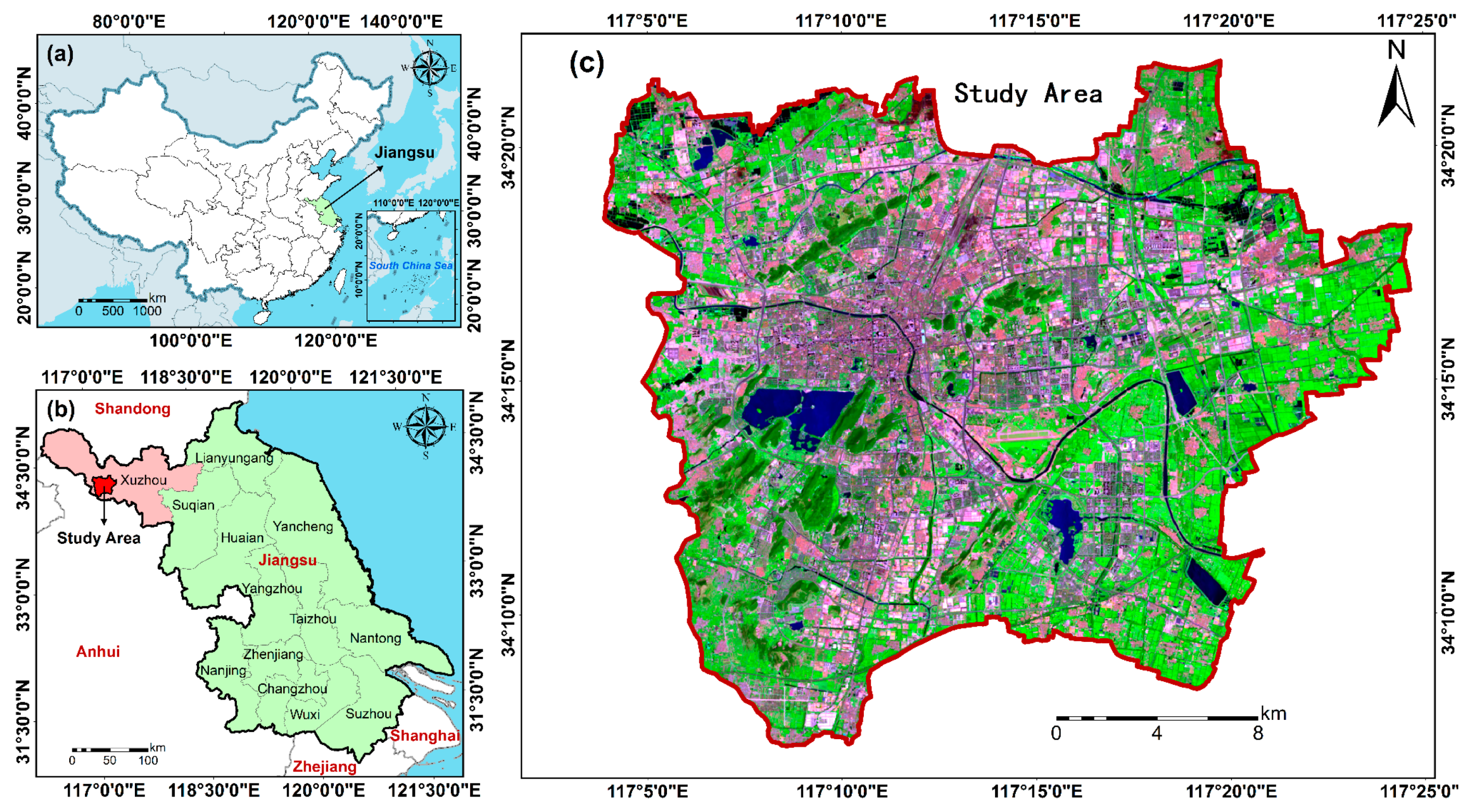
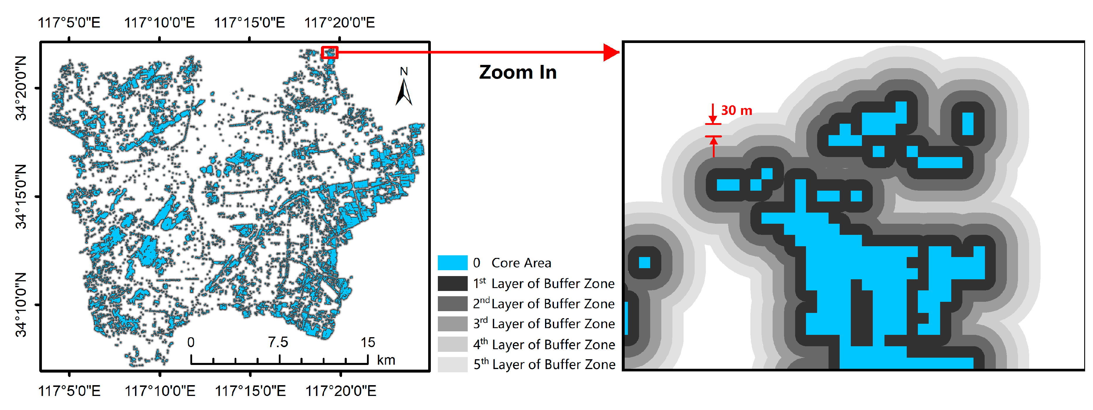
2.1. Study Area
2.2. Data
2.2.1. Satellite Data
2.2.2. Meteorological Observations
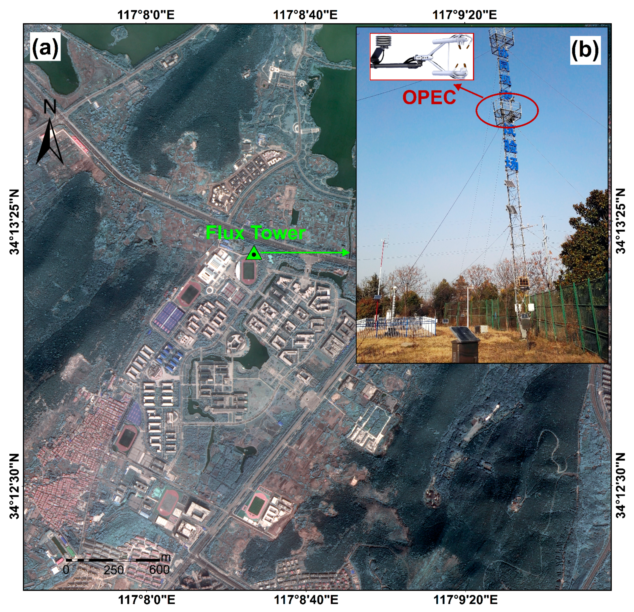
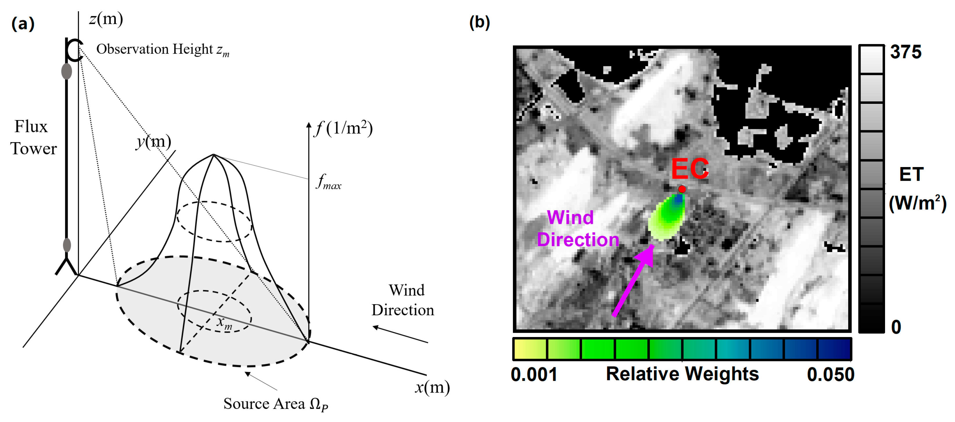
2.2.3. Flux Observations
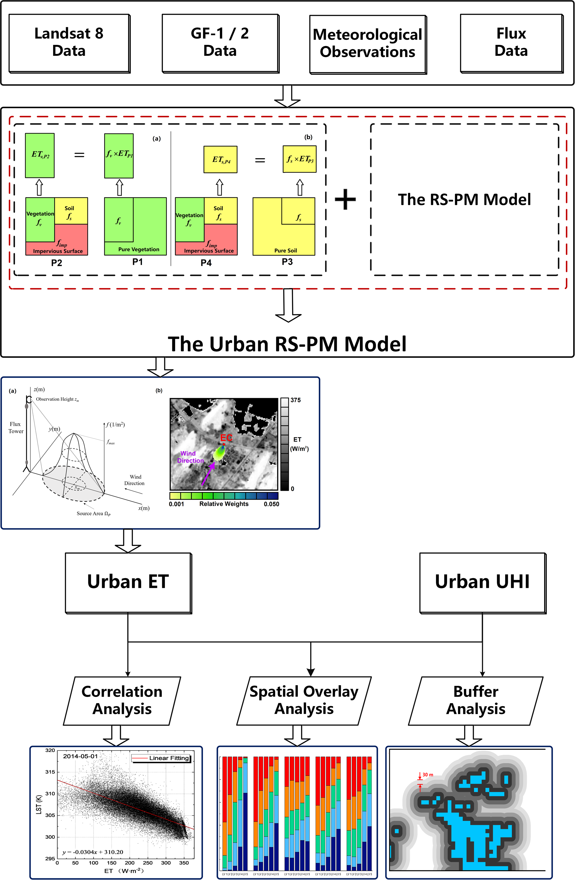
2.3. ET Estimation Using the Urban RS-PM Model
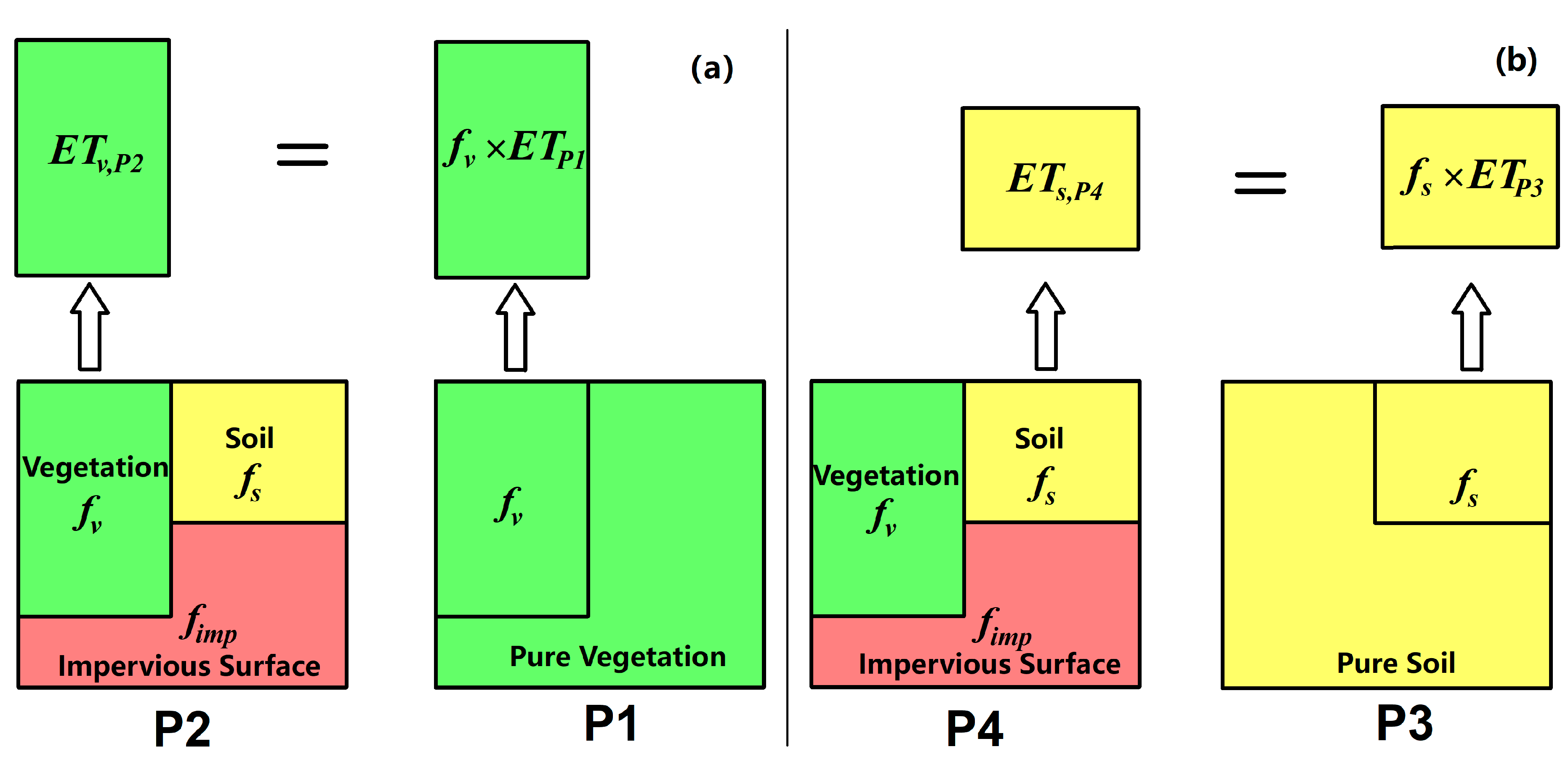
2.3.1. Linear Spectral Analysis
2.3.2. Component Net Radiation Inversion
2.3.3. Component Aerodynamic Resistance Inversion
2.3.4. Component Surface Resistance Inversion
2.3.5. Soil Heat Flux Inversion
2.4. Land Surface Temperature Inversion Using the IMW Algorithm
3. Results
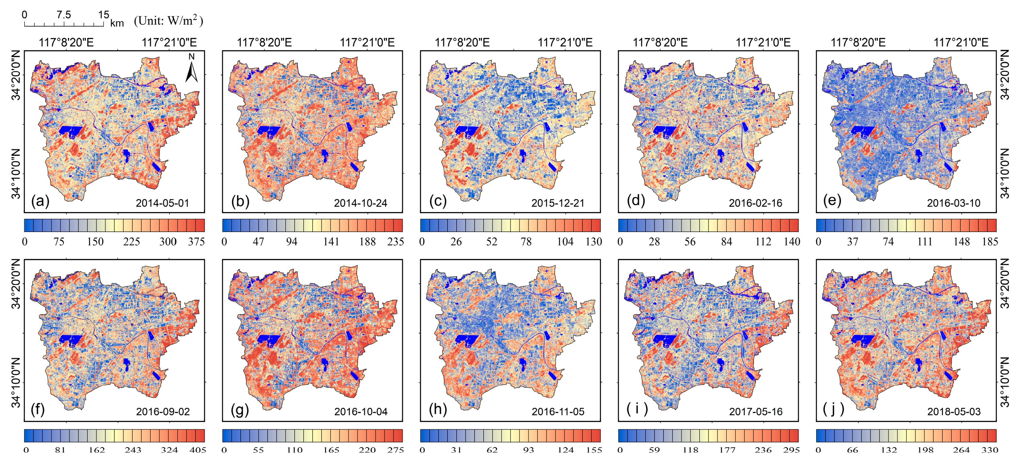
3.1. Urban ET
3.1.1. Urban RS-PM Model Estimates
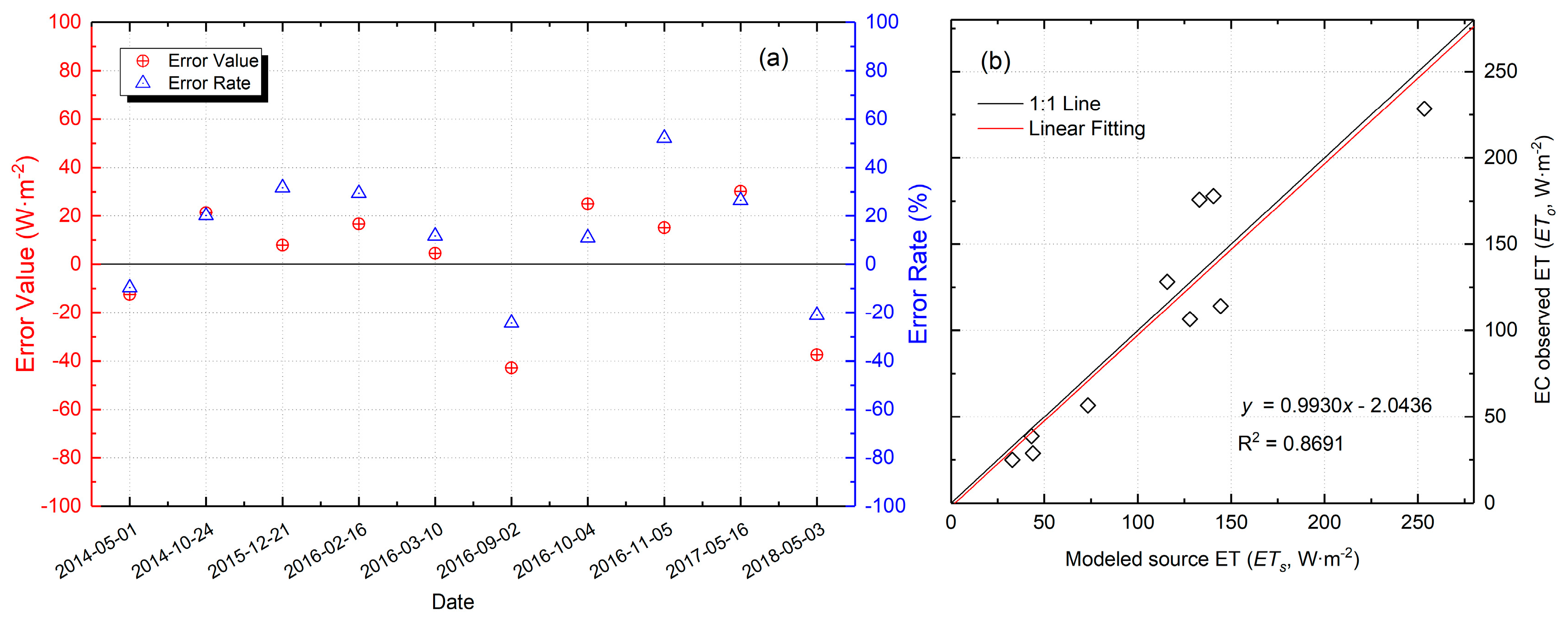
3.1.2. Accuracy of Modeled ET
3.2. ET Effects on the UHI
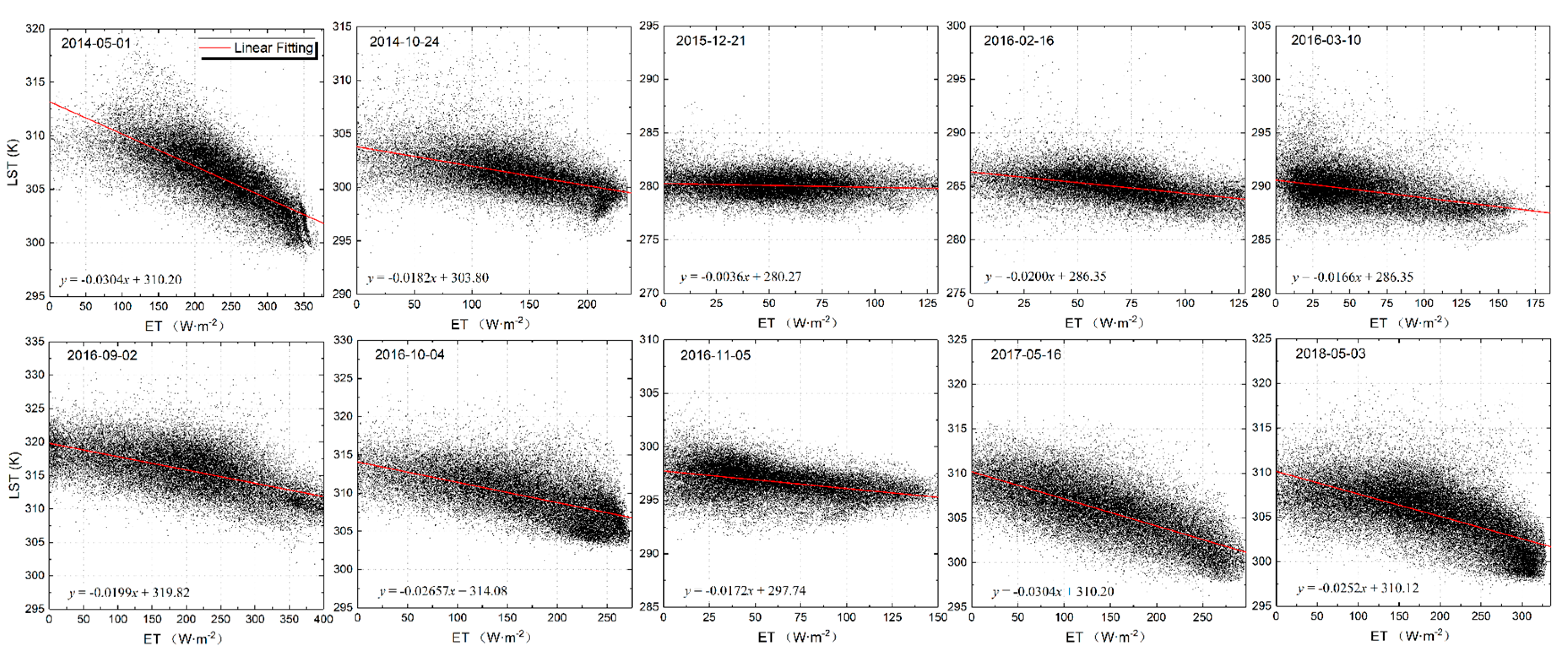
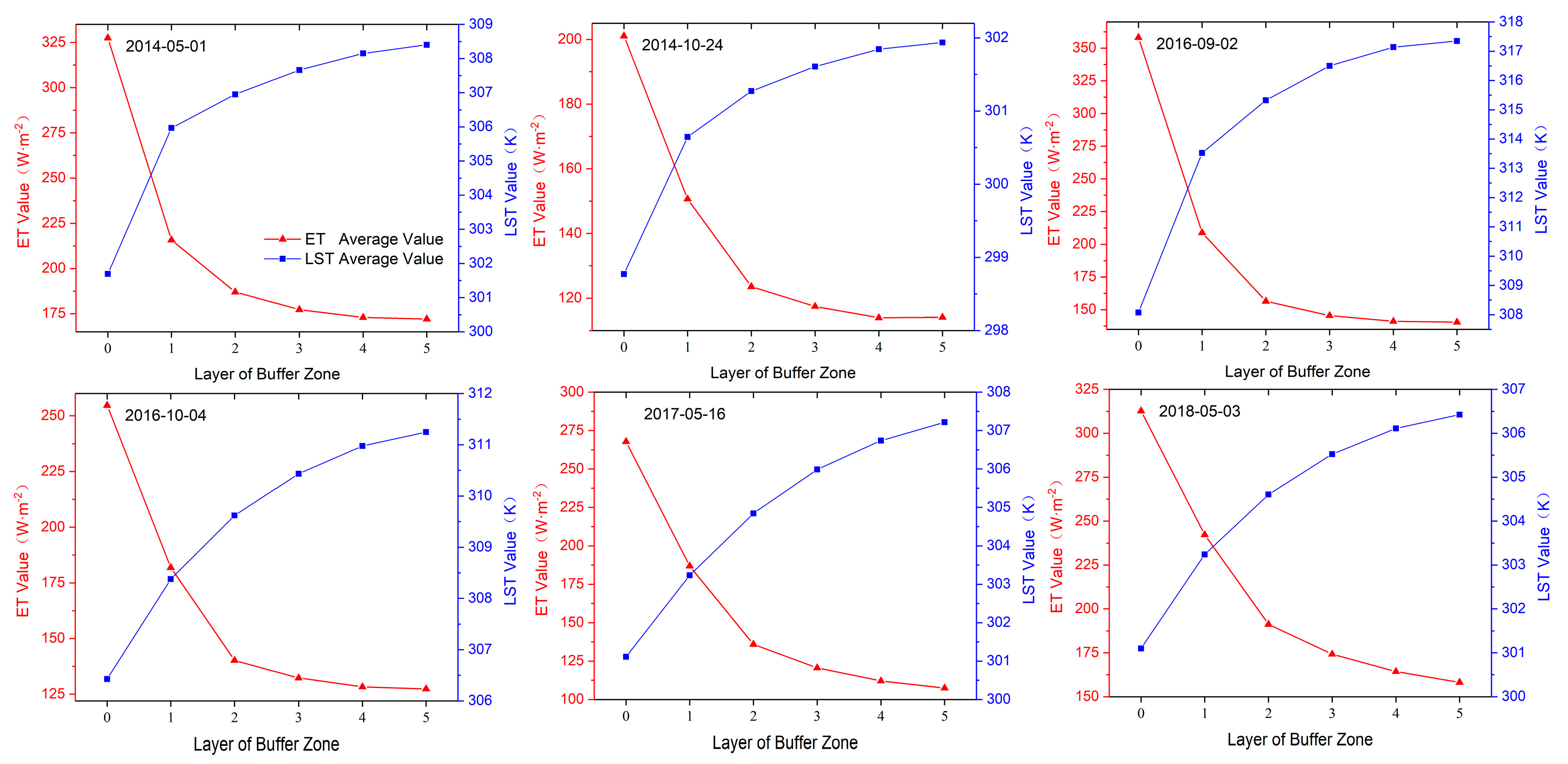
3.2.1. Relationship between Urban ET and LST
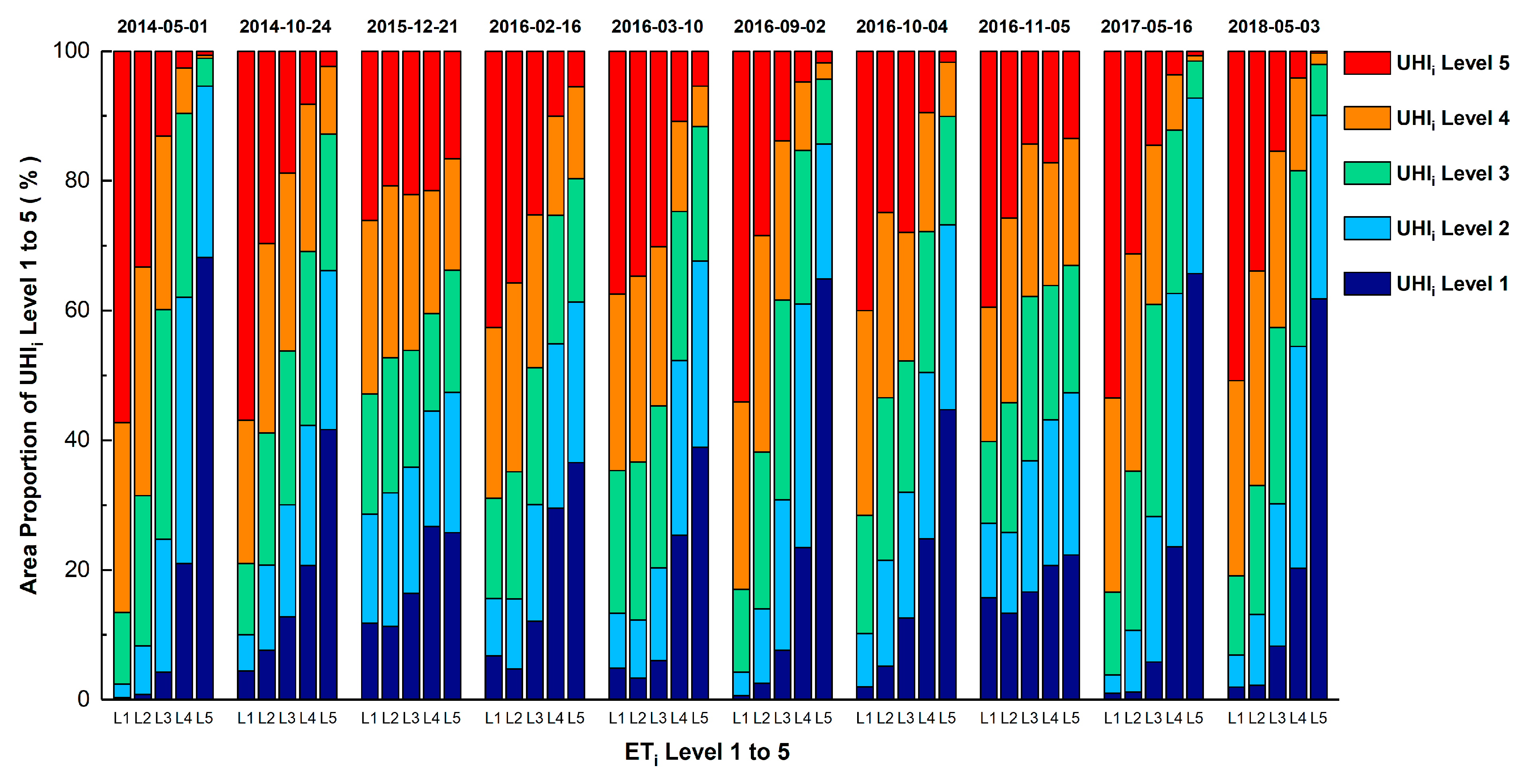
3.2.2. Relationship between the Intensity of Urban ET and the UHI Effect
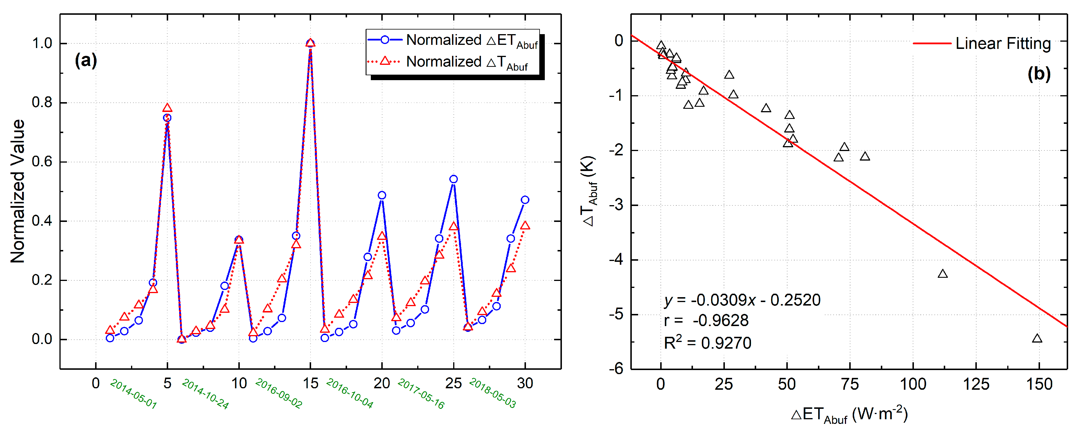
3.2.3. The Effect of High ET Intensity on UHI
4. Discussion
5. Conclusions
Author Contributions
Funding
Acknowledgments
Conflicts of Interest
References
- Taha, H. Urban climates and heat islands: Albedo, evapotranspiration, and anthropogenic heat. Energy Build. 1997, 25, 99–103. [Google Scholar] [CrossRef]
- Lu, L.; Weng, Q.; Guo, H.; Feng, S.; Li, Q. Assessment of urban environmental change using multi-source remote sensing time series (2000–2016): A comparative analysis in selected megacities in Eurasia. Sci. Total Environ. 2019, 684, 567–577. [Google Scholar] [CrossRef] [PubMed]
- Li, L.; Tan, Y.; Ying, S.; Yu, Z.; Li, Z.; Lan, H. Impact of land cover and population density on land surface temperature: Case study in Wuhan, China. J. Appl. Remote Sens. 2014, 8, 084993. [Google Scholar] [CrossRef]
- Peng, S.; Piao, S.; Ciais, P.; Friedlingstein, P.; Ottle, C.; Bréon, F.-M.; Nan, H.; Zhou, L.; Myneni, R.B. Surface Urban Heat Island Across 419 Global Big Cities. Environ. Sci. Technol. 2012, 46, 696–703. [Google Scholar] [CrossRef]
- Manoli, G.; Fatichi, S.; Schläpfer, M.; Yu, K.; Crowther, T.W.; Meili, N.; Burlando, P.; Katul, G.G.; Bou-Zeid, E. Magnitude of urban heat islands largely explained by climate and population. Nature 2019, 573, 55–60. [Google Scholar] [CrossRef]
- Du, H.; Cai, W.; Xu, Y.; Wang, Z.; Wang, Y.; Cai, Y. Quantifying the cool island effects of urban green spaces using remote sensing Data. Urban For. Urban Green. 2017, 27, 24–31. [Google Scholar] [CrossRef]
- Arnfield, A.J. Two decades of urban climate research: A review of turbulence, exchanges of energy and water, and the urban heat island. Int. J. Climatol. 2003, 23, 1–26. [Google Scholar] [CrossRef]
- Feizizadeh, B.; Blaschke, T. Examining Urban Heat Island Relations to Land Use and Air Pollution: Multiple Endmember Spectral Mixture Analysis for Thermal Remote Sensing. IEEE J. Sel. Top. Appl. Earth Obs. Remote Sens. 2013, 6, 1749–1756. [Google Scholar] [CrossRef]
- Shashua-Bar, L.; Pearlmutter, D.; Erell, E. The cooling efficiency of urban landscape strategies in a hot dry climate. Landsc. Urban Plan. 2009, 92, 179–186. [Google Scholar] [CrossRef]
- Hamada, S.; Ohta, T. Seasonal variations in the cooling effect of urban green areas on surrounding urban areas. Urban For. Urban Green. 2010, 9, 15–24. [Google Scholar] [CrossRef]
- Rahman, M.A.; Moser, A.; Rötzer, T.; Pauleit, S. Within canopy temperature differences and cooling ability of Tilia cordata trees grown in urban conditions. Build. Environ. 2017, 114, 118–128. [Google Scholar] [CrossRef]
- Chow, W.T.L.; Brennan, D.; Brazel, A.J. Urban Heat Island Research in Phoenix, Arizona: Theoretical Contributions and Policy Applications. Bull. Am. Meteorol. Soc. 2012, 93, 517–530. [Google Scholar] [CrossRef]
- Oliveira, S.; Andrade, H.; Vaz, T. The cooling effect of green spaces as a contribution to the mitigation of urban heat: A case study in Lisbon. Build. Environ. 2011, 46, 2186–2194. [Google Scholar] [CrossRef]
- Georgi, J.N.; Dimitriou, D. The contribution of urban green spaces to the improvement of environment in cities: Case study of Chania, Greece. Build. Environ. 2010, 45, 1401–1414. [Google Scholar] [CrossRef]
- Cheung, P.K.; Jim, C.Y. Comparing the cooling effects of a tree and a concrete shelter using PET and UTCI. Build. Environ. 2018, 130, 49–61. [Google Scholar] [CrossRef]
- Fung, C.K.W.; Jim, C.Y. Microclimatic resilience of subtropical woodlands and urban-forest benefits. Urban For. Urban Green. 2019, 42, 100–112. [Google Scholar] [CrossRef]
- Lo, C.P.; Quattrochi, D.A. Land-Use and Land-Cover Change, Urban Heat Island Phenomenon, and Health Implications. Photogramm. Eng. Remote Sens. 2003, 69, 1053–1063. [Google Scholar] [CrossRef]
- Gallo, K.P.; McNab, A.L.; Karl, T.R.; Brown, J.F.; Hood, J.J.; Tarpley, J.D. The use of a vegetation index for assessment of the urban heat island effect. Int. J. Remote Sens. 1993, 14, 2223–2230. [Google Scholar] [CrossRef]
- Weng, Q.; Lu, D.; Schubring, J. Estimation of land surface temperature-vegetation abundance relationship for urban heat island studies. Remote Sens. Environ. 2004, 89, 467–483. [Google Scholar] [CrossRef]
- Fintikakis, N.; Gaitani, N.; Santamouris, M.; Assimakopoulos, M.; Assimakopoulos, D.N.; Fintikaki, M.; Albanis, G.; Papadimitriou, K.; Chryssochoides, E.; Katopodi, K.; et al. Bioclimatic design of open public spaces in the historic centre of Tirana, Albania. Sustain. Cities Soc. 2011, 1, 54–62. [Google Scholar] [CrossRef]
- Cao, X.; Onishi, A.; Chen, J.; Imura, H. Quantifying the cool island intensity of urban parks using ASTER and IKONOS data. Landsc. Urban Plan. 2010, 96, 224–231. [Google Scholar] [CrossRef]
- Rahman, M.A.; Armson, D.; Ennos, A.R. A comparison of the growth and cooling effectiveness of five commonly planted urban tree species. Urban Ecosyst. 2015, 18, 371–389. [Google Scholar] [CrossRef]
- Evju, M.; Sverdrup-Thygeson, A. Spatial configuration matters: A test of the habitat amount hypothesis for plants in calcareous grasslands. Landsc. Ecol. 2016, 31, 1891–1902. [Google Scholar] [CrossRef]
- Zhou, W.; Huang, G.; Cadenasso, M.L. Does spatial configuration matter? Understanding the effects of land cover pattern on land surface temperature in urban landscapes. Landsc. Urban Plan. 2011, 102, 54–63. [Google Scholar] [CrossRef]
- Boegh, E.; Soegaard, H.; Hanan, N.; Kabat, P.; Lesch, L. A Remote Sensing Study of the NDVI–Ts Relationship and the Transpiration from Sparse Vegetation in the Sahel Based on High-Resolution Satellite Data. Remote Sens. Environ. 1999, 69, 224–240. [Google Scholar] [CrossRef]
- Mu, Q.; Heinsch, F.A.; Zhao, M.; Running, S.W. Development of a global evapotranspiration algorithm based on MODIS and global meteorology data. Remote Sens. Environ. 2007, 111, 519–536. [Google Scholar] [CrossRef]
- Pataki, D.E.; McCarthy, H.R.; Litvak, E.; Pincetl, S. Transpiration of urban forests in the Los Angeles metropolitan area. Ecol. Appl. 2011, 21, 661–677. [Google Scholar] [CrossRef]
- Peters, E.B.; Hiller, R.V.; McFadden, J.P. Seasonal contributions of vegetation types to suburban evapotranspiration. J. Geophys. Res. 2011, 116, G01003. [Google Scholar] [CrossRef]
- Wang, C.; Yang, J.; Myint, S.W.; Wang, Z.-H.; Tong, B. Empirical modeling and spatio-temporal patterns of urban evapotranspiration for the Phoenix metropolitan area, Arizona. GIScience Remote Sens. 2016, 53, 778–792. [Google Scholar] [CrossRef]
- Vahmani, P.; Hogue, T.S. High-resolution land surface modeling utilizing remote sensing parameters and the Noah UCM: A case study in the Los Angeles Basin. Hydrol. Earth Syst. Sci. 2014, 18, 4791–4806. [Google Scholar] [CrossRef]
- Vahmani, P.; Hogue, T.S. Incorporating an Urban Irrigation Module into the Noah Land Surface Model Coupled with an Urban Canopy Model. J. Hydrometeorol. 2014, 15, 1440–1456. [Google Scholar] [CrossRef]
- Mu, Q.; Zhao, M.; Running, S.W. Improvements to a MODIS global terrestrial evapotranspiration algorithm. Remote Sens. Environ. 2011, 115, 1781–1800. [Google Scholar] [CrossRef]
- Zhang, Y.; Li, L.; Chen, L.; Liao, Z.; Wang, Y.; Wang, B.; Yang, X. A Modified Multi-Source Parallel Model for Estimating Urban Surface Evapotranspiration Based on ASTER Thermal Infrared Data. Remote Sens. 2017, 9, 1029. [Google Scholar] [CrossRef]
- NASA Jet Propulsion Laboratory. Available online: https://asterweb.jpl.nasa.gov/swir-alert.asp (accessed on 15 September 2019).
- Zhang, Y.; Li, L.; Qin, K.; Wang, Y.; Chen, L.; Yang, X. Remote sensing estimation of urban surface evapotranspiration based on a modified Penman–Monteith model. J. Appl. Remote Sens. 2018, 12, 1. [Google Scholar] [CrossRef]
- Cleugh, H.A.; Leuning, R.; Mu, Q.; Running, S.W. Regional evaporation estimates from flux tower and MODIS satellite data. Remote Sens. Environ. 2007, 106, 285–304. [Google Scholar] [CrossRef]
- Sheffield, J.; Wood, E.F.; Munoz-Arriola, F. Long-Term Regional Estimates of Evapotranspiration for Mexico Based on Downscaled ISCCP Data. J. Hydrometeorol. 2010, 11, 253–275. [Google Scholar] [CrossRef]
- Hu, G.; Jia, L.; Menenti, M. Comparison of MOD16 and LSA-SAF MSG evapotranspiration products over Europe for 2011. Remote Sens. Environ. 2015, 156, 510–526. [Google Scholar] [CrossRef]
- He, M.; Kimball, J.S.; Yi, Y.; Running, S.W.; Guan, K.; Moreno, A.; Wu, X.; Maneta, M. Satellite data-driven modeling of field scale evapotranspiration in croplands using the MOD16 algorithm framework. Remote Sens. Environ. 2019, 230, 111201. [Google Scholar] [CrossRef]
- Xuzhou Bureau of Statistics Xuzhou Statistical Yearbook 2018; China Statistics Press: Beijing, China, 2018.
- RIDD, M.K. Exploring a V-I-S (vegetation-impervious surface-soil) model for urban ecosystem analysis through remote sensing: Comparative anatomy for cities†. Int. J. Remote Sens. 1995, 16, 2165–2185. [Google Scholar] [CrossRef]
- Wu, C. Normalized spectral mixture analysis for monitoring urban composition using ETM+ imagery. Remote Sens. Environ. 2004, 93, 480–492. [Google Scholar] [CrossRef]
- Rivas, R.; Caselles, V. A simplified equation to estimate spatial reference evaporation from remote sensing-based surface temperature and local meteorological data. Remote Sens. Environ. 2004, 93, 68–76. [Google Scholar] [CrossRef]
- Liang, S. Narrowband to broadband conversions of land surface albedo I Algorithms. Remote Sens. Environ. 2001, 76, 213–238. [Google Scholar] [CrossRef]
- Qin, Z.; Karnieli, A.; Berliner, P. A mono-window algorithm for retrieving land surface temperature from Landsat TM data and its application to the Israel-Egypt border region. Int. J. Remote Sens. 2001, 22, 3719–3746. [Google Scholar] [CrossRef]
- Long, D.; Singh, V.P. A Two-source Trapezoid Model for Evapotranspiration (TTME) from satellite imagery. Remote Sens. Environ. 2012, 121, 370–388. [Google Scholar] [CrossRef]
- Long, D.; Singh, V.P. Integration of the GG model with SEBAL to produce time series of evapotranspiration of high spatial resolution at watershed scales. J. Geophys. Res. 2010, 115, D21128. [Google Scholar] [CrossRef]
- Spencer, J.W. Fourier series representation of the position of the sun. Search 1971, 2, 172. [Google Scholar]
- Wong, L.T.; Chow, W.K. Solar radiation model. Appl. Energy 2001, 69, 191–224. [Google Scholar] [CrossRef]
- Brutsaert, W. On a derivable formula for long-wave radiation from clear skies. Water Resour. Res. 1975, 11, 742–744. [Google Scholar] [CrossRef]
- Mao, K.; Qin, Z.; Shi, J.; Gong, P. A practical split-window algorithm for retrieving land-surface temperature from MODIS data. Int. J. Remote Sens. 2005, 26, 3181–3204. [Google Scholar] [CrossRef]
- Kustas, W.P.; Norman, J.M. Evaluation of soil and vegetation heat flux predictions using a simple two-source model with radiometric temperatures for partial canopy cover. Agric. For. Meteorol. 1999, 94, 13–29. [Google Scholar] [CrossRef]
- Kanda, M.; Kanega, M.; Kawai, T.; Moriwaki, R.; Sugawara, H. Roughness lengths for momentum and heat derived from outdoor urban scale models. J. Appl. Meteorol. Climatol. 2007, 46, 1067–1079. [Google Scholar] [CrossRef]
- Brutsaert, W. Evaporation into the Atmosphere: Theory, History and Applications; Springer: Dordrecht, The Netherlands, 1982; ISBN 978-90-481-8365-4. [Google Scholar]
- Kustas, W.P.; Choudhury, B.J.; Moran, M.S.; Reginato, R.J.; Jackson, R.D.; Gay, L.W.; Weaver, H.L. Determination of sensible heat flux over sparse canopy using thermal infrared data. Agric. For. Meteorol. 1989, 44, 197–216. [Google Scholar] [CrossRef]
- Choudhury, B.J.; Reginato, R.J.; Idso, S.B. An analysis of infrared temperature observations over wheat and calculation of latent heat flux. Agric. For. Meteorol. 1986, 37, 75–88. [Google Scholar] [CrossRef]
- Choudhury, B.J.; Monteith, J.L. A four-layer model for the heat budget of homogeneous land surfaces. Q. J. R. Meteorol. Soc. 1988, 114, 373–398. [Google Scholar] [CrossRef]
- Liu, S.; Lu, L.; Mao, D.; Jia, L. Evaluating parameterizations of aerodynamic resistance to heat transfer using field measurements. Hydrol. Earth Syst. Sci. 2007, 11, 769–783. [Google Scholar] [CrossRef]
- Level 1 and Atmosphere Archive & Distribution System Distributed Active Archive Center (LAADS DAAC). Available online: https://ladsweb.modaps.eosdis.nasa.gov/search/order/1/MOD15A2H (accessed on 13 October 2019).
- Leuning, R.; Zhang, Y.Q.; Rajaud, A.; Cleugh, H.; Tu, K. A simple surface conductance model to estimate regional evaporation using MODIS leaf area index and the Penman-Monteith equation. Water Resour. Res. 2008, 44, W10419. [Google Scholar] [CrossRef]
- Wallace, J.S.; Holwill, C.J. Soil evaporation from tiger-bush in south-west Niger. J. Hydrol. 1997, 188–189, 188–189. [Google Scholar] [CrossRef]
- Friedl, M.A. Relationships among remotely sensed data, surface energy balance, and area-averaged fluxes over partially vegetated land surfaces. J. Appl. Meteorol. 1996, 35, 2091–2103. [Google Scholar] [CrossRef]
- Qin, Z.; Dall, G.; Karni, A.; Berliner, P. Derivation of split window algorithm and its sensitivity analysis for retrieving land surface temperature from NOAA-advanced very high resolution radiometer data. J. Geophys. Res. 2001, 106, 22655–22670. [Google Scholar] [CrossRef]
- Rozenstein, O.; Qin, Z.; Derimian, Y.; Karnieli, A. Derivation of land surface temperature for landsat-8 TIRS using a split window algorithm. Sensors (Switzerland) 2014, 14, 5768–5780. [Google Scholar] [CrossRef]
- Jiménez-Muñoz, J.C.; Sobrino, J.A.; Skokovic, D.; Mattar, C.; Cristobal, J. Land surface temperature retrieval methods from Landsat-8 thermal infrared sensor data. Geosci. Remote Sens. Lett. IEEE 2014, 11, 1840–1843. [Google Scholar] [CrossRef]
- Wang, F.; Qin, Z.; Song, C.; Tu, L.; Karnieli, A.; Zhao, S. An Improved Mono-Window Algorithm for Land Surface Temperature Retrieval from Landsat 8 Thermal Infrared Sensor Data. Remote Sens. 2015, 7, 4268–4289. [Google Scholar] [CrossRef]
- Brunsell, N.A.; Ham, J.M.; Arnold, K.A. Validating remotely sensed land surface fluxes in heterogeneous terrain with large aperture scintillometry. Int. J. Remote Sens. 2011, 32, 6295–6314. [Google Scholar] [CrossRef]
- Kleissl, J.; Hong, S.-H.; Hendrickx, J.M.H. New Mexico Scintillometer Network: Supporting Remote Sensing and Hydrologic and Meteorological Models. Bull. Am. Meteorol. Soc. 2009, 90, 207–218. [Google Scholar] [CrossRef]
- Wang, Y.-C.; Bian, Z.-F.; Qin, K.; Zhang, Y.; Lei, S.-G. A modified building energy model coupled with urban parameterization for estimating anthropogenic heat in urban areas. Energy Build. 2019, 202, 109377. [Google Scholar] [CrossRef]
- Schmid, H.P. Footprint modeling for vegetation atmosphere exchange studies: A review and perspective. Agric. For. Meteorol. 2002, 113, 159–183. [Google Scholar] [CrossRef]
- Li, J.; Song, C.; Cao, L.; Zhu, F.; Meng, X.; Wu, J. Impacts of landscape structure on surface urban heat islands: A case study of Shanghai, China. Remote Sens. Environ. 2011, 115, 3249–3263. [Google Scholar] [CrossRef]
- Zhang, Y.; Odeh, I.O.A.; Ramadan, E. Assessment of land surface temperature in relation to landscape metrics and fractional vegetation cover in an urban/peri-urban region using Landsat data. Int. J. Remote Sens. 2013, 34, 168–189. [Google Scholar] [CrossRef]
- Spronken-Smith, R.A.; Oke, T.R. The thermal regime of urban parks in two cities with different summer climates. Int. J. Remote Sens. 1998, 19, 2085–2104. [Google Scholar] [CrossRef]
- Upmanis, H.; Eliasson, I.; Lindqvist, S. The influence of green areas on nocturnal temperatures in a high latitude city (Göteborg, Sweden). Int. J. Climatol. 1998, 18, 681–700. [Google Scholar] [CrossRef]
- Chang, C.-R.; Li, M.-H.; Chang, S.-D. A preliminary study on the local cool-island intensity of Taipei city parks. Landsc. Urban Plan. 2007, 80, 386–395. [Google Scholar] [CrossRef]
- Zhang, Y.; Chen, L.; Wang, Y.; Chen, L.; Yao, F.; Wu, P.; Wang, B.; Li, Y.; Zhou, T.; Zhang, T. Research on the Contribution of Urban Land Surface Moisture to the Alleviation Effect of Urban Land Surface Heat Based on Landsat 8 Data. Remote Sens. 2015, 7, 10737–10762. [Google Scholar] [CrossRef]
- Morakinyo, T.E.; Kong, L.; Lau, K.K.L.; Yuan, C.; Ng, E. A study on the impact of shadow-cast and tree species on in-canyon and neighborhood’s thermal comfort. Build. Environ. 2017, 115, 1–17. [Google Scholar] [CrossRef]
- Tan, C.L.; Wong, N.H.; Jusuf, S.K. Outdoor mean radiant temperature estimation in the tropical urban environment. Build. Environ. 2013, 64, 118–129. [Google Scholar] [CrossRef]
- Yan, C.; Guo, Q.; Li, H.; Li, L.; Qiu, G.Y. Quantifying the cooling effect of urban vegetation by mobile traverse method: A local-scale urban heat island study in a subtropical megacity. Build. Environ. 2020, 169, 106541. [Google Scholar] [CrossRef]
- Doick, K.J.; Peace, A.; Hutchings, T.R. The role of one large greenspace in mitigating London’s nocturnal urban heat island. Sci. Total Environ. 2014, 493, 662–671. [Google Scholar] [CrossRef]
- Feyisa, G.L.; Dons, K.; Meilby, H. Efficiency of parks in mitigating urban heat island effect: An example from Addis Ababa. Landsc. Urban Plan. 2014, 123, 87–95. [Google Scholar] [CrossRef]
- Lin, W.; Yu, T.; Chang, X.; Wu, W.; Zhang, Y. Calculating cooling extents of green parks using remote sensing: Method and test. Landsc. Urban Plan. 2015, 134, 66–75. [Google Scholar] [CrossRef]
- Yang, C.; He, X.; Yu, L.; Yang, J.; Yan, F.; Bu, K.; Chang, L.; Zhang, S. The Cooling Effect of Urban Parks and Its Monthly Variations in a Snow Climate City. Remote Sens. 2017, 9, 1066. [Google Scholar] [CrossRef]


| Sensor | Resolution | Scene ID | Acquisition Date | Cold or Warm Season | Acquisition Time (GMT) |
|---|---|---|---|---|---|
| Landsat 8 | OLI Band: 30 m TIRS Band: 100 m | LC81210362014121LGN00 | 01–05–2014 | Warm | 02:42:29 |
| LC81210362014297LGN00 | 24–10–2014 | Warm | 02:42:58 | ||
| LC81220362015355LGN00 | 21–12–2015 | Cold | 02:49:04 | ||
| LC81210362016047LGN01 | 16–02–2016 | Cold | 02:42:40 | ||
| LC81220362016070LGN01 | 10–03–2016 | Cold | 02:48:47 | ||
| LC81220362016246LGN00 | 02–09–2016 | Warm | 02:49:07 | ||
| LC81220362016278LGN00 | 04–10–2016 | Warm | 02:49:11 | ||
| LC81220362016310LGN00 | 05–11–2016 | Cold | 02:49:16 | ||
| LC81220362017136LGN00 | 16–05–2017 | Warm | 02:48:22 | ||
| LC81220362018123LGN00 | 03–05–2018 | Warm | 02:48:04 | ||
| GF-1 | PAN Band: 2 m MS Band: 8 m | 579791 | 24–10–2014 | 03:26:39 | |
| 579790 | 24–10–2014 | 03:26:34 | |||
| GF-2 | PAN Band: 1 m MS Band: 4 m | 2872975 | 05–10–2016 | 03:25:48 |
| Date | Recording Time (GMT) | Air Temperature (K) | Wind Speed (m/s) | Atmospheric Pressure (kPa) | Air Relative Humidity (%) | Water Vapor Pressure (hPa) |
|---|---|---|---|---|---|---|
| 01–05–2014 | 02:30:00 | 297.42 | 2.66 | 101.12 | 55.12 | 16.70 |
| 24–10–2014 | 02:30:00 | 293.59 | 2.51 | 101.62 | 65.59 | 15.80 |
| 21–12–2015 | 03:00:00 | 277.96 | 1.03 | 102.69 | 51.75 | 4.40 |
| 16–02–2016 | 02:30:00 | 276.50 | 2.47 | 102.54 | 33.87 | 2.60 |
| 10–03–2016 | 03:00:00 | 278.34 | 1.79 | 103.19 | 24.63 | 2.20 |
| 02–09–2016 | 03:00:00 | 303.92 | 2.54 | 100.24 | 32.16 | 14.30 |
| 04–10–2016 | 03:00:00 | 296.25 | 2.65 | 101.42 | 67.94 | 19.20 |
| 05–11–2016 | 03:00:00 | 291.38 | 1.67 | 101.08 | 65.43 | 13.70 |
| 16–05–2017 | 03:00:00 | 296.33 | 1.69 | 101.19 | 39.76 | 11.10 |
| 03–05–2018 | 03:00:00 | 294.96 | 4.77 | 101.69 | 48.00 | 12.50 |
| Atmospheric Model | w (g·cm−2) | Estimation Equation of τ |
|---|---|---|
| Mid-latitude summer | 0.2–1.6 | |
| 1.6–4.4 | ||
| 4.4–5.4 | ||
| Mid-latitude winter | 0.2–1.4 |
| Parameters | Regression Equation | r | R2 | P-Value |
|---|---|---|---|---|
| Value | y = −0.9930 × −2.0436 | 0.9322 | 0.8691 | 8.48 × 10⁻⁵ |
| Date | 2014 05–01 | 2014 10–24 | 2015 12–21 | 2016 02–16 | 2016 03–10 | 2016 09–02 | 2016 10–04 | 2016 11–05 | 2017 05–16 | 2018 05–03 |
|---|---|---|---|---|---|---|---|---|---|---|
| ① r | −0.7349 | −0.5147 | −0.1058 | −0.4412 | −0.3526 | −0.5875 | −0.6261 | −0.4863 | −0.7009 | −0.6260 |
| ② R2 | 0.5401 | 0.2649 | 0.0111 | 0.1946 | 0.1243 | 0.3452 | 0.3920 | 0.2334 | 0.4913 | 0.3919 |
| P-value | 0.000 | 0.000 | 0.000 | 0.000 | 0.000 | 0.000 | 0.000 | 0.000 | 0.000 | 0.000 |
| Adjacent Buffer | 0–1 | 1–2 | 2–3 | 3–4 | 4–5 | ||
|---|---|---|---|---|---|---|---|
| Date | |||||||
| 01–05–2014 | (W·m−2) | 111.77 | 28.76 | 9.73 | 4.30 | 0.86 | |
| (K) | −4.27 | −0.99 | −0.71 | −0.49 | −0.25 | ||
| 24–10–2014 | (W·m−2) | 50.38 | 27.11 | 6.10 | 3.50 | −0.14 | |
| (K) | −1.88 | −0.63 | −0.34 | −0.24 | −0.09 | ||
| 02–09–2016 | (W·m−2) | 149.22 | 52.42 | 10.94 | 4.39 | 0.70 | |
| (K) | −5.45 | −1.80 | −1.18 | −0.64 | −0.21 | ||
| 04–10–2016 | (W·m−2) | 72.80 | 41.71 | 7.90 | 3.98 | 0.94 | |
| (K) | −1.95 | −1.24 | −0.81 | −0.54 | −0.27 | ||
| 16–05–2017 | (W·m−2) | 80.95 | 50.94 | 15.35 | 8.46 | 4.66 | |
| (K) | −2.12 | −1.61 | −1.14 | −0.75 | −0.48 | ||
| 03–05–2018 | (W·m−2) | 70.50 | 51.01 | 16.94 | 9.93 | 6.15 | |
| (K) | −2.14 | −1.36 | −0.92 | −0.59 | −0.31 | ||
| Parameters | Regression Equation | r | R2 | P-Value |
|---|---|---|---|---|
| Value | y = −0.0309 × −0.2520 | −0.9628 | 0.9270 | 1.89 × 10⁻¹⁷ |
© 2020 by the authors. Licensee MDPI, Basel, Switzerland. This article is an open access article distributed under the terms and conditions of the Creative Commons Attribution (CC BY) license (http://creativecommons.org/licenses/by/4.0/).
Share and Cite
Wang, Y.; Zhang, Y.; Ding, N.; Qin, K.; Yang, X. Simulating the Impact of Urban Surface Evapotranspiration on the Urban Heat Island Effect Using the Modified RS-PM Model: A Case Study of Xuzhou, China. Remote Sens. 2020, 12, 578. https://doi.org/10.3390/rs12030578
Wang Y, Zhang Y, Ding N, Qin K, Yang X. Simulating the Impact of Urban Surface Evapotranspiration on the Urban Heat Island Effect Using the Modified RS-PM Model: A Case Study of Xuzhou, China. Remote Sensing. 2020; 12(3):578. https://doi.org/10.3390/rs12030578
Chicago/Turabian StyleWang, Yuchen, Yu Zhang, Nan Ding, Kai Qin, and Xiaoyan Yang. 2020. "Simulating the Impact of Urban Surface Evapotranspiration on the Urban Heat Island Effect Using the Modified RS-PM Model: A Case Study of Xuzhou, China" Remote Sensing 12, no. 3: 578. https://doi.org/10.3390/rs12030578
APA StyleWang, Y., Zhang, Y., Ding, N., Qin, K., & Yang, X. (2020). Simulating the Impact of Urban Surface Evapotranspiration on the Urban Heat Island Effect Using the Modified RS-PM Model: A Case Study of Xuzhou, China. Remote Sensing, 12(3), 578. https://doi.org/10.3390/rs12030578