Abstract
The camera characterization procedure has been recognized as a convenient methodology to correct color recordings in cultural heritage documentation and preservation tasks. Instead of using a whole color checker as a training sample set, in this paper, we introduce a novel framework named the Patch Adaptive Selection with K-Means (P-ASK) to extract a subset of dominant colors from a digital image and automatically identify their corresponding chips in the color chart used as characterizing colorimetric reference. We tested the methodology on a set of rock art painting images captured with a number of digital cameras. The characterization approach based on the P-ASK framework allows the reduction of the training sample size and a better color adjustment to the chromatic range of the input scene. In addition, the computing time required for model training is less than in the regular approach with all color chips, and obtained average color differences lower than two CIELAB units. Furthermore, the graphic and numeric results obtained for the characterized images are encouraging and confirms that the P-ASK framework based on the K-means algorithm is suitable for automatic patch selection for camera characterization purposes.
1. Introduction
The risk factors that endanger the integrity of cultural heritage have risen at alarming rate during the last decades. In addition to the natural erosion or weather events, other effects caused by climate change or some human acts of vandalism or terrorism must be considered [1,2]. Especially vulnerable are those heritage items located in open-air emplacements such as archaeological rock art painting caves. Thus, it is not surprising that the scientific community, particularly the heads of cultural heritage conservation, and society in general, are very sensitive about the potential threats that endanger our historical places.
Exhaustive and precise documentation is vital in order to adopt urgent and concrete actions to preserve our heritage objects, especially those in danger. To address this priority task, traditional methodologies should be supported by new state-of-the-art techniques. In this respect, the integration of geomatics techniques such as photogrammetry, remote sensing or 3D modelling are indispensable at present, and has been a considerable step forward for new cultural heritage applications [3]. Previous examples of such applications include 3D photogrammetric and laser scanning documentation [4,5,6]; automatic change detection techniques [2]; monitoring for deformation control [7]; microgravimetric surveying technique [8] or imaging analysis [9,10] or enhancement methods [11,12] to name just a few.
The use of novel technologies allows users to solve aspects such as the graphic and accurate metric archaeological documentation, usually in a fast and effective way. However, there are still issues to be addressed, such as the precise specification of color which is an essential attribute in cultural heritage documentation. An accurate measurement of color allows the current state description of historical objects, and gives trustworthy information about its degradation or aging over time [13].
Precise color recording is a priority, yet not trivial, task in heritage documentation [14,15]. Traditional methodologies for color description in archaeology are mostly based on visual observations which are strictly subjective. In order to obtain precise color data it is necessary to rely on non-subjective and rigorous methodologies based on colorimetric criteria.
Although current cultural documentation tasks increasingly rely on digital images techniques, it is well known that the color signal recorded by the camera sensor (generally as RGB format) are not colorimetrically sound [16]. The digital values acquired by the sensor are device dependent; that is, different camera sensors will record different responses even for the same scene under identical lighting conditions. Moreover, the RGB data do not directly correspond with the independent, physically based tristimulus values based on the Commission Internationale de l’Éclairage (CIE) standard colorimetric observer, nor do they satisfy the Luther–Yves condition [17].
Therefore, a rigorous processing framework is still necessary in order to collect color data using a digital device in a meaningful way. A common and acceptable approach is by means of digital camera characterization [18,19,20]. The fundamental goal of the characterization procedure is to determine the mathematical relationship between the input device-dependent digital camera responses and the output device-independent tristimulus values of an input image scene. Thus, as a result of camera characterization, the tristimulus values for the full scene can be predicted on a pixel-by-pixel basis from the original digital image values captured [21].
Some factors to consider during the characterization procedure are: the camera built-in sensor, camera parameters during the photographic acquisition phase, size and color properties of training data [22,23], and the regression model used [24]. The sensor has an effect not only in terms of noise but in the characterized output images [25]. Thus, the interpolation method selected must be properly adapted to the data offering a suitable graphic solution. The number of color patches measured and their distribution also plays a decisive role [26].
The manufactured color charts are designed to cover the maximum range of imaged colors on photographic or industrial applications. However, in most applications it is not required to use the entire set of color patches as a training set since redundant data could be entered into the regression model. In addition, color charts are not developed specifically for archaeological purposes, where only a few colors are present on natural scenes. Thus, an adequate selection of training samples for the regression model is crucial for quality estimations [22,27,28]. Our previous studies showed that accurate results can be achieved using a reduced number of properly selected samples [24].
Accordingly and following the lines established in our previous investigations, in this paper we propose a novel framework for an optimal color sample selection of training data. The algorithm is based on a K-means clustering technique. We call this procedure Patch Adaptive Selection with K-means or P-ASK. The use of the P-ASK framework allows us to extract the dominant colors from a digital image and to identify their corresponding chips in the color chart used as a colorimetric reference.
The aim of the P-ASK dominant color patch selection is to carry out the characterization with this color sample set, instead of using the common approach based on the whole color chart. In the P-ASK approach, it is possible to reduce the number of training samples without the loss of colorimetric quality, using the most representative samples related within the chromatic range of the input scene. However, the main contribution of this paper is not only the framework for the K-means methodology but the practical assessment of the results, specifically for recording and documenting properly the color of the rock art scenes.
Several methodologies can be found in the literature about optimal color sample selection, such as those based on metric formulas [27], adaptive training set [26,29], or minimizing the root-mean-square (RMS) errors [30]. OlejniK-Krugly and Korytkowski developed a procedure based on ICC profiles using a standard ColorChecker and a set of custom color targets by means of direct measurements on the artwork [31].
Clustering analysis is widely applied for the extraction of representative samples [28,29,32,33]. Eckhard et al. proposed a clustering-based novel adaptive global training set selection and perform the comparison between different well established global methods for colorimetric quality assessment of printed inks [28]. Particularly, Xu et al. applied a K-means clustering algorithm in multispectral images to extract a set of training samples directly from the art painting for spectral image reconstruction applications [33]. These studies showed that better results were achieved using optimal color samples.
We tested the P-ASK framework proposed in this paper on a set of rock art scenes captured with different digital cameras. The characterization approach with dominant colors offered numerous advantages as reported in the following sections. The rest of the paper is structured as follows. In Section 2, we describe in detail the theoretical basis and the equipment required to perform the P-ASK framework proposed. Section 3 contains the results obtained from the processing of laboratory images and rock art scenes. Finally, in Section 4 and Section 5 we present the discussion and the main conclusions of this research.
2. Materials and Methods
2.1. Study Area: La Cova dels Cavalls Rock Art Shelter
Cova dels Cavalls (“The cave of horses”) is one of the most singular rock art archaeological sites of the Mediterranean Basin on the Iberian Peninsula. It is part of the Valltorta complex, located in Tírig, Castellón, in eastern Spain (Figure 1). This cave is one of the set of rock art sites inscribed in the UNESCO World Heritage list since 1998 [34].
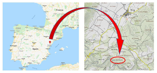
Figure 1.
Location map of Cova dels Cavalls rock art Site (Source: Institut Cartogràfic Valencià [35]).
2.2. Data Set Acquisition
The image set contains the so-called main hunting scene, which shows a group of hunters shooting arrows with their bows to a herd of deer (Figure 2). It is undoubtedly a vivid and spectacular human-centered scene, filled with movement, where the use of reddish pigment dominates [36].
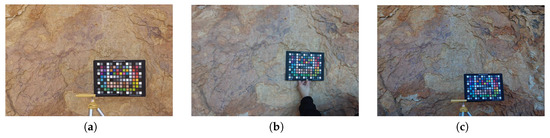
Figure 2.
Rock art images: (a) Fujifilm IS PRO (b) Sigma SD15 (c) Nikon D40.
Three different Single Lens Reflex (SLR) cameras were used in this study for image acquisition: a Fujifilm IS PRO with a Super CCD sensor (23 × 15.5 mm); a Sigma SD15 with a CMOS Foveon®X3 sensor (20.7 × 13.8 mm); and a Nikon D40, with a CCD sensor (23.7 × 15.6 mm). All those cameras allow taking pictures in a RAW format, which gives better results than processed images after characterization [20,21]. In fact, the use of RAW images allows us to disable the activation of the set of processing operations applied to the original images, such as white balancing, demosaicing or gamma correction, which implies the modification of the original data acquired by the sensor [20,37].
A main difference across cameras is their built-in image sensors. While the Super CCD sensor (Fujifilm IS PRO) and CCD sensor (Nikon D40) are monochrome with color filter array (CFA) and Bayern pattern for color interpolation, the Foveon®X3 sensor (Sigma SD15) is trichromatic, that is, it registers the color values for each channel separately without interpolation [38].
The scenes in the digital images should contain a chart as colorimetric reference. In our study we chose the X-rite ColorChecker®Digital SD chart, which is widely used in digital image processing pipelines. Although this color chart has 140 patches, we used only the 96 chromatic central chips (and 15 grey scale central ones) without considering the external patches on the edges. The RAW RGB data for these patches were extracted from the images using our own software named pyColourimetry [39].
The spectral reflectance data of the color patches from the ColorChecker were measured directly using the spectrophotometer Konica Minolta CM-600d. A total of 96 patches were measured under the CIE recommendations: 2° standard observer, and D65 illuminant. The spectral data collected can be easily transformed into CIE XYZ tristimulus values using well-known CIE formulae [40].
2.3. Colorimetric Camera Characterization Procedure
Image-based camera characterization is a well-known procedure described in numerous references [18,19,20,21,41]. The main stages of the imaged-based camera characterization procedure are (1) Training: sets the training data for model learning, (2) Regression model fitting and checking, and (3) Image characterization: creates the output sRGB image (Figure 3). In the following subsections, we provide detailed descriptions of each step.
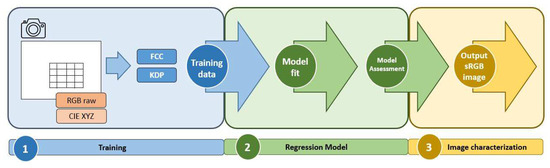
Figure 3.
Colorimetric camera characterization framework.
2.3.1. Training Data
Image-based characterization procedures rely on the training data set that typically permits model learning via the computation of the parameters of the selected mathematical function. The regression model is developed on the basis of the original data available: the camera responses (RAW RGB) and their colorimetric coordinates (CIE XYZ), both from the reference color chart.
As for the comparative analysis, we will separate two subsets of training data from each original dataset: the whole color patches (Full ColorChecker or FCC data set), and the selected dominant patches from the P-ASK framework (K-means dominant patches or KDP data set). Therefore, we will get two independent outcomes as outlined in Figure 3).
2.3.2. Regression Model and Accuracy Assessment
The image-based characterization procedure used in this study is based on an empirical regression model which defines the relationship between the input and output spaces. Different regression models have been used for camera characterization purposes, including polynomial models [41], artificial neural networks [42], polyharmonic splines [26] or Gaussian processes [25] to name a few. However, in recent years, research has focused on spectral recovery techniques [43]. In this paper, we used a classical second-order polynomial regression model, since it is computationally simple and gives valid results for archaeological applications [21,25].
In terms of good practice, the training data used for learning usually should not be used in model assessment since it may result in an overly optimistic prediction model error estimation. Instead, it is preferred to set aside an independent test data set used exclusively for model evaluation. Alternatively, a cross-validation framework may also be used, where the training data is repeatedly separated into training and testing sub data sets. In this study, a leave-one-out cross validation (LOOCV) procedure was performed for model accuracy assessment [44,45].
Two different metrics were used for the quality evaluation: the CIE XYZ residuals for model checking, and the color difference values in the colorimetric assessment of the characterized images. Regarding the color difference computation we used the formula [40] which performs well in rock art measurement conditions [25].
In colorimetric accuracy studies, it is usual to establish a threshold value known as “Just Noticeable Difference” (JND) or tolerance for . In this study, we set a JND value of four CIELAB units which ensures imperceptible variations to human vision [46].
2.3.3. Output sRGB Characterized Image
An additional transformation is required in order to reproduce the output CIE XYZ values on display or printing devices. We followed the International Electrotechnical Commission (IEC) specifications to transform the CIE XYZ tristimulus values into the sRGB color space, which is compatible with most digital devices [47].
2.4. K-means Clustering Technique
K-means is a center-based clustering algorithm widely used in different applications of data mining, machine learning and pattern recognition [48]. K-means aims to minimize the mean squared distance from each N-data point to its K-nearest cluster center, following four basic steps to: (1) set initial K cluster centers, (2) group samples in the K clusters, (3) recompute the new K cluster centers, (4) iterate the process until the algorithm converges [49,50,51].
Since the introduction of the K-means algorithm in its current form [48], different alternatives and improvements to achieve better performance have been published, including an algorithm less sensitive to initialization settings [50] or filtering algorithms [52].
In this study, we developed a Python script to apply the K-means algorithm to our specific problem, which is to select dominant colors in camera characterization. The Python script leverages the Scikit-learn package (v0.21.3) [53] which includes an optimized implementation of the K-means algorithm together with others machine learning algorithms for supervised and unsupervised classification applications [53,54]. Particularly, we used the KMeans function (see [55] for more details).
However, before applying the K-means clustering algorithm, it is required to take into account some quirks associated with this technique. K-means yields accurate results when the K number of clusters and its initial centroid points are properly defined. Moreover, as an iterative technique, the K-means algorithm is potentially sensitive to initial starting conditions [56]. Thus, an inappropriate determination of initial parameters could highly decrease the accuracy of the results [57].
In our study, the inappropriate selection of clusters means that the results will not match with the real dominant colors present in the image. Therefore, it is necessary to overcome the negative effects derived from K-means initial approximations by properly setting the K number of clusters for optimal implementation of the algorithm and proper determination of the initial values.
2.4.1. Optimal K Number of Clusters
The first issue to address is how to set the optimal K number of clusters and their corresponding initial centroids, since the K clusters should be known beforehand and specified by the user. Several factors could affect the selection of K such as the level of detail, the internal distribution of the samples values or its interdependence with other objects [49,58]. Different methods can be applied for selecting the number of clusters, such as those based on automatic process [57], probabilistic clustering approaches or visual verification [58].
To determine an appropriate number of clusters for K-means clustering, a trial-and-error process experiment was conducted. We used the rock art scene images as input data to evaluate the processing time for different values of K. In general, K-means clustering is used not only to determine the natural groups in the data, but also to identify irregularities in their distribution. However, in rock art scenes the data tends to be uniform, and we expect a set of dominant colors made of a reduced number of instances, which in turn will be highly correlated. In order to determine a proper value of K, we assessed the processing time for values of K in the range 10–100.
2.4.2. Clustering Algorithm
The basic K-means algorithm [48] has been updated to improve its effectiveness, robustness and convergence speed [50]. Some of the most widely known implementations are: Forgi [59], expectation-maximization or EM-Style algorithm [60,61], Standard algorithm (LLoyd’s algorithm or Voroni iteration) [62], and Elkan [63].
Two of those algorithms are implemented in the Scikit-learn KMeans function: EM-style for sparse data and Elkan for dense data. Users can specify their choice via the “algorithm” parameter, using “full” or “elkan” for the EM-style or Elkan option respectively (see an example of code in Section 2.5.1 for syntax details). Given that our study is based on moderately large data sets from the RGB triplets of the digital image, the optimal algorithm to compute K-means is Elkan. The Elkan algorithm is an optimized version of the standard K-means clustering method based on the triangle inequality. The aim is to reduce its processing time by avoiding unnecessary distance calculations [63].
2.4.3. Initial Starting Conditions
The K-means algorithm searches for the optimal data partition into the K clusters established by the user. Thus, K-means provides a set of K point clusters defined by their centroids, and assigns every data point into its nearest cluster centroid. However, the final group partition is highly dependent on the initial cluster centers. Since the centroids of the clusters are usually unknown in advance, the K-means algorithm relies on a random process to set the starting cluster centroids, which are frequently chosen uniformly on the range of the data [56].
The random initialization method takes a set of K arbitrary centers uniformly selected at random as starting points. The drawback of pure random selection is the high number of iterations required to converge, and furthermore different runs with the same data do not give exactly the same results. In order to overcome this limitation, the K-means++ initial method was developed to improve algorithm speed and give more consistent results despite being a random method [64]. In fact, this is the default option for the KMeans function.
The lack of consistency of random methods has been the subject of previous research. However, initialization methods based on randomness are considered as a proper selection procedure that gives satisfactory results [49]. In this study we run a simple experiment to find out the optimal initial values based on random algorithms. We just run the algorithm several times which has been reported as a suitable method to account for randomness issues [56]. We used the Scikit-learn K-means++ initial method, since it is a optimized and fast random process [64]. This analysis will allow us to determine whether or not the algorithm consistently provides the same dominant color patches although being based on a random process.
2.5. Color Patch Adaptive Selection with K-Means (P-ASK)
The aim of the P-ASK procedure is to establish a methodology for the automatic selection of color training samples for camera characterization, and keep the process as simple as possible. The P-ASK framework can be separated into two main stages: the application of the K-means algorithm for the dominant color extraction of the input image, and the identification of dominant color patches as training data for the camera characterization. The first stage of this procedure can be considered as an specific image segmentation application, since it is intended to group the pixels of an image according to their color similarity.
The main steps in P-ASK framework (Figure 4) are: (1) create a white balanced image (D65 illuminant), (2) select support and pigment samples, (3) extract K-means dominant colors, and (4) identify dominant color patches. Further detailed explanations about those steps are given in the subsections below.
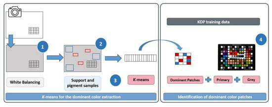
Figure 4.
P-ASK framework.
2.5.1. K-means Dominant Color Extraction
The first aim of P-ASK is the dominant color extraction from a digital image. Previously to applying the K-means clustering algorithm two basic operations are required: white balance and sample selection.
The CIE XYZ data were acquired under the D65 illuminant specification. Thus, in order to find the patches corresponding to the dominant colors, the RGB values should be strictly registered under the D65 illuminant. Since usually it is not possible to work under controlled illuminant conditions in open-air cultural heritage sites such as rock art archaeological shelters, we used a white balanced image under the hypothesis of D65 illuminant as an approximation to natural daylight. From an original RAW image, it is possible to obtain a white balanced image using the rawpy Python package [65].
One problem associated with the application of the K-means clustering algorithm to full images is the significant increase of the convergence time, given the large size of the data set. A simple and suitable option for our framework is to reduce the image size to compute only a selected image samples instead of full images. For rock art applications, the main interest is focused on defining the representative colors, especially of the pigments an the main support colors. Thus, we selected a set of samples from significant support and pigment areas for the K-means computation (Figure 5).
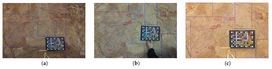
Figure 5.
Support and pigment samples: (a) Nikon D40 image (b) Sigma SD15 image (c) Fujifilm IS PRO image.
Finally, the digital data are passed into the algorithm as RGB triplets (nRGBdarray) for subsequent computing. The Python code line which runs the K-means algorithm is as follows:
where the main parameters introduced to the algorithm are: the K number of clusters; Elkan as the algorithm since it works well for dense data; and the K-means++ initialization method. The remaining parameters have been assigned to the default values of the Scikit-learn KMeans function [55].
| clt = KMeans(n_clusters = K, init = "K-means++", n_init = 10, max_iter = 300, |
| tol = 0.0001, precompute_distances= "auto", verbose=0, |
| random_state = None, copy_x = True, n_jobs = None, |
| algorithm = "elkan").fit(nRGBdarray)} |
2.5.2. Identification of Dominant Color Patches
The outcome of the K-means algorithm consists of a set of centroids, one for each K cluster. Those coordinates are a list of K RGB triplets of dominant colors, which represent the main colors found in the input digital image. The second stage seeks the correct identification of the color chart patches from the dominant colors from the K-means algorithm.
The dominant colors extracted in the RGB color space can be easily transformed to CIE XYZ tristimulus values [40] and CIELAB coordinates [66] as required for subsequent processing. With the CIELAB coordinates the color differences are computed between each dominant color and the whole set of color chips. It is then possible to identify the nearest patches to each dominant color found in the image by looking for the lowest .
For the identification of color patches, four different approaches are tested after varying the input data and colorimetric criteria: (1) using the n nearest patches found in the whole image (NN), (2) removing the color chart from the scene and identifying the n nearest patches (RC), (3) using a set of samples corresponding to pigment and support classes and creating a new, joined synthetic image (JS), and (4) using the same sample set used in (3), but computing each class separately (SS). Note that while in the first method we do not specify any colorimetric criteria, in the remaining cases we search for the nearest patches to each dominant color with color differences less than 10 CIELAB units (maximum value allowed in cultural heritage guidelines [46]).
Although the use of the nearest patches extracted from dominant colors using K-means offer accurate colorimetric results, it does not always imply a proper output characterized image, that is, an image with true colorimetric sense. Our experience shows that a set of minimum fixed patches should be included in order to obtain accurate and colorimetrically sound characterized images [24], including the primary additive colors [E4, F4, G4] and the basic grayscale chips [E5, F5, G5, H5, I5, J5] (highlighted in Figure 4, step number 4).
3. Results
In this Section we describe all processing tasks, together with their output results, that support some practical considerations to define the P-ASK. Specific tests were run to define the optimal parameters of the algorithm and to assess its performance in controlled laboratory conditions as well as in rock art sites with uncontrolled light conditions.
3.1. Setting the Optimal Parameters for the K-Means Clustering Algorithm
As reported in Section 2.4, several factors could affect the results of the K-means clustering method, namely the K number of clusters and centroids to generate, the input size image, the initialization method and the algorithm applied.
3.1.1. K Number of Clusters
The first issue to consider is the proper determination of the K number of clusters. That number can be determined by simple heuristics, for instance by testing several values of K and taking some convenient value, or with specific data mining tools such as the Elbow [67,68] or the Silhouette graphic methods [69].
A preliminary experiment was conducted under the worst-case scenario; that is, using the whole image as input data which gives some sort of upper bound in terms of computation time. The results about the running time required for computing K-means clustering are displayed in Table 1. According to those results, K = 24 seems to be an acceptable number of clusters. The choice of this value, however, is based on the running time experiment only, and thereby it is somewhat arbitrary. It is timely, then, to confirm our choice by other means, with a consensus across numerical results, graphical tools and colorimetric criteria.

Table 1.
Evaluation of K-means running time with different values of K.
From a color viewpoint, our study aims at characterizing digital cameras properly with a reduced number of color chips whether it is possible, which is in many ways is rather the same as performing color quantization of the image. In addition, our application field, the recording of Levantine rock art archaeological shelters requires a very specific color domain, mostly in the chromatic range of red, brown, and yellow colors which in turn are little saturated (check dominant colors extracted in rock art images in Section 3.3). Thus, a number of 24 seems a reasonable choice, provided that output images are rigorous duplicates of the real specimens (Section 3.4 and Section 3.5 report on this point).
In addition to colorimetric criteria, we tested the Elbow and Silhouette methods which provide graphic aid to determine the right K number in clustering problems. The Elbow method [67,68] consists of running the K-means algorithm on the dataset for a range of values of K, and calculate the distortion and inertia values for each K. The distortion value is the average of the Euclidean distance between all the cluster centroids for each K; the inertia is calculated as the sum of the Euclidean distances to their nearest cluster centroids. Those parameters are useful to describe how close the different K clusters are to each other. Clusters that are too close may be an indication of incorrect data partitioning, so that they could be integrated into the same cluster.
Figure 6 shows the plot of the Elbow analysis using the inertia criterion, which exhibits a sharp change in slope around K = 24 (cf. vertical red line on Figure 6) and linear behavior beyond this K value. This result is compatible with the previous running time test (Table 1).
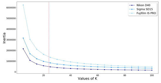
Figure 6.
Elbow method using inertia.
The silhouette analysis is another useful tool to analyze the separation distance among cluster centroids, which ultimately reports on the quality of the data partition. In this method, each K cluster is represented by its so-called silhouette, which is calculated as a result of the comparison between its tightness and separation [69]. The mean silhouette width, also known as silhouette coefficient or silhouette score, provides an evaluation of clustering validity, with a value within the range [−1,1]. Negative values indicate wrong cluster assignment, whereas positive values (the closer to 1, the better) indicate well-separated neighboring clusters.
We run the Silhouette analysis using the Scikit-learn module which implements the method in two functions called metrics.silhouette_score and metrics.silhouette_samples. Both functions require the output of the KMeans function as input parameter [70]. Figure 7 displays the graphic results given by the Silhouette method for the Fujifim IS PRO image with K = 24. All silhouette coefficients are similar (around 0.6) with narrow fluctuations, which is an indicator of good clustering for the chosen number of clusters K [71]. Furthermore, all coefficients are above the average silhouette score (vertical red dashed line in Figure 7) which confirms the value 24 as a proper choice for clustering. The silhouette method also provides a graph for visualizing the clustered data (Figure 7b), which shows a very dense, but well separated, data set as expected in our case study.
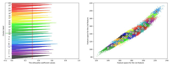
Figure 7.
Silhouette analysis for the Fujifilm IS PRO.
3.1.2. K-means Initialization
Once the K number of clusters is determined, the next step is the proper selection of the algorithm and the initialization method to run K-means. The KMeans function in the Scikit-learn Python package provides two algorithms: EM-style and Elkan. Since we usually work with large, dense data sets collected from digital images, we chose the Elkan algorithm which is known to perform well in such circumstances [55,63].
The second parameter to be determined is the initialization method of the algorithm. As usual in all implementations, the KMeans function relies on a pseudorandom parameter to start the process. Theoretically, the best option in the KMeans function is the K-means++ method, which is an optimized and fast, but still random approach [55]. A random initialization is a convenient approach to create self-starting methods and reduce user intervention. However, it has the potential drawback of returning different or inconsistent results in different runs [57,58]. This characteristic is clearly against common scientific and engineering conventions such as repeatability or reproducibility, and its effects on the results must be verified.
In our study, the K-means algorithm was run multiple times (100 realizations) to find out whether or not the K-means reported the same set of dominant colors in a consistent manner. We then grouped the results by dominant color and created a list of RGB triplets for each dominant color found. Every list was processed to compute basic statistics: mean, minimum, maximum, standard deviation, coefficient of variation, and so on. Those results confirmed that the K-means algorithm reports dominant colors very consistently. The RGB differences within every dominant color were all negligible which also applies when we computed the differences of the data (Figure 8). All color difference values were less than 1 CIELAB unit ( < 1, red line on Figure 8a), clearly under the JND threshold value. The standard deviation error was less than three digital level units (Figure 8b). Furthermore, and most importantly, the set of colors is consistently in the same range, which confirms the suitability of the K-means algorithm to determine dominant color in rock art scenes for camera characterization purposes.
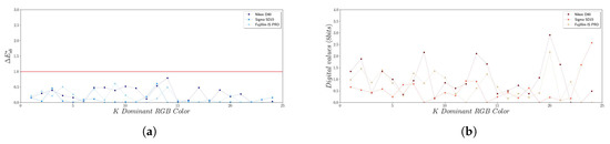
Figure 8.
Randomness assessment: (a) color differences (b) Standard deviation error.
3.1.3. Identification of Dominant Color Patches
The input image size, that is the data set size, has a direct effect on the processing time required for the K-means algorithm (Section 3.1.1). A simple solution to reduce the processing time is to use small sample images instead of the complete picture. However, our study seeks an efficient methodology not only in terms of computation speed, but mostly regarding its performance in identifying color patches. In this line, four different methods were tested prior to setting the optimal path for identifying color patches. Table 2 shows the results of each method. Those four methods are briefly described as follows:
Table 2.
Comparison of four methods to identify dominant color patches.
- Nearest n-patches (NN). The complete image is processed.
- Remove ColorChart (RC). The color chart is removed from the original image.
- Joined samples (JS). Pigment and support samples are merged in a new synthetic data set and processed together.
- Split samples (SS). Pigment and support samples are processed using two different data sets.
The NN method detected the highest number of patches using the four nearest patches (n = 4). It should be noted, though, that there are no colorimetric restrictions in this approach, which means that some patches can be out of the range of dominant colors extracted from the images or, in other words, some patches may not fit the real rock art scene. This point came out when observing some visual inconsistencies between the patches detected by the algorithm and the scenes under study. The other methods detected less patches but returned better colorimetric results. This was the expected result since colorimetric constraints somehow guarantee better fit of the selected patches to the scene. The RC method systematically gave the smallest number of patches and should be rejected since the other three methods provide similar results regardless of the camera sensor in use. The method that offered the best results was the SS, therefore, splitting samples for the pigment and the support areas seems to be the most reasonable choice.
We also conducted a detailed analysis of the SS method with focus on performance as a function of the number of clusters K (Table 3 and Figure 9). According to these results, the number of color patches detected stabilizes, whereas the processing time grows linearly without improving the collection of color patches. Therefore, based on these results, the best option seems to be the SS method with K = 24.
Table 3.
Assessment of the SS method for the identification of dominant patches.
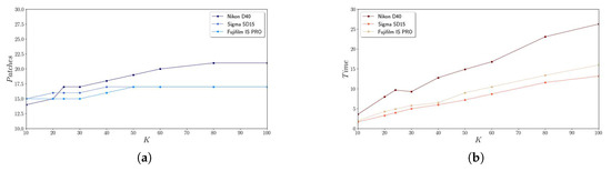
Figure 9.
Graphic results for the SS method: (a) Patches identified; (b) Processing time.
3.2. Test on the DigiEye Imaging System
Before applying the P-ASK framework on rock art images, several tests were run in a laboratory environment under highly controlled light conditions. We used the DigiEye imaging system [72] which allows taking pictures in an optimal environment to conduct colorimetry experiments. The images were captured with the SLR Nikon D40 camera and the color reference was the X-rite Passport color chart under the D65 illuminant (Figure 10).
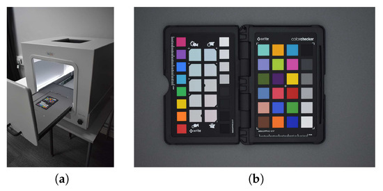
Figure 10.
DigiEye imaging system: (a) DigiEye system (without camera integrated) (b) Nikon D40 test image (D65 illuminant).
The test presented in this Section is a reduced version of the whole P-ASK method. In the test we obtained images of the color checker, without rock art specimens, which provides some sort of “benchmark environment” to assess the quality of P-ASK (Figure 11).
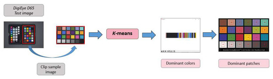
Figure 11.
P-ASK framework adapted to the DigiEye D65 image acquired with the Nikon D40.
The input image was a clipped picture of the X-rite color checker and the working parameters were: K = 25 (24 colored patches and one color for the background), Elkan algorithm, K-means++ initialization, and the SS method for the identification of the dominant patches. Figure 11 shows the performance in the identification of colors on the chart. Our method can perfectly identify all colors present in the chart without any missing patches. This result is certainly compelling and shows the potential of P-ASK to adapt to the whole chromatic domain of the scene, which makes the method a suitable choice to be applied in documenting rock art images.
3.3. Assessment of the P-ASK Framework on Rock Art Images
Since the P-ASK framework provides good results in laboratory conditions, the next step is the assessment using images collected in rock art shelters. In order to simplify this paper, we present the results for the Fujifilm IS PRO image only. We should note that all steps described in Figure 4 are carefully computed, using the parameters established in previous sections: K = 24, Elkan algorithm, K-means++ initialization, and SS method. We emphasize once again that the aim of the P-ASK framework is to (a) extract the dominant colors present on the rock art scene, (b) identify its corresponding patches in the color chart, and (c) carry out the characterization using those patches as training data.
From the Fujifilm IS PRO white-balanced image, a set of twelve samples were collected for the extraction of dominant colors, five samples for the support (S1, S2, S3, S4 and S5), and seven for the pigment (P1, P2, P3, P4, P5, P6 and P7). Figure 5c shows the sampling areas that were clipped to get the samples for subsequent processing. Figure 12 contains a detailed description of pigment sample P1 consisting of the detail clipped image, the color palette of the dominant colors, and its frequency histogram. P-ASK provides this information for each sample separately.
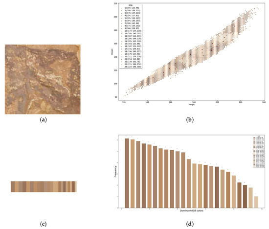
Figure 12.
Graphic description of the pigment sample (P1): (a) clipped detail image, (b) K-means centroids, (c) Dominant color palette, (d) Dominant color frequency histogram.
The last step prior to camera characterization is to select a list of patches from the color chart that match with the dominant colors obtained from the samples. The results provided by P-ASK consist of 9 patches for the support and 14 for the pigment (see a summary in Table 4 and Figure 13). This is the expected result considering that the support rock material is highly uniform and requires less colors to be characterized. Note also that duplicates appear across samples of the same class (either pigment or support) as well as across samples of different classes. This characteristic is also expected since the sampling areas for pigment characterization also contain some amount of support.
Table 4.
Color Patches detected from the Fujifilm IS PRO samples.
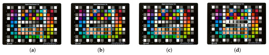
Figure 13.
Color patches detected: (a) Support samples; (b) Pigment samples; (c) Support-pigment; (d) KDP training samples.
A total of 15 color patches are identified from the chromatic image information with P-ASK (Table 4 and Figure 13c). We have to note that none of the previous methods integrate “color insight” in their rationales. It is the user’s responsibility to append such insight, as we did when extending the set of color chips with three primaries and six grays. Thus, the KDP training dataset for the Fujifilm IS PRO camera consists of a total of 24 color patches (cf. Figure 13d).
3.4. Model Accuracy Assessment of the Image-based Characterization
Two different sets of training data are used to build the regression model used in the camera characterization procedure: the FCC set (96 samples) and the KDP (24 selected reported by P-ASK). We conducted a comparison between the results achieved for both training data sets. Table 5 shows the basic statistics of the LOOCV residuals of the CIE XYZ predicted values after model adjustment. For the sake of completeness, we also include the residuals of the FCC model applied to the dominant patches in the KDP model, which helps in comparing all data sets. The histograms of the LOOCV CIE XYZ residuals are also displayed in Figure 14.
Table 5.
CIE XYZ Residuals of the FCC and KDP models.
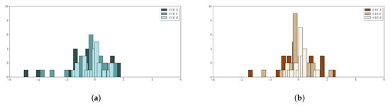
Figure 14.
LOOCV CIE XYZ Residuals histogram: (a) FCC (24 patches) (b) KDP (24 patches).
By comparing the residuals of the FCC (with 24 patches) and the KDP model, we find slightly better results in the KDP model, especially in the minimum and the standard deviation statistics (Table 5, Figure 14a,b).
Although the assessment of residuals is very useful to evaluate the predictive capability of the regression model, the computation of the color differences is required in colorimetry experiments to rigorously analyze the accuracy achieved after camera characterization. Table 6 shows basic color difference statistics computed for the FCC and KDP models. Once again, the values obtained by the KDP model show an improvement in terms of colorimetric accuracy when compared with the FCC model. The better results given by the KDP model can be seen graphically in the one-to-one color patches plot displayed in Figure 15. All in the KDP samples were lower than in the FCC samples, and always under the JND threshold value fixed in 4 CIELAB units (cf. Figure 15a,b).
Table 6.
color differences in the FCC and KDP characterization experiments.
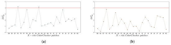
Figure 15.
color differences: (a) FCC (24 patches); (b) KDP (24 patches).
3.5. Output sRGB Characterized Images
Ideally, the final outcome obtained through the characterization process is an image with “colorimetric characteristics.” A common approach to preserve such characteristics in digital pictures is the use of the sRGB space, where the RGB data are defined in a physically based, device-independent color space via transformation functions of CIE XYZ tristimulus values [47]. The output sRGB characterized images are shown in Figure 16. By observing those sRGB images, it is evident that the results are very satisfying in visual terms, regardless of the training data used for the regression model.
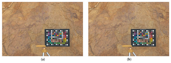
Figure 16.
Output sRGB characterized images: (a) FCC training data (96 patches) (b) KDP training data (24 patches).
Although the comparison between the two models confirms that the KDP model performs better in numerical terms, the images provided by the two different training datasets show that both characterization approaches transform successfully RGB data to the CIE XYZ independent color space. It is challenging, even for experienced observers, to perceive any visual differences between the two output images (cf. Figure 16a,b).
In addition to the numerical computations, we created a mapping image with the color differences between the characterized images obtained with the FCC and the KDP training data sets (Figure 17). The predominant green color present on the difference mapping image indicates that the values of color difference values are less than 2 CIELAB units (see map key in Figure 17), which is a very good result in colorimetric terms. Actually, we found higher differences in two cases corresponding to (a) cracks in the rock, where hard shadows are produced (yellow pixels with differences between 2 and 3 units), and (b) some patches of the color chart out of the color domain of the scene (differences greater than 2 units coded with yellow, orange and red pixels). Since the focus of the study is on accurate colorimetric analysis of the pigmented areas of the rock art scenes, we can confirm that the P-ASK framework proposed in this study provides very satisfactory results for the camera characterization.
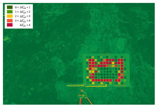
Figure 17.
mapping image (96-24 patches).
4. Discussion
The generic aim of clustering applications is the natural grouping of specimens that share similar properties within a data set. In this study, we established the P-ASK framework which leverages the K-means technique for automatic training in the selection of a simplified set of color patches, and properly capture the dominant color characteristics of rock art scenes.
Since the K-means algorithm is sensitive to the initial approximations given by the user [56,57], a set of preliminary experiments were conducted to set proper values for the number of clusters, the working algorithm and the initialization method. According to our results, the suggested parameters to run K-means were appropriate, and the algorithm implemented in the KMeans function of the Scikit-learn module proved to be a valid option for clustering operations as well.
However, the K-means algorithm is slow for large data sets, particularly those based on digital images. In our paper, we suggest an alternative approach to extract the dominant colors which consists of using a reduced number of image samples clipped from the full image. By using image sampling, the running time was considerably reduced. For instance, run time decreased from 18.2 min to 4.9 min when using the Fujifilm IS PRO image for K = 24 clusters (cf. Table 3 with Table 1 in Section 3).
The experiment conducted to identify the effect of randomness on the K-means clustering technique showed that the dominant color set returned from multiple runs was highly consistent [48]. In this regard, Figure 8 shows color differences less than 1 CIELAB unit for the dominant colors obtained in 100 realizations, with similar negligible results in units of pixel RGB digital values.
Moreover, the capability of P-ASK to identify the dominant colors into the ColorChecker offers very good results (see Table 4 and Figure 13), and allowed extracting a set of color chips from the chart to create a reduced training data set for camera characterization in a simple and fast way. By using this framework, we proved that the characterization approach based on the KDP training data gives accurate results which parallel those obtained in common practice, that is, using the whole set of color chips for model learning.
Although previous studies recommend the use of large training data sets for camera characterization [22,41,73,74], the results obtained with the P-ASK framework show that it is possible to use a reduced number of training samples without loss of accuracy in colorimetric terms. It is worth noting that the CIE XYZ residuals (Table 5) and the color differences (Table 6) obtained using the KPD data set are in fact slightly better. In view of the outcome images, it is evident that sRGB characterized images were satisfactorily obtained (Figure 16), which is confirmed by the color difference map image where differences under 2 CIELAB units prevail over the whole image, particularly in the area of interest for archaeological applications (Figure 17).
As an aside, we would like to note that the specific imaging hardware, i.e., the digital camera used for graphical documentation, is a key point that must be considered prior to characterization. We know from previous research that built-in imaging sensors have a considerable impact on the final outcome. In this sense, we presented the results of the Fujifilm IS PRO camera which is known to work very well, not only in the characterization procedure [25], but also in terms of image noise [75].
5. Conclusions
In this paper, we propose a new P-ASK framework for consistent and accurate archaeological color documentation. The graphic and numeric results obtained after the characterization of rock art images are highly encouraging and confirms that P-ASK is a suitable technique to use in the context of the image-based camera characterization procedure. Our characterization approach based on a reduced set of dominant colors offers several advantages. On the one hand, it implies the reduction of the training set size, and thereby, the computing time required for model training is less than in the regular approach with all color chips. On the other hand, there is an improvement derived from the use of a reduced number of specific color patches, which adjust better to the chromatic range of the scene, and yields better results in the output characterized images. We consider this point as a major contribution in this paper.
The tests conducted in our study confirmed that P-ASK is robust to random issues in the K-means stage and works very well with a specific sampling of the elements of interest in the rock art scene. This point leads us to envision future research lines focused on developing specific color charts for archaeological applications, and even for specific cultural heritage objects, monuments and sites. In summary, the results achieved in this study show that P-ASK is a suitable tool for the proper and rigorous use of color camera characterization in archaeological documentation, and can be integrated into the regular documentation workflow with minimum effort and resources.
Author Contributions
Conceptualization, A.M.-T.; Formal analysis, A.M.-T.; Funding acquisition, J.L.L.; Methodology, A.M.-T.; Software, A.M.-T. and Á.M.-M.; Supervision, Á.M.-M., J.L.L. and S.W.; Writing—original draft, A.M.-T.; Writing—review & editing, Á.M.-M., J.L.L. and S.W. All authors have read and agreed to the published version of the manuscript.
Funding
This research is partly funded by the Research and Development Aid Program PAID-01-16 of the Universitat Politècnica de València, through FPI-UPV-2016 Sub 1 grant.
Acknowledgments
The authors would like to thank the Direcció General de Cultura i Patrimoni, Conselleria d’Educació, Insvestigació, Cultura i Esport de la Generalitat Valenciana, their authorization to carry out the 3D documentation in the Cova dels Cavalls site in Tírig (Castelló, Spain). The authors are also very grateful for the support of the staff at Colour Research Group from the University of Leeds (UK), who kindly allowed the use of their facilities and colorimetric instrumental during a research fellowship of the corresponding author.
Conflicts of Interest
The authors declare no conflict of interest. The funders had no role in the design of the study; in the collection, analyses, or interpretation of data; in the writing of the manuscript, or in the decision to publish the results.
Abbreviations
The following abbreviations are used in this manuscript:
| CIE | Commission Internationale de l’Éclairage |
| FCC | Full ColorChecker data set |
| IEC | International Electrotechnical Commission |
| JND | Just noticeable difference |
| JS | Joined samples |
| KDP | K-means dominant patches data set |
| LOOCV | Leave-one-out cross-validation |
| NN | Nearest n-patches |
| P-ASK | Patch Adaptive Selection with K-means |
| RC | Remove ColorChart |
| RMS | Root-mean-square |
| SLR | Single Lens Reflex |
| SS | Separated samples |
References
- Sesana, E.; Gagnon, A.S.; Bertolin, C.; Hughes, J. Adapting cultural heritage to climate change risks: Perspectives of cultural heritage experts in Europe. Swiss J. Geosci. 2018, 8, 305. [Google Scholar] [CrossRef]
- Cerra, D.; Plank, S.; Lysandrou, V.; Tian, J. Cultural Heritage Sites in Danger—Towards Automatic Damage Detection from Space. Remote Sens. 2016, 8, 781. [Google Scholar] [CrossRef]
- Barrile, V.; Fotia, A.; Bilotta, G.; De Carlo, D. Integration of geomatics methodologies and creation of a cultural heritage app using augmented reality. Virtual Archaeol. Rev. 2019, 10, 40–51. [Google Scholar] [CrossRef]
- Lerma, J.L.; Navarro, S.; Cabrelles, M.; Villaverde, V. Terrestrial laser scanning and close range photogrammetry for 3D archaeological documentation: the Upper Palaeolithic Cave of Parpalló as a case study. J. Archaeol. Sci. 2010, 37, 499–507. [Google Scholar] [CrossRef]
- Previtali, M.; Valente, R. Archaeological documentation and data sharing: digital surveying and open data approach applied to archaeological fieldworks. Virtual Archaeol. Rev. 2019, 10, 17–27. [Google Scholar] [CrossRef]
- Pan, Y.; Dong, Y.; Wang, D.; Chen, A.; Ye, Z. Three-dimensional reconstruction of structural surface model of heritage bridges using UAV-based photogrammetric point clouds. Remote Sens. 2019, 10, 1204. [Google Scholar] [CrossRef]
- Tang, P.; Chen, F.; Zhu, X.; Zhou, W. Monitoring cultural heritage sites with advanced multi-temporal InSAR technique: The case study of the Summer Palace. Remote Sens. 2016, 8, 432. [Google Scholar] [CrossRef]
- Padín, J.; Martín, A.; Anquela, A.B. Archaeological microgravimetric prospection inside don church (Valencia, Spain). J. Archaeol. Sci. 2012, 39, 547–554. [Google Scholar] [CrossRef][Green Version]
- Rogerio-Candelera, M.A. Digital image analysis based study, recording, and protection of painted rock art. Some Iberian experiences. Digit. Appl. Archaeol. Cult. Herit. 2015, 2, 68–78. [Google Scholar] [CrossRef]
- Federica, M.; Di Giulio, R.; Piaia, E.; Medici, M.; Ferrari, F. Enhancing Heritage fruition through 3D semantic modelling and digital tools: the INCEPTION project. IOP Conf. Ser. Mater. Sci. Eng. 2018, 364, 012089. [Google Scholar]
- Cabrelles, M.; Blanco-Pons, S.; Carrión-Ruiz, B.; Lerma, J.L. From Multispectral 3D Recording and Documentation to Development of Mobile Apps for Dissemination of Cultural Heritage. In Cyber-Archaeology and Grand Narratives: Digital Technology and Deep-Time Perspectives on Culture Change in the Middle East; Levy, T.E., Jones, I.W.N., Eds.; Springer: Cham, Switzerland, 2018; pp. 67–90. [Google Scholar]
- Ippoliti, E.; Calvano, M. Enhancing the Cultural Heritage Between Visual Technologies and Virtual Restoration. In Digital Curation: Breakthroughs in Research and Practice; IGI Global: Hershey, PA, USA, 2019; pp. 309–348. [Google Scholar]
- del Hoyo-Meléndez, J.M.; Carrión-Ruiz, B.; Riutort-Mayol, G.; Lerma, J.L. Lightfastness assessment of Levantine rock art by means of microfading spectrometry. Color Res. Appl. 2019, 44, 547–555. [Google Scholar] [CrossRef]
- Korytkowski, P.; OlejniK-Krugly, A. Precise capture of colors in cultural heritage digitization. Color Res. Appl. 2017, 42, 333–336. [Google Scholar] [CrossRef]
- Boochs, F.; Bentkowska-Kafel, A.; Degrigny, C.; Karaszewski, M.; Karmacharya, A.; Kato, Z.; Picollo, M.; Sitnik, R.; Trémeau, A.; Tsiafaki, D. Colour and Space in Cultural Heritage: Key Questions in 3D Optical Documentation of Material Culture for Conservation, Study and Preservation. In Lecture Notes in Computer Science, Proceedings of the Digital Heritage. Progress in Cultural Heritage: Documentation, Preservation, and Protection. EuroMed 2014, Limassol, Cyprus, 3–8 November 2014; Springer: Berlin, Germany, 2014; Volume 8740, pp. 11–24. [Google Scholar]
- Molada-Tebar, A.; Marqués-Mateu, Á.; Lerma, J.L. Correct use of color for cultural heritage documentation. ISPRS Ann. Photogramm. Remote Sens. Spatial Inf. Sci. 2019, IV-2/W6, 107–113. [Google Scholar] [CrossRef]
- Sharma, G. Color fundamentals for digital imaging. In Digital Color Imaging Handbook; CRC Press: Boca Raton, FL, USA, 2003; p. 94. [Google Scholar]
- Martinez-Verdu, F.; Pujol, J.; Capilla, P. Characterization of a digital camera as an absolute tristimulus colorimeter. J. Imaging Sci. Technol. 2003, 47, 279–295. [Google Scholar]
- Bianco, S.; Schettini, R.; Vanneschi, L. Empirical modeling for colorimetric characterization of digital cameras. In Proceedings of the 2009 16th IEEE International Conference on Image Processing (ICIP), Cairo, Egypt, 7–10 November 2009; Volume 1, pp. 3469–3472. [Google Scholar]
- Westland, S.; Ripamonti, C.; Cheung, V. Characterisation of Cameras. In Computational Colour Science Using MATLAB®, 2nd ed.; John Wiley & Sons, Inc.: Chichester, UK, 2012; pp. 143–157. [Google Scholar]
- Molada-Tebar, A.; Lerma, J.L.; Marqués-Mateu, Á. Camera characterization for improving color archaeological documentation. Color Res. Appl. 2018, 43, 47–57. [Google Scholar] [CrossRef]
- Chou, Y.; Luo, M.R.; Li, C.; Cheung, V.; Lee, S. Methods for designing characterisation targets for digital cameras. Color. Technol. 2013, 129, 203–213. [Google Scholar] [CrossRef]
- Zhang, X.; Wang, Q.; Li, J.; Zhou, X.; Yang, Y.; Xu, H. Estimating spectral reflectance from camera responses based on CIE XYZ tristimulus values under multi-illuminants. Color Res. Appl. 2017, 42, 68–77. [Google Scholar] [CrossRef]
- Molada-Tebar, A.; Marqués-Mateu, Á.; Lerma, J.L. Camera Characterisation Based on Skin-Tone Colours for Rock Art Recording. Proceedings 2019, 19, 12. [Google Scholar] [CrossRef]
- Molada-Tebar, A.; Riutort-Mayol, G.; Marqués-Mateu, Á.; Lerma, J.L. A Gaussian Process Model for Color Camera Characterization: Assessment in Outdoor Levantine Rock Art Scenes. Sensors 2019, 19, 4610. [Google Scholar] [CrossRef]
- Colantoni, P.; Thomas, J.B.; Hardeberg, J.Y. High-end colorimetric display characterization using an adaptive training set. J. Soc. Inf. Disp. 2011, 19, 520–530. [Google Scholar] [CrossRef]
- Cheung, V.; Westland, S. Methods for Optimal Color Selection. J. Imaging Sci. Technol. 2006, 50, 481–488. [Google Scholar] [CrossRef]
- Eckhard, T.; Valero, E.M.; Hernández-Andrés, J.; Schnitzlein, M. Adaptive global training set selection for spectral estimation of printed inks using reflectance modeling. Appl. Opt. 2014, 53, 709–719. [Google Scholar] [CrossRef] [PubMed]
- Liu, Z.; Liu, Q.; Gao, G.; Li, C. Optimized spectral reconstruction based on adaptive training set selection. Opt. Express 2017, 25, 12435–12445. [Google Scholar] [CrossRef]
- Shen, H.L.; Zhang, H.G.; Xin, J.H.; Shao, S.J. Optimal selection of representative colors for spectral reflectance reconstruction in a multispectral imaging system. Appl. Opt. 2008, 47, 2494–2502. [Google Scholar] [CrossRef] [PubMed]
- OlejniK-Krugly, A.; Korytkowski, P. Precise color capture using custom color targets. Color Res. Appl. 2020, 45, 40–48. [Google Scholar] [CrossRef]
- Mohammadi, M.; Nezamabadi, M.; Berns, R.S.; Taplin, L.A. Spectral Imaging Target Development Based on Hierarchical Cluster Analysis. Color and Imaging Conf. 2004, 1, 59–64. [Google Scholar]
- Xu, P.; Xu, H.; Diao, C.; Ye, Z. Self-training-based spectral image reconstruction for art paintings with multispectral imaging. Appl. Opt. 2017, 56, 8461–8470. [Google Scholar] [CrossRef]
- UNESCO. Rock Art of the Mediterranean Basin on the Iberian Peninsula. Available online: http://whc.unesco.org/en/list/874 (accessed on 4 November 2019).
- Institut Cartogràfic Valencià. Visor de Cartografía. Available online: https://visor.gva.es/visor (accessed on 4 November 2019).
- Martínez Valle, R.; Villaverde Bonilla, V. La Cova dels Cavalls en el Barranc de la Valltorta; Monografías del Instituto de Arte Rupestre, Museu de la Valltorta, Tirig; Generalitat Valenciana: Valencia, Spain, 2002.
- Ramanath, R.; Snyder, W.E.; Yoo, Y.; Drew, M.S. Color image processing pipeline. IEEE Signal Process. Mag. 2005, 22, 34–43. [Google Scholar] [CrossRef]
- Sigma Corporation. Direct Image Sensor Sigma SD15. Available online: http://www.sigma-sd.com/SD15/technology-colorsensor.html (accessed on 10 June 2019).
- Molada-Tebar, A.; Lerma, J.L.; Marqués-Mateu, Á. Software development for colorimetric and spectral data processing: PyColourimetry. In Proceedings of the 1st Congress in Geomatics Engineering, Valencia, Spain, 5–6 July 2017; Volume 1, pp. 48–53. [Google Scholar]
- CIE. Colorimetry; Commission Internationale de l’Éclairage: Vienna, Austria, 2004. [Google Scholar]
- Hong, G.; Luo, M.R.; Rhodes, P.A. A study of digital camera colorimetric characterization based on polynomial modeling. Color Res. Appl. 2001, 26, 76–84. [Google Scholar] [CrossRef]
- Cheung, V.; Westland, S. Color Camera Characterisation Using Artificial Neural Networks. In Proceedings of the Tenth Color Imaging Conference: Color Science and Engineering Systems, Technologies, Applications, Scottsdale, AZ, USA, 12 November 2002; Volume 1, pp. 117–120. [Google Scholar]
- Liang, J.; Wan, W. Optimized method for spectral reflectance reconstruction from camera responses. Opt. Express 2017, 25, 28273–28287. [Google Scholar] [CrossRef]
- Stone, M. Cross-validatory choice and assessment of statistical predictions. J. R. Stat. Soc. Ser. B Methodol. 1974, 2, 111–147. [Google Scholar] [CrossRef]
- Gavin, C.; Cawley, G.; Talbot, N. Efficient leave-one-out cross-validation of kernel fisher discriminant classifiers. Pattern Recognit. 2003, 36, 2585–2592. [Google Scholar]
- Van Dormolen, H. Metamorfoze Preservation Imaging Guidelines|Image Quality; Version 1.0; Society for Imaging Science and Technology: Springfield, VA, USA, 2012. [Google Scholar]
- IEC. IEC/4WD 61966-2-1: Colour Measurement and Management in Multimedia Systems and Equipment—Part 2-1: Default RGB Colour Space—sRGB; International Electrotechnical Commission: Geneva, Switzerland, 1998. [Google Scholar]
- MacQueen, J. Some methods for classification and analysis of multivariate observations. In Proceedings of the Fifth Berkeley Symposium on Mathematical Statistics and Probability; University of California Press: Berkeley, CA, USA, 1967; Volume 1, pp. 281–297. [Google Scholar]
- Peña, J.M.; Lozano, J.A.; Larranaga, P. An empirical comparison of four initialization methods for the K-means algorithm. Pattern Recognit. Lett. 1999, 20, 1027–1040. [Google Scholar] [CrossRef]
- Hamerly, G.; Elkan, C. Alternatives to the K-means algorithm that find better clusterings. In Proceedings of the Eleventh International Conference on Information and Knowledge Management, Atlanta, GA, USA, 5–10 November 2002; pp. 600–607. [Google Scholar]
- Joydeep, G.; Alexander, L. K-Means. In The Top Ten Algorithms in Data Mining; CRC press: Boca Raton, FL, USA, 2009; pp. 21–35. [Google Scholar]
- Kanungo, T.; Mount, D.M.; Netanyahu, N.S.; Piatko, C.D.; Silverman, R.; Wu, A.Y. An efficient K-means clustering algorithm: Analysis and implementation. IEEE Trans. Pattern. Anal. Mach. Intell. 2002, 24, 881–892. [Google Scholar] [CrossRef]
- Scikit-learn. Machine Learning in Python. Available online: https://scikit-learn.org/stable/index.html (accessed on 4 November 2019).
- Pedregosa, F.; Varoquaux, G.; Gramfort, A.; Michel, V.; Thirion, B.; Grisel, O.; Blondel, M.; Prettenhofer, P.; Weiss, R.; Dubourg, V. Scikit-learn: Machine learning in Python. J. Mach. Learn. Res. 2011, 12, 2825–2830. [Google Scholar]
- Scikit-learn. KMeans. Available online: https://scikit-learn.org/stable/modules/generated/sklearn.cluster.KMeans.html (accessed on 4 November 2019).
- Bradley, P.; Fayyad, U.M. Refining Initial Points for K-Means Clustering. ICML 1998, 98, 91–99. [Google Scholar]
- Limwattanapibool, O.; Arch-int, S. Determination of the appropriate parameters for K-means clustering using selection of region clusters based on density DBSCAN (SRCD-DBSCAN). Expert Syst. 2017, 34, e12204. [Google Scholar] [CrossRef]
- Pham, D.T.; Dimov, S.S.; Nguyen, C.D. Selection of K in K-means clustering. J. Mech. Eng. Sci. 2005, 219, 103–119. [Google Scholar] [CrossRef]
- Forgi, E. Cluster analysis of multivariate data: efficiency vs. interpretability of classifications. Biometrics 1965, 21, 768–769. [Google Scholar]
- Demster, A.P.; Laird, N.M.; Rubin, D.B. Maximum-likehood from incomplete data via the EM algorithm. J. R. Stat. Soc. Ser. B Methodol. 1977, 39, 1–38. [Google Scholar]
- Bottou, L.; Bengio, Y. Convergence properties of the K-means algorithms. Adv. Neural Inf. Process. Syst. 1995, 585–592. [Google Scholar]
- Lloyd, S. Least squares quantization in PCM. IEEE Trans. Inf. Theory 1982, 28, 129–137. [Google Scholar] [CrossRef]
- Elkan, C. Using the triangle inequality to accelerate K-means. In Proceedings of the 20th International Conference on Machine Learning (ICML-03), Washington, DC, USA, 20–23 August 2003; pp. 147–153. [Google Scholar]
- Arthur, D.; Vassilvitskii, S. K-means++: The advantages of careful seeding. In Proceedings of the Eighteenth Annual ACM-SIAM Smposium on Discrete Algorithms, New Orleans, LA, USA, 7–9 January 2007; pp. 1027–1035. [Google Scholar]
- Rawpy 0.13.1 Documentation. Available online: https://letmaik.github.io/rawpy/api/ (accessed on 4 November 2019).
- CIE. Colorimetry—Part 4: CIE 1976 L*a*b* Colour Space; Commission Internationale de l’Éclairage: Vienna, Austria, 2007. [Google Scholar]
- Thorndike, R.L. Who belongs in the family? Psychometrika 1953, 18, 267–276. [Google Scholar] [CrossRef]
- Bholowalia, P.; Kumar, A. EBK-means: A clustering technique based on elbow method and K-means in WSN. Int. J. Comput. Appl. 2014, 105, 17–24. [Google Scholar]
- Rousseeuw, P.J. Silhouettes: A graphical aid to the interpretation and validation of cluster analysis. J. Comput. Appl. Math. 1987, 20, 53–65. [Google Scholar] [CrossRef]
- Scikit-learn. Selecting the Number of Clusters with Silhouette Analysis on KMeans Clustering. Available online: https://scikit-learn.org/stable/auto_examples/cluster/plot_kmeans_silhouette_analysis.html#sphx-glr-auto-examples-cluster-plot-kmeans-silhouette-analysis-py (accessed on 4 November 2019).
- Burney, S.M.A.; Tariq, H. K-means cluster analysis for image segmentation. Int. J. Comput. Appl. 2014, 96, 1–5. [Google Scholar]
- Verivide. Digieye for Textile and Apparel. Available online: https://www.verivide.com/product-list/digieye-for-textile-and-apparel (accessed on 4 November 2019).
- Bianco, S.; Gasparini, F.; Russo, A.; Schettini, R. A new method for RGB to XYZ transformation based on pattern search optimization. IEEE Trans. Consum. Electr. 2007, 53, 1020–1028. [Google Scholar] [CrossRef]
- Poljicak, A.; Dolic, J.; Pibernik, J. An optimized Radial Basis Function model for color characterization of a mobile device display. Displays 2016, 41, 61–68. [Google Scholar] [CrossRef]
- Marqués-Mateu, Á.; Lerma, J.L.; Riutort-Mayol, G. Statistical grey level and noise evaluation of Foveon X3 and CFA image sensors. Opt. Laser Technol. 2013, 48, 1–15. [Google Scholar] [CrossRef]


© 2020 by the authors. Licensee MDPI, Basel, Switzerland. This article is an open access article distributed under the terms and conditions of the Creative Commons Attribution (CC BY) license (http://creativecommons.org/licenses/by/4.0/).