An Assessment of Using Remote Sensing-based Models to Estimate Ground Surface Soil Heat Flux on the Tibetan Plateau during the Freeze-thaw Process

Abstract

The ground surface soil heat flux (G₀) is very important to simulate the changes of frozen ground and the active layer thickness; in addition, the freeze-thaw cycle will also affect G₀ on the Tibetan Plateau (TP). As G₀ could not be measured directly and soil heat flux is difficult to be observed on the TP in situ due to its high altitude and cold environment, most of previous studies have directly applied existing remote sensing-based models to estimate G₀ without assessing whether the selected model is the best one of those models for those study regions. We use in-situ observation data collected at 12 sites combined with Moderate Resolution Imaging Spectroradiometer (MODIS) data (MOD13Q1, MODLT1D, MOD09CMG, and MCD15A2H) and the China meteorological forcing dataset (CMFD-SRad and CMFD-LRad) to validate the main models during the freeze-thaw process. The results show that during the three stages (complete freezing (CF), daily freeze-thaw cycle (DFT), and complete thawing (CT)) of the freeze-thaw cycle, the root mean square error (RMSE) between the models’ G₀ simulated value and the corresponding G₀ “measured value” is the largest in the CT phase and smallest in the CF phase. The simulated results of the second group schemes (SEBAL, Ma, SEBAL_adj, and Ma_adj) were slightly underestimated, more stable, and closer to the measured values than the first group schemes (Choudhury, Clawson, SEBS, Choudhury_adj, Clawson_adj, and SEBS_adj). The Ma_adj scheme is the one with the smallest RMSE among all the schemes and could be directly applied across the entire TP. Then, four possible reasons leading to the errors of the main schemes were analyzed. The soil moisture affecting the ratio G₀/R_n and the phase shift between G₀ and net radiation R_n are not considered in the schemes directly; the scheme cannot completely and correctly capture the direction of G₀; and the input data of the schemes to estimate the regional G₀ maybe bring some errors into the simulated results. The results are expected to provide a basis for selecting remote sensing-based models to simulate G₀ in frozen ground dynamics and to calculate evapotranspiration on the TP during the freeze-thaw process. The scheme Ma_adj suitable for the TP was also offered in the study. We proposed several improvement directions of remote sensing-based models in order to enhance understanding of the energy exchange between the ground surface and the atmosphere.

1. Introduction

The Tibetan Plateau (TP) faces the subtropical zone in the south and the middle latitudes in the north. It spans over 25° longitude from east to west, accounting for about a quarter of China’s land area, with an average elevation of over 4000 m [1,2]. The TP, known as the third pole of the earth, affects climate change in important ways. This occurs because of the dynamic action of the high terrain and the thermal influence of the strong heat source of the earth’s surface and its upper atmospheric column [3,4]. The energy and water cycle in the TP is one of the main parts of the global energy and water cycles [5,6]. A large area of frozen ground covers some of the TP. With global warming, researchers are very concerned about the effects of climate warming on frozen ground’s changes. Understanding the ground surface soil heat flux is one of the starting points needed to clarify these effects.

Measurement of the ground surface soil heat flux (G₀) is an important component of calculating the surface energy balance and represents the energy released into or from the soil. Estimating G₀ is a concern for almost all the energy balance analyses done by atmospheric boundary layer observatories and is part of the study of the effects of climate change on frozen ground [7]. Due to the particularity of the plateau climate, a process of daily and seasonal freeze-thaw occurs in the surface soil. This will not only alter the thermal conditions in soil but also cause major differences in soil heat conduction and in the energy exchange between the soil and the nearby upper atmosphere during the state of freezing and ablation. The thermal conductivity and heat capacity of frozen ground are quite different from those of the ablation soil [8,9,10]. The seasonal freeze-thaw cycles of near-surface soil significantly affect the energy balance of the surface. The freezing and thawing of the soil on the TP reflect the changes in the water-heat exchange between the plateau land and atmosphere. The existence of a thin frozen layer will fundamentally affect the direct water-heat exchange between the atmosphere and deep soil [11]. As the energy exchange between soil and atmosphere mainly occurs at the interface layer, the freezing and thawing of shallow soil is particularly important when studying G₀ on the TP.

Measurements of G₀ can be obtained using the actual observed soil temperature, soil moisture, and shallow soil heat flux data at experimental sites [12], but soil temperature and moisture data cannot be obtained directly through optical remote sensing imagery [13,14]. The basic idea of estimating G₀ using remote sensing-based models is based on the fact that if the ratio of G₀ to net radiation (R_n) can be acquired, then we can employ the ratio to estimate G₀ using remote sensing data. Different forms of remote sensing-based models used for estimating G₀ come from the estimation of G₀/R_n using different land surface parameters. Some use only vegetation data to estimate this ratio, such as the NDVI-based (normalized difference vegetation index) scheme of Clawson [15,16], the LAI-based (leaf area index) scheme of Choudhury [17], and f_c-based (fractional canopy coverage) scheme known as the surface energy Balance System (SEBS) [18]. Others also consider land surface temperature and surface albedo in addition to a vegetation index, such as the schemes of the Surface Energy Balance for Land (SEBAL) [13] and Ma [19]. Ma et al. [19,20] proposed the use of modified soil adjusted vegetation index (MSAVI) in arid and semi-arid as well as in high altitudes regions, instead of NDVI. Therefore, the scheme of Ma is similar to the scheme of SEBAL. It is important to use an accurate ratio (G₀/R_n) to accurately estimate G₀; most methods directly introduce a certain scheme to estimate G₀ and lack verification of the model, which may lead to some estimated errors caused by inappropriate model selection. Meanwhile, a few studies [21,22] have tested and verified remote sensing-based models; the evaluations of these models have mainly been concentrated in the complete melting stage (in summer) during the freeze-thaw cycle, which also has a great influence on simulating G₀ [23]. Therefore, it can be seen that analyzing the regional adaptability of remote sensing-based models and determining the appropriate model in a specific region is a very important step in G₀ estimation and research using remote sensing data during the freeze-thaw cycle across the TP [24].

In-situ measurement data of 12 observed sites, Moderate Resolution Imaging Spectroradiometer (MODIS) data (specifically MOD13Q1, MODLT1D, MOD09CMG, and MCD15A2H), and the China meteorological forcing dataset (CMFD-SRad and CMFD-LRad) were applied in this study. We adjusted and evaluated the applicability of five remote sensing-based models estimating G₀ (Choudhury, Clawson, SEBS, SEBAL, and Ma) during the freeze-thaw cycle on the TP. Additionally, the sensitivity of these schemes to land surface parameters (land surface temperature, land surface albedo, and vegetation indices) was analyzed. We also discussed the possible sources of error in the models. It can provide some substantial evidence for improving remote sensing-based models to estimate G₀ on the TP.

2. Study Regions and Data

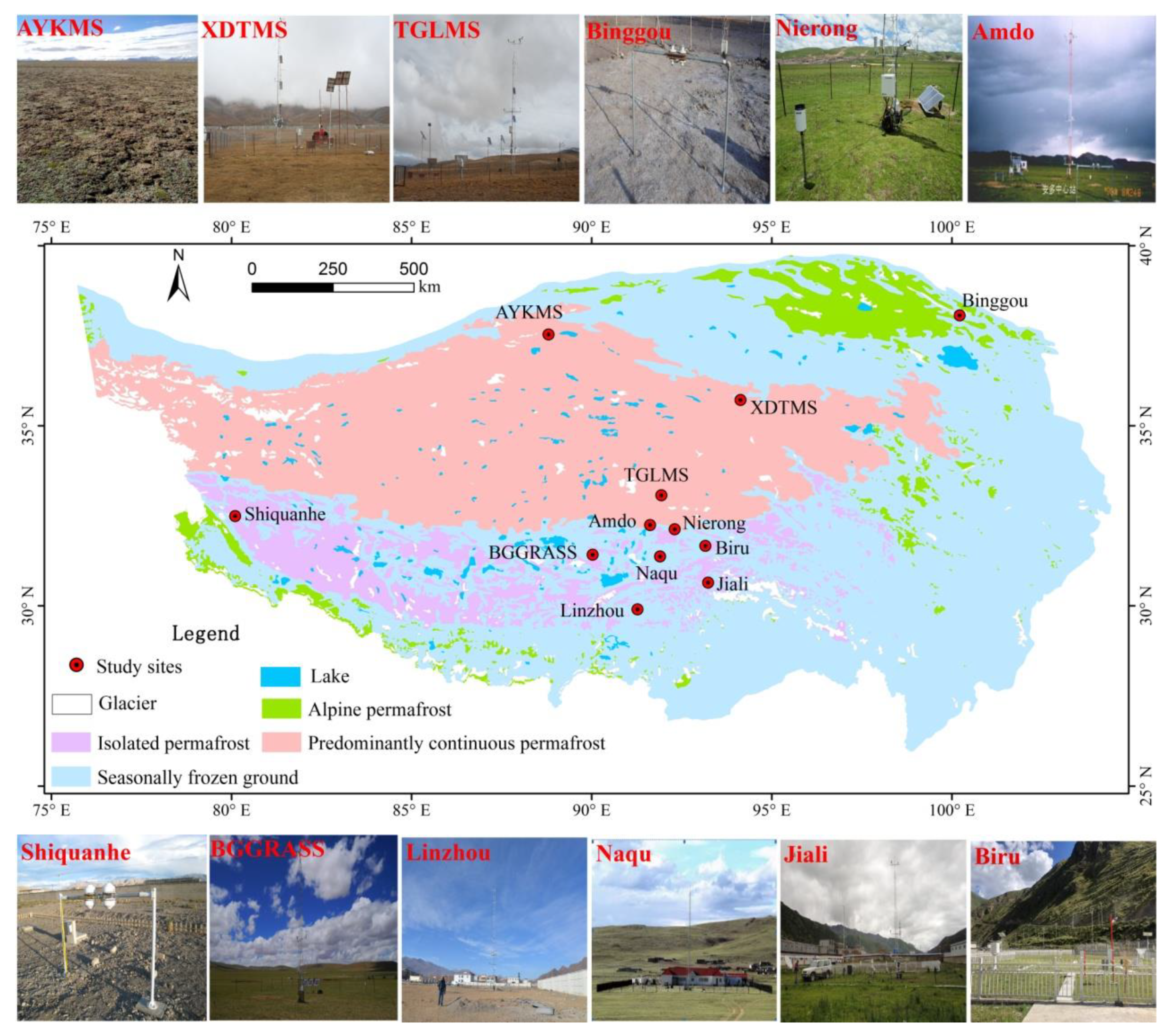
2.1. Study Regions

Observational data were collected from 12 automatic weather stations listed in Figure 1. This background map (Figure 1) shows the spatial distribution of frozen ground on the TP [25]. The Binggou site is located in the alpine meadow valley of the Binggou sub-basin in the upper reaches of the Heihe River. The east and west sides are continuous hills and mountains. The surrounding area is relatively flat and covered by a mixture of sparse grassland and riverbed gravel. The AYKMS site is located at the sparse desert grasslands of the boundary region between the permafrost and the seasonally frozen ground of the TP. The XDTMS sparse desert grasslands lie in the alpine steppe of the permafrost region near the northern lower limit of the permafrost on the TP. The TGLMS site is located in the alpine meadow of the predominantly continuous permafrost region. The observed area around the BGGRASS site is relatively flat and covered with alpine grassland, which is 2–4 cm tall. Alpine grassland is the main land surface type of Biru site. The Jiali site falls within the sub-frigid zone and semi-humid monsoon climate regions of the Plateau, with sufficient sunshine and strong radiation. The Naqu site is located in the alpine grassland of Naqu Valley and lies within the sub-frigid zone and semi-humid climate regions of Plateau [26]. The Nierong Site is affected by the terrain; the cold and dry climate falls within the sub-arid and semi-arid monsoon climate zone of Plateau. The terrain around the site is broad, expansive, and relatively flat and supports alpine meadow [27]. The Linzhou site is located in a valley surrounded by relatively flat of the alpine desert. Shiquanhe is located in the western part of the TP and has sparse and short grassland that is generally only a few centimeters tall. This part of the plateau experiences a cold zone monsoon arid climate. The solar radiation is strong with frequently strong surface wind speeds; the air is dry with less rain than other areas and experiences large daily temperature differences [28]. Amdo station has a relatively smooth surface with a very open view where sparse plateau meadow covers the ground.

2.2. Data Sources

2.2.1. In-Situ Measurement Data

The above 12 sites used in this study provided data for net radiation (R_n, downward/upward shortwave and longwave radiation), precipitation, soil temperature and humidity profiles, land surface temperature, and soil heat flux (

Table 1. Observational instruments and observation parameters.

AWS	Location (lon/lat/alt)	Ground Surface Condition	Observation Period (Beijing Time: dd.mm.yyyy)	Observation Items	Depth/Height
AYKMS	88°48′E 37°32′N 4300 m	Desert steppe	12.06.2014–24.02.2015	DSR/USR	2 m
				DLR/ULR	2 m
				G	5, 10, 20 cm
				SM	5, 10, 20, 40 cm
				ST	5, 10, 20, 40 cm
				Ts	1.5 m
				prec	1.5 m
TGLMS	91°56′E 33°04′N 5100 m	Alpine meadow	01.01–31.12.2015	DSR/USR	2 m
				DLR/ULR	2 m
				G	5, 10, 20 cm
				SM	35, 70, 105, 140, 175, 210, 245, 280, 300 cm
				ST	2, 5, 10, 20, 50, 70, 90, 105, 140, 175, 210, 245, 280, 300 cm
				Ts	1.5 m
				prec	1.5 m
XDTMS	94°08′E 35°43′N 4538 m	Alpine steppe	01.01.2015–31.12.2016	DSR/USR	2 m
				DLR/ULR	2 m
				G	5, 10, 20 cm
				SM	35, 70, 105, 140, 175, 210, 245, 280, 300 cm
				ST	2, 5, 10, 20, 50, 70, 90, 105, 140, 175, 210, 245, 280, 300 cm
				Ts	1.5 m
				prec	1.5 m
Binggou	100°13.31′E 38°4.05′N 3449.4 m	Alpine meadow	16.03–17.10.2008, 01.01–31.07.2009	DSR/USR	1.5 m
				DLR/ULR	1.5 m
				SM	5, 10, 20, 40, 80, 120 cm
				ST	5, 10, 20, 40, 80, 120 cm
				G	5, 15 cm
				prec	4.11 m
Amdo	91°37.2′E 32°14.4′N 4695 m	Alpine steppe	01.07.2014–30.09.2015	DSR/USR	1.5 m
				DLR/ULR	1.5 m
				SM	5, 10, 20, 40, 80, 160 cm
				ST	5, 10, 20, 40, 80, 160 cm
				G	5, 10 cm
				prec	1.5 m
BGGRASS	90°1.68′E 31°25.07′N 4700 m	Alpine steppe	15.07.2014–23.09.2015	DSR/USR	2 m
				DLR/ULR	2 m
				SM	5, 10, 20, 40, 100 cm
				ST	5, 10, 20, 40, 100 cm
				G	5, 10 cm
				prec	1.5 m
Biru	93°9.5′E 31°39.8′N 4408 m	Alpine steppe	14.09.2014–02.10.2015	DSR/USR	2 m
				DLR/ULR	2 m
				SM	5, 10, 20, 40, 100 cm
				ST	5, 10, 20, 40, 100 cm
				G	5, 10 cm
				prec	1.5 m
Jiali	93°13.95′E 30°38.456′N 4509 m	Alpine meadow	17.09.2014–28.06.2015, 06.09.2015–11.10.2015	DSR/USR	2 m
				DLR/ULR	2 m
				SM	5, 10, 20, 40, 100 cm
				ST	5, 10, 20, 40, 100 cm
				G	5, 10 cm
				prec	1.5 m
Naqu	91°54′E 31°22.2′N 4509 m	Alpine steppe	01.07–10.09.2014, 16.09–07.12.2014, 28.01–01.08.2015, 01.09–30.09.2015	DSR/USR	1.5 m
				DLR/ULR	1.5 m
				SM	5, 10, 20, 40, 80, 160 cm
				ST	5, 10, 20, 40, 80, 160 cm
				G	5, 10 cm
				prec	1.5 m
Nierong	92°18.27′E 32°7.33′N 4607 m	Alpine meadow	11.07.2014–21.10.2015	DSR/USR	1.5 m
				DLR/ULR	1.5 m
				SM	5, 10, 20, 50, 100 cm
				ST	5, 10, 20, 50, 100 cm
				G	5, 10 cm
				prec	1 m
Linzhou	91°16.25′E 29°53.93′N 3756 m	Alpine desert	19.09.2015–09.03.2016	DSR/USR	1.5 m
				DLR/ULR	1.5 m
				SM	5, 10, 20, 40, 80 cm
				ST	5, 10, 20, 40, 80 cm
				G	8 cm
				Ts	1.5 m
				prec	1.5 m
Shiquanhe	80°6′E 32°29.4′N 4278.6 m	Alpine desert	16.09.2014–30.09.2015	DSR/USR	2 m
				DLR/ULR	2 m
				SM	5, 10, 20, 40, 80 cm
				ST	5, 10, 20, 40, 80 cm
				G	5, 10, 20, 40, 80 cm
				Ts	1.5 m
				prec	1.5 m

NOTE: DSR, USR, DLR, and URL represent downward and upward shortwave radiation as well as downward and upward longwave radiation, respectively; T_s stands for land surface temperature; R_n represents net radiation; G is the soil heat flux; SM and ST stand for soil moisture and temperature, respectively; Prec is the precipitation.

). The data acquisition interval was 30 min. The observed data of the Binggou site were acquired from the Cold and Arid Regions Sciences Data Center (http://westdc.westgis.ac.cn/data/30617ca4-f46e-4254-a40a-5d0fbea58ed2). Meanwhile, the data for the AYKMS, TGLMS, and XDTMS sites were provided by the Cryosphere Research Station on the Qinghai-Tibet Plateau, Chinese Academy of Sciences (http://www.crs.ac.cn/), while the measured data of the other eight sites were downloaded from the National Meteorological Information Center (http://tipex.data.cma.cn/tipex). Precipitation data were used to eliminate data based on unusual weather. Soil heat flux, soil temperature, and soil moisture data were used to calculate G₀. Downward/upward shortwave radiation was used to calculate the land surface albedo in addition to R_n. In addition, R_n, land surface temperature, and land surface albedo acted as input parameters for the remote sensing-based models in estimating G₀.

Measured land surface temperature data (T_s) were unavailable for seven stations (Binggou, Amdo, BGGRASS, Biru, Jiali, Naqu, and Nierong), but the in-situ LST measurements were estimated from the upwelling and downwelling longwave radiation data using the Stefan–Boltzmann law [29,30]:

$$T_{\mathrm{s}}={\left[\frac{R_{\mathrm{L}}{}^{\uparrow }-\left(1-{\epsilon }_{\mathrm{s}}\right)\cdot R_{\mathrm{L}}{}^{\downarrow }}{{\epsilon }_{\mathrm{s}}\cdot \sigma }\right]}^{1/4}-273.15,$$

(1)

where T_s is the land surface temperature (unit: °C), R_L^↓ and R_L^↑ are the incoming and outgoing longwave radiation powers, respectively (unit: W/m²), σ is the Stefan–Boltzmann constant (5.67 × 10⁻⁸ W·m⁻²·K⁻⁴), and ε_s is the land surface emissivity, which is approximately 0.987 at Binggou [31] and 0.98 at the other six sites [32].

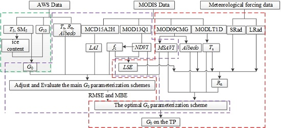
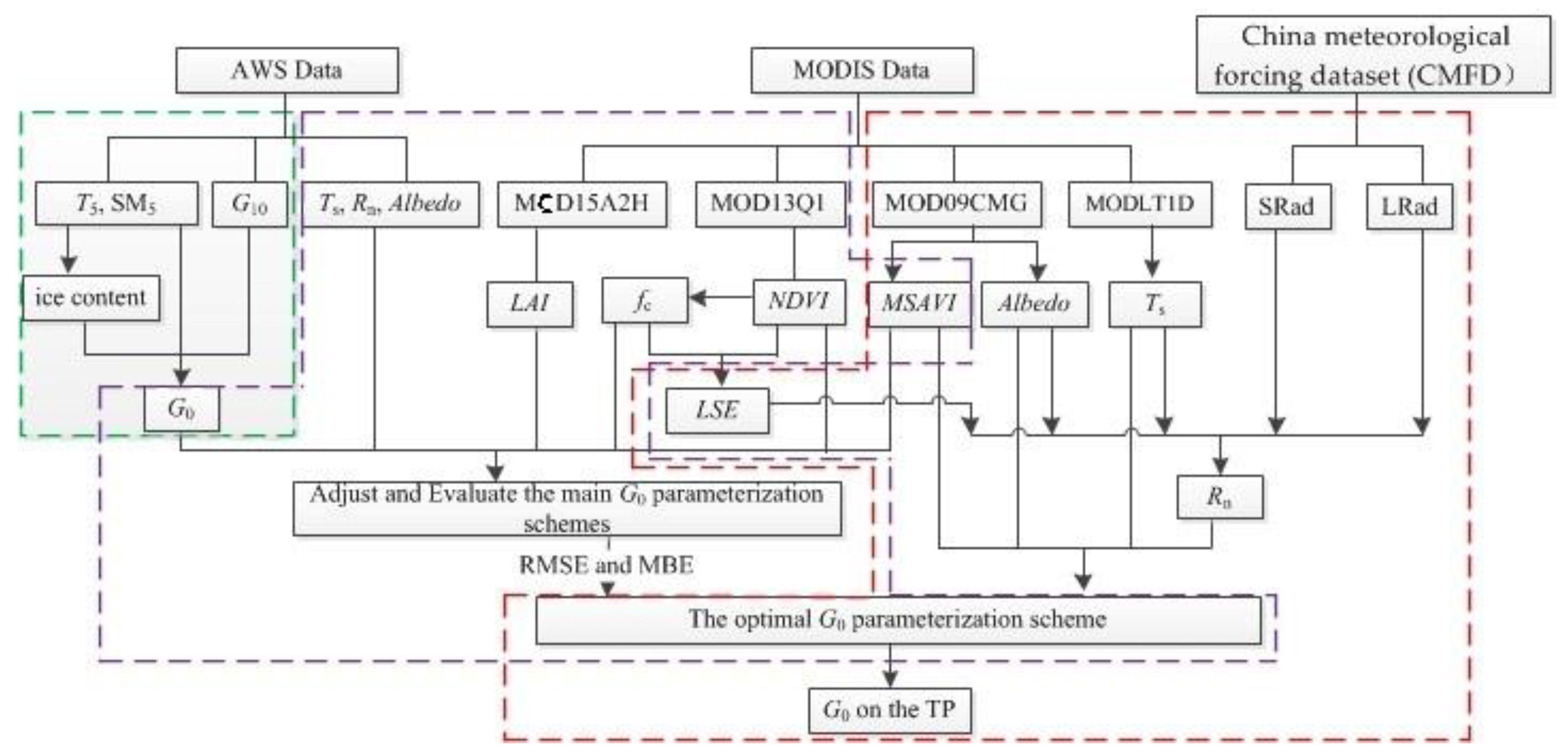
2.2.2. Remote Sensing Data (MODIS) and China Meteorological Forcing Dataset

Vegetation indices used in the study include NDVI, modified soil adjusted vegetation index (MSAVI), f_c, and LAI. These data were not observation-based but retrieved from remote sensing data (

Table 2. Specifications of Moderate Resolution Imaging Spectroradiometer (MODIS) products used in the study.

Product Name	Description	Time Range (Beijing Time: dd.mm.yyyy)	Time Granularity	Spatial Resolution
MOD13Q1	Normalized difference vegetation index (NDVI), enhanced vegetation index (EVI)	01.01.2008–31.12.2009, 01.01.2014–31.12.2016	16 day	250 m
MCD15A2H	Fraction of photosynthetically active radiation (FPAR), leaf area index (LAI)		8 day	500 m
MODLT1D	Daytime/Nighttime Land Surface Temperature	01.07–31.07.2014, 01.10–31.10.2014, 01.01–31.01.2015, 01.04–30.04.2015	Daily	1000 m
MOD09CMG	Surface reflectance band 1–7	24.07.2014, 25.10.2014, 21.01.2015, 26.04.2015	Daily	5600 m
CMFD-SRad	Downwelling shortwave radiation		3 h	10,000 m
CMFD-LRad	Downwelling longwave radiation		3 h	10,000 m

Note: MOD, Terra satellite’s MODIS data; MCD, combined data from all the acquisitions of both MODIS sensors located on NASA’s Terra and Aqua satellites.

). MODIS product MCD15A2H including LAI is an 8-day composite dataset with 500 m pixel size. The algorithm chooses the “best” pixel available from all the acquisitions of both MODIS sensors located on NASA’s Terra and Aqua satellites from within the 8-day period [33]. The NDVI data were obtained from the MODIS vegetation index product MOD13Q1; these data were produced on 16-day intervals and at 250 m spatial resolution. The modified soil adjusted vegetation index (MSAVI) was also calculated from the product MOD13Q1 by Equation (2) [34]:

$$MSAVI=\frac{2\cdot NIR+1-\sqrt{{\left(2\cdot NIR+1\right)}^2-8\cdot \left(NIR-RED\right)}}{2},$$

(2)

where RED and NIR are land surface reflectance values of RED and NIR bands of MOD13Q1, respectively. The fractional canopy coverage f_c can be obtained by NDVI [35]:

$$f\mathrm{c}={\left[\frac{NDVI-{NDVI}_{\min }}{{NDVI}_{\max }-{NDVI}_{\min }}\right]}^2,$$

(3)

where NDVI_max and NDVI_min are the NDVI values for bare soil and full vegetation, respectively.

The product MODLT1D was made using MOD11A1 through splicing, cutting, and projection conversion (http://www.gscloud.cn) with 1 km spatial resolution, provided along with the daytime and nighttime surface temperature bands associated using quality control assessments. The MOD09CMG product provides an estimate of the surface spectral reflectance of MODIS Bands 1 through 7, resampled to 5600 m pixel resolution and corrected for atmospheric conditions such as gasses, aerosols, and Rayleigh scattering.

China meteorological forcing dataset (CMFD, https://data.tpdc.ac.cn) developed by the Institute of Tibetan Plateau Research, Chinese Academy of Sciences, was used as the model input in this study. The dataset has merged the observations from 740 operational stations of the China Meteorological Administration with the corresponding Princeton Global Meteorological Forcing Dataset [36,37,38]. The parameters used in this study included downward shortwave (SRad) and downward longwave (LRad) radiation. These two parameters have a 10 km spatial resolution and a temporal resolution of 3 h (Table 2). All parameters provided or retrieved by MODIS data were converted to the same projection coordinate as CMFD datasets and resampled to 10 × 10 km. The transit time of the Terra satellite was local time 10:30 a.m., and TP was in the range of 75°E to 105°E (Beijing standard time 11:30–13:30); we chose the average values of CMFD corresponding to Beijing standard time 11:00 and 14:00.

3. Methods

Figure 2 shows the general steps used for deriving the G₀ in this paper. The green box demonstrates the process of calculating G₀ at sites based on the measured data (details in Section 3.1). The content in the purple irregular wireframe shows the process of adjusting and selecting the G₀ parameterization schemes (Section 3.2), and that in the red irregular wireframe presents the steps for estimating G₀ over the TP by the selected scheme using MODIS data and forcing datasets (Section 3.3).

3.1. Estimate G₀ at a Site

The G₀ estimation started with the soil 1-D heat conduction equation [7]:

$$\frac{\partial {\rho }_{\mathrm{s}}{c}_{\mathrm{s}}T}{\partial t}=\frac{\partial G}{\partial z}$$

(4)

$$G=k_{\mathrm{s}}\frac{\partial T}{\partial z},$$

(5)

where ρ_s is the soil density (unit: kg/m³), c_s is the soil specific heat (unit: J∙kg⁻¹∙K⁻¹), T is the soil temperature (unit: K), t is time (unit: s), z is the soil depth (unit: m, the downward direction is taken as positive), k_s is the soil heat conduction coefficient (unit: W∙K⁻¹∙m⁻¹), and G is the soil heat flux (unit: W/m², the direction down here is positive).

By integrating Equation (4), the G₀ is obtained:

$$G_0=G\left(z_{\mathrm{ref}}\right)+{\displaystyle {\int }_{z_{\mathrm{ref}}}^0\frac{\partial {\rho }_{\mathrm{s}}{c}_{\mathrm{s}}T}{\partial t}\mathrm{d}\mathrm{z}},$$

(6)

where z_ref is the reference depth (it was 0.10 m in this study), and G(z_ref) is the soil heat flux at the depth of the reference location.

For sites on the TP, there is a freeze-thaw process in the soil near the surface, so the ice thermal capacity should also be considered [7,39], so the discrete form of Equation (6) can be expressed as

$$G_0=G_{0.10\mathrm{m}}+\frac{\left({\rho }_{\mathrm{dry}}{c}_{\mathrm{dry}}+{\rho }_{\mathrm{w}}{c}_{\mathrm{w}}{\theta }_{0.05\mathrm{m}}+{\rho }_{\mathrm{i}}{c}_{\mathrm{i}}{\vartheta }_{\mathrm{i},0.05\mathrm{m}}\right)}{\partial t}\cdot 0.10,$$

(7)

where θ_0.05m is the unfrozen water content at 0.05 m depth (unit: m³∙m⁻³), ρ_dryc_dry is the thermal capacity of dry soil (about 0.90 × 10⁶ J∙m⁻³∙K⁻¹) [40], ρ_wc_w is the thermal capacity of liquid water (4.2 × 10⁶ J∙m⁻³∙K⁻¹), and ρ_ic_i is the ice thermal capacity (1.89 × 10⁶ J∙m⁻³∙K⁻¹). There were three different stages for the calculation of the soil ice content at 5-cm depth ϑ_i,0.05m:

(1) When the soil layer above 0.05 m was completely thawed, no ice existed in the layer (${\vartheta }_{i,0.05\mathrm{m}}=0$);

(2) When the daily freeze-thaw stage of the soil layer was above 0.05 m, the soil ice content ϑ_i,0.05m was approximately obtained by the difference of the steady unfrozen water content before and after the daily freeze-thaw stage of this soil layer. ϑ_i,0.05m can be calculated using Equation (8) [41]:

$$\frac{\partial {\rho }_{\mathrm{i}}\overline{{\vartheta }_{\mathrm{i},0.05\mathrm{m}}}}{\partial T}=\frac{\partial {\rho }_{\mathrm{w}}\overline{{\theta }_{0.05\mathrm{m}}}}{\partial T}$$

(8)

(3) When the soil layer above 5 cm was completely frozen, ϑ_i,0.05m equals the soil ice content of the last day of the daily freeze-thaw stage. It should be noted that the ice content was variable even if the soil was frozen, but such ice content variation was small in the frozen stages, so the ice content was approximately regarded as a constant during the frozen stages in the calculations [39]. The daily freeze-thaw stages were estimated based on the soil temperatures T_0.05m and unfrozen water contents θ_0.05m [39].

3.2. Introduction and Adjustments to G₀ Parameterization Schemes

3.2.1. Introduction and Adjustments to G₀ Parameterization Schemes

Several empirical remote sensing models can be used to estimate Γ(G₀/R_n), such as Choudhury [17], Clawson [15], SEBAL [13], Ma [19], and SEBS [18]. Choudhury et al. [17] expressed the relationship (the Choudhury scheme) between G₀ and R_n as an exponential function of the LAI with a correlation coefficient of 0.93:

$$G_0/R_{\mathrm{n}}=0.4\cdot {\mathrm{e}}^{0.5\cdot LAI}$$

(9)

A detailed description of the other four schemes is presented in

Table 3. The original and adjusted versions of remote sensing-based models estimating G₀/R_n.

Model Name	Mathematical Form	References
SEBAL	$G_0/R_{\mathrm{n}}=\frac{T_{\mathrm{s}}}{\alpha }\cdot (0.0062{\overline{\alpha }}^2+0.0028\overline{\alpha })\cdot (1-0.978NDV{I}^4)$	[13]
SEBALadj	$G_0/R_{\mathrm{n}}=\frac{T_{\mathrm{s}}}{\alpha }\cdot (0.006{\overline{\alpha }}^2+0.00258\overline{\alpha }+0.00112)\cdot (1-0.90NDV{I}^4)$	This study
Ma	$G_0/R_{\mathrm{n}}=\frac{T_{\mathrm{s}}}{\alpha }\cdot \left(0.0087{\overline{\alpha }}^2+0.0045\overline{\alpha }+0.00029\right)\cdot \left(1-0.964MSAV{I}^4\right)$	[19]
Maadj	$G_0/R_{\mathrm{n}}=\frac{T_{\mathrm{s}}}{\alpha }\cdot \left(0.0084{\overline{\alpha }}^2+0.0018\overline{\alpha }+0.00116\right)\cdot \left(1-0.96MSAV{I}^4\right)$	This study
Choudhury	$G_0/R_{\mathrm{n}}=0.4\cdot {{\displaystyle \mathrm{e}}}^{0.5\cdot LAI}$	[17]
Choudhuryadj	$G_0/R_{\mathrm{n}}=0.267\cdot {{\displaystyle \mathrm{e}}}^{0.27\cdot LAI}$	This study
Clawson	$G_0/R_{\mathrm{n}}=0.583\cdot {{\displaystyle \mathrm{e}}}^{-2.13\cdot NDVI}$	[42]
Clawsonadj	$G_0/R_{\mathrm{n}}=0.238\cdot {{\displaystyle \mathrm{e}}}^{0.78\cdot NDVI}$	This study
SEBS	$G_0/R_{\mathrm{n}}=\left[0.315\cdot \left(1-f_{\mathrm{c}}\right)+0.05\cdot f_{\mathrm{c}}\right]$	[18]
SEBSadj	$G_0/R_{\mathrm{n}}=\left[0.20\cdot \left(1-f_{\mathrm{c}}\right)+0.05\cdot f_{\mathrm{c}}\right]$	This study

Note: G₀, ground surface soil heat flux; R_n, net radiation; T_s, land surface temperature; α, instantaneous land surface albedo; $\overline{\alpha }$, daily mean land surface albedo; LAI, leaf area index; f_c, vegetation coverage; NDVI, normalized difference vegetation index; MSAVI, modified soil adjusted vegetation index.

of Yang et al. [23]. It should be noted that the Moran scheme is named the Clawson scheme in this study, which uses an exponential function of NDVI to the ratio of G₀/R_n [15,16]. In addition, Yang et al. [23] found that the ratio Γ_s of soil heat flux to net radiation for bare soil in the SEBS scheme should be less than 0.315 on the TP, which needs to be adjusted later.

SEBAL_adj, Ma_adj, Choudhury_adj, Clawson_adj, and SEBS_adj are the modified versions of the SEBAL, Ma, Choudhury, Clawson, and SEBS models, respectively (Table 3) and the modified versions of the five schemes are shown in Appendix A. So far, 10 schemes remain and need further discussion.

3.2.2. Indicators to Evaluate the Applicability of G₀ Parameterization Schemes

This study evaluates the applicability of each scheme over the TP from their errors and their sensitivity to land surface parameters during the freeze-thaw process.

The accuracies of the values produced by the models were evaluated using the root mean square error (RMSE) and mean bias error (MBE), defined as follows:

$$RMSE=\sqrt{\frac{{{\displaystyle \sum _{j=1}^m\left(P_j-G_j\right)}}^2}{m}}$$

(10)

$$MBE=\frac{{\displaystyle \sum _{j=1}^m\left(P_j-G_j\right)}}{m}$$

(11)

where P_j is the modeled value, G_j is the measured value, and m is the number of samples. We can choose the best one from the 10 models based on the RMSE and MBE.

These remote sensing-based schemes estimate G₀ based on the proportional relationship between G₀ and R_n. The difference between the schemes is that some models only use a vegetation index to estimate G₀/R_n, while others use land surface temperature and albedo as well as a vegetation index to estimate G₀/R_n. In addition, the net radiation R_n was obtained through Equation (13). The mathematical formulas of the schemes (Table 3) and Equation (13) were merged. It can be seen that their sensitivities to land surface temperature T_s, land surface albedo α, and the vegetation index VI (LAI, NDVI, MSAVI, and f_c) can be derived from the percentage change of simulated G₀ values when increasing or reducing the observed T_s by 1 K, the measured α by 0.02, or VI by 0.1 [43]:

$$\{\begin{array}{c}V{R}_{+\mathrm{accuracy}}=\frac{{\displaystyle \sum _{\mathrm{j}=1}^N\left|G_{+\mathrm{accuracy}}-G_{\mathrm{base}}\right|}}{N}\\ V{R}_{-\mathrm{accuracy}}=\frac{{\displaystyle \sum _{\mathrm{j}=1}^N\left|G_{-\mathrm{accuracy}}-G_{\mathrm{base}}\right|}}{N}\\ \begin{array}{l}\\ \\ V{R}_{\mathrm{accuracy}}=\max \left\{V{R}_{+\mathrm{accuracy}},V{R}_{-\mathrm{accuracy}}\right\}\end{array}\end{array}$$

(12)

where VR_+accuracy and VR_−accuracy indicate the average change of simulated G₀ values by increasing and reducing the “observed” T_s by 1 K or the measured α by 0.02, respectively; VR_accuracy is the ultimate sensitivity coefficient; G_base is the simulated G₀ value from observed data corresponding to the unchanged land surface temperature T_s, unchanged land surface albedo α, and unchanged vegetation index. Meanwhile, G_+accuracy and G_−accuracy represent the simulated G₀ value when the “observed” T_s is increased or decreased by 1 K or the measured α is increased or decreased by 0.02 or remotely sensed VI is increased or decreased by 0.1, respectively. N is the number of samples.

3.3. Estimating Regional G₀ on the TP

We used the evaluation indices (RMSE and MBE) in Section 3.2 to select the optimal scheme on the TP and then obtain all the parameters by remote sensing data that were needed for the optimal scheme; these were input into the scheme to obtain the spatial distribution characteristics of G₀ on the TP. All schemes required the use of net radiation, land surface albedo, surface temperature, and vegetation index as inputs; the remote sensing inversion algorithm for the vegetation index was introduced in Section 2.2.2. Here, we only introduce the methods for obtaining the remaining land surface parameters by remote sensing and reanalyzed data.

The net radiation R_n can be obtained through Equation (13) [44]:

$$\begin{array}{c}{R}_{\mathrm{n}}=R_{\mathrm{S}}{}^{\downarrow }-R_{\mathrm{S}}{}^{\uparrow }+R_{\mathrm{L}}{}^{\downarrow }-R_{\mathrm{L}}{}^{\uparrow }\\ R_{\mathrm{S}}{}^{\uparrow }=\alpha \cdot R_{\mathrm{S}}{}^{\downarrow }\\ R_{\mathrm{L}}{}^{\uparrow }=\sigma \cdot {\epsilon }_{\mathrm{s}}\cdot T_{\mathrm{s}}{}^4+(1-{\epsilon }_{\mathrm{s}})\cdot R_{\mathrm{L}}{}^{\downarrow }\end{array}\}{R}_{\mathrm{n}}=(1-\alpha )\cdot R_{\mathrm{S}}{}^{\downarrow }+{\epsilon }_{\mathrm{s}}\cdot R_{\mathrm{L}}{}^{\downarrow }-\sigma \cdot {\epsilon }_{\mathrm{s}}\cdot T_{\mathrm{s}}{}^4$$

(13)

where R_S^↑ and R_S^↓ are the upwelling and downwelling shortwave radiation (W∙m⁻²), respectively, and R_L^↓ and R_L^↑ are the downwelling and upwelling longwave radiation (W∙m⁻²), respectively. The product MODLT1D can provide T_s (the scale-factor is 0.02 and the unit is Kelvin). The instantaneous value of land surface albedo α in the time range from 10:00 to 16:00 is approximately equal to the daily average value of land surface albedo $\overline{\alpha }$ on the same day [23]. In addition, the land surface instantaneous albedo α can be derived from bands 1–5 and band 7 data in the MODIS product MOD09CMG and an empirical Equation (14) [45]:

$$\begin{array}{c}\alpha =0.160\times R_1+0.291\times R_2+0.243\times R_3+0.116\times R_4\\ +0.112\times R_5+0.018\times R_7-0.0015\end{array}$$

(14)

The errors in MODIS land surface temperature measurements and land surface albedo estimated using Equation (14) and MOD/MYD09, are 1 K [46] and 0.02 [47], respectively. ε_s is the land surface emissivity, which was calculated using Equation (15) [48]:

$${\epsilon }_s=\{\begin{array}{c}0.973,NDVI<0.05\\ 0.986+0.004\cdot f_{\mathrm{c}},0.05\le NDVI\le 0.7\\ 0.99,NDVI>0.7\end{array}.$$

(15)

4. Results

4.1. Errors of the Schemes during the Freeze-Thaw Process

The errors of the models were evaluated by RMSE and MBE using the data from four sites (TGL, Naqu, Biru, and Nierong) of the verification group (Figure 3). The RMSE values of the 10 schemes (five original schemes and five corresponding adjusted schemes) were recorded in the three stages of a freeze-thaw cycle. We can see that, overall, the RMSE values of the adjusted schemes based on the measured data of the eight sites are smaller than those of the original schemes. This is particularly obvious for the Choudhury scheme. The RMSE of the adjusted Choudhury_adj scheme is significantly smaller than the original Choudhury scheme. This phenomenon once again shows that if measured data are used, it is best to re-determine the empirical coefficients in a remote sensing-based model based on the measured data and then use it to conduct related research.

The RMSE of each scheme was significantly different throughout the freeze-thaw cycle (Figure 3a); the RMSE values of the three stages are roughly presented as a whole: CF < DFT < CT. The order may depend on whether a particular scheme is better able to correctly capture the direction of G₀ when G₀ and R_n are different in the three phases. When the direction of G₀ and R_n is different (Table 6), the data volume of the three stages is CT > DFT ≈ CF, and the amount of analog data that can correctly capture the G₀ direction is CF > DFT > CT, which directly leads to the smallest RMSE in the CF stage and the largest RMSE in the CT stage. The MBE of the CT stage, whether overestimated or underestimated, is less than that of the other two stages, while the MBE values of the other two stages are near to each other (Figure 3b).

For convenience, we divided the schemes into two groups according to the factors considered in them. The first group of schemes simulates G₀/R_n value using a vegetation index alone (Choudhury, Clawson, SEBS, Choudhury_adj, Clawson_adj, and SEBS_adj). Meanwhile, the second group schemes are based on T_s, α, and a vegetation index (NDVI or MSAVI) to estimate the G₀/R_n value (SEBAL, Ma, SEBAL_adj, and Ma_adj). An individual one of the first group of schemes was slightly better in a certain stage of the freeze-thaw cycle, but overall, the RMSE values of the second group schemes was smaller (Figure 3a). Overall, the first group schemes simulations were obviously overestimated, and those of another group were weakly underestimated (Figure 3b). This study considers that the Ma_adj scheme is more suitable for estimating G₀ on the TP. In addition, MSAVI is more suitable for arid and semi-arid or high-elevation areas than NDVI [19,20,49]. The eight sites that determined the scheme not only are very evenly distributed on the TP but also include the main land surface and frozen ground types, which can represent the overall situation of the TP; the RMSEs of the schemes in any of the three stages (CF, DFT, and CM) were also relatively close with a minimum of difference. If no measured data are available, the Ma_adj scheme can be considered for direct use on the TP.

4.2. Regional G₀ on the TP

This study mainly focused on the applicability of the G₀ parameterization scheme on the TP during the freeze-thaw cycle. Due to data limitations, this study selected the day with the largest proportion of valid data per month during a four-month period (July and October 2014, January and April 2015) to show the simulated G₀ by the scheme Ma_adj during the freeze-thaw cycle. We selected the four days (July 24, 2014, October 25, 2014, January 21, 2015, and April 26, 2015) according to the quality control documents of the remote sensing land surface temperature product MODLT1D (Figure 4). The CMFD downward shortwave (CMFD-SRad) and longwave (CMFD-LRad) radiation data have proven to have reasonable accuracy with the in-situ measurements over the TP, which means that the two CMFD datasets can be used as model inputs [38]. The method to estimate net radiation R_n over the TP by regional data (MODIS products and CMFD datasets) is described in detail in Section 3.3. Although some data are missing, it can roughly reflect the seasonal differences of land surface temperature (Figure 5), net radiation (Figure 6), and ground surface soil heat flux (Figure 7) on the TP, which are higher in July, are lower in October and January, and become high again in April.

Due to the absence of both remote sensing and measured data and consideration of a spatial homogeneity (10 km), only 11 measured G₀(R_n) values corresponding to the simulated G₀(R_n) values were available. As shown in Figure 9a,b, the estimates of net radiation and ground surface soil heat flux show reasonable agreement with the in-situ measurements. The RMSEs for the net radiation flux and soil heat flux are 114.43 and 45.99 W/m². The RMSE (45.99 W/m²) obtained from the regional data (MODIS and CMFD) as the input of the scheme Ma_adj is close to that (Figure 3a) obtained from the measured data as the input of the scheme Ma_adj. The slope of the fitting line between “observed” and simulated G₀ values was slightly less than but very close to 1 (0.83; Figure 8b), This tells us there was a slight underestimation of the simulated results; The coefficient of determination R² is 0.87. These indicators (RMSE, MBE, and R²) indicate that satisfactory results can be obtained by using the Ma_adj scheme. It should be noted that some bias exists between the estimated G₀ and ground measurements. The causes of the scheme errors are analyzed in detail in Section 5.2.

5. Discussion

5.1. The Sensitivity of Remote Sensing-Based Schemes to Land Surface Parameters

According to the sensitivity analysis indexes in Section 3.2.2, the sensitivity values of three stages of freeze-thaw process of each scheme can be determined. The Choudhury scheme is used as an example to illustrate the sensitivity of this scheme to three surface parameters (

Table 4. VR_accuracy, the ultimate sensitivity coefficient, of the scheme Choudhury.

Choudhury	CT	DFT	CF
+α	2.19	2.45	3.15
−α	2.19	2.45	3.15
+α, +LAI	1.25	1.08	1.16
+α, −LAI	4.89	5.06	6.04
−α, +LAI	5.25	5.44	6.51
−α, −LAI	1.25	1.07	1.11
+LAI	3.07	2.98	3.32
−LAI	2.92	2.84	3.16
+Ts	3.16	2.02	1.81
+Ts, +α	5.34	4.47	4.96
+Ts, −α	1.80	1.54	1.96
+Ts, +α, +LAI	3.27	2.37	2.35
+Ts, +α, −LAI	7.34	6.54	7.50
+Ts, −α, +LAI	4.33	4.45	5.30
+Ts, −α, −LAI	3.21	1.95	1.66
+Ts, +LAI	2.86	2.43	2.48
+Ts, −LAI	5.27	4.22	4.52
−Ts	3.12	2.00	1.79
−Ts, +α	1.79	1.54	1.96
−Ts, −α	5.31	4.45	4.94
−Ts, +α, +LAI	3.38	2.01	1.68
−Ts, +α, −LAI	4.05	4.17	4.96
−Ts, −α, +LAI	7.96	7.07	8.12
−Ts, −α, −LAI	2.84	2.05	2.02
−Ts, +LAI	5.66	4.51	4.82
−Ts, −LAI	2.68	2.32	2.39
MAX	7.96	7.07	8.12
N	11249	5171	5676

Note: The sign “+” (“−”) before T_s, α, or LAI represents that the parameter is increased (decreased) by 1 K, 0.02, or 0.1, respectively. N represents the number of samples. CF, DFT, and CT represent complete freezing stage, daily freeze-thaw cycle stage, and complete thawing stage of a freeze-thaw cycle, respectively.

). There are three cases for each land surface parameter: base + accuracy, base, and base − accuracy, so each scheme has 26 variations (3³–1 = 26, three to the third power indicates that there are three changes in each land surface parameter (+ accuracy, base, and − accuracy), and three land surface parameters (T_s, α, or VI) are considered in common; subtracting 1 is the case when three land surface parameters are all original values), where the largest VR value is used as VR_accuracy of the scheme.

The same idea is to get VR_accuracy of each scheme (

Table 5. VR_accuracy, the ultimate sensitivity coefficient, of these schemes.

Scheme	CT	DFT	CF
Choudhury	7.96	7.07	8.12
Choudhuryadj	3.60	3.70	4.28
Clawson	7.54	14.21	17.95
Clawsonadj	4.87	13.20	6.23
SEBS	8.89	22.52	29.57
SEBSadj	2.52	3.53	4.28
SEBAL	0.56	0.63	1.05
SEBALadj	1.61	1.47	1.69
Ma	0.88	1.11	1.68
Maadj	1.45	1.46	1.72

Note: CF, complete freezing; DFT, daily freeze-thaw cycle; CT, complete thawing.

); we know that, overall, these schemes that are based on T_s, α, and VI are more stable than others based on only VI. That is, when remotely sensed products are used as input parameters of remote sensing-based schemes, the results simulated by the schemes based on T_s, α, and VI are more stable. In addition, VR_accuracy values of the adjusted schemes (Choudhury_adj, Clawson_adj, and SEBS_adj) based on the vegetation index are significantly reduced (Table 5), which tells us their simulated results are more stable than those of their original schemes (Choudhury, Clawson, and SEBS). The VR_accuracy values of the two adjusted schemes (SEBAL_adj and Ma_adj) are larger than that of the two original schemes (SEBAL and Ma), although the difference is still no more than 2 W/m², which shows that the two adjusted schemes are more sensitive to land surface parameters within acceptable limits.

5.2. Analysis of the Causes of the Scheme Errors

Through a review of previous research [13,15,17,18,19,23,38] and the above findings of the present study, we knew that remote sensing-based models can provide satisfactory simulation results, and their application is convenient and simple. However, some errors do occur in the modeled results. Here, we discuss the sources of error from the following four aspects:

Soil moisture has a certain effect on the G₀/R_n ratio. The existing studies confirmed that the variability in G₀/R_n on hourly timescales is partly caused by variations in soil moisture [50,51,52,53]. This dependence arises from the competing effects of changing evaporation rates and soil thermal conductivity as the soil dries [54]. The drier the soil, the larger the G₀/R_n [24]. In addition, a significant difference exists in soil moisture during a freeze-thaw cycle, with the smallest soil moisture in the CF stage and the largest in the CT stage (Figure 9). However, none of these schemes considered the effects of soil moisture directly, which will result in the production of some errors. Although T_s is sensitive to soil moisture [24], it cannot completely replace soil moisture. From this point of view, the schemes considering T_s also have more advantages.

The phase shift between G₀ and R_n is also one of the sources of errors in all schemes. Some studies have shown that a phase shift exists between G₀ and R_n [23,24,54,55,56]. Ground surface soil heat flux and net radiation flux do not have the same diurnal variation shape. The soil heat flux peak values are usually later than the net radiation flux peak values, which was not taken into account in these parameterizations. In the present study, taking the measured data of TGL station as an example, no matter which stage of the freeze-thaw process was analyzed, an obvious phase shift occurred between G₀ and R_n. That is, the peak value of diurnal variation in G₀ always arrived later than the peak value of diurnal variation in R_n (Figure 10). Relevant studies have also been conducted on the TP, which concluded that the scheme considering the phase shift between G₀ and R_n does have a lower estimated error than before in the CT stage [23].

These remote sensing-based models are all based on G₀/R_n, so when the G₀ and R_n directions are opposite, the simulation results of each scheme are not very good.

Table 6. Simulation effect of each scheme on the direction of ground surface soil heat flux (G₀) when G₀ is the opposite direction from net radiation (R_n).

Scheme		CT	DFT	CF
G0 is the opposite direction from Rn		5102	2117	2270
Under the premise that G0 is opposite to Rn, the simulated G0 direction is consistent with the “measured” G0	Choudhury	0	0	0
	Choudhuryadj
	Clawson
	Clawsonadj
	SEBS
	SEBSadj
	SEBAL	853	1127	2051
	SEBALadj
	Ma
	Maadj

Note: The numbers in the table represent the number of samples; CF, DFT, and CT represent complete freezing stage, daily freeze-thaw cycle stage, and complete thawing stage of a freeze-thaw cycle, respectively.

shows that when G₀ has an opposite trend to that of R_n, the vegetation index-based scheme basically cannot correctly capture the direction of G₀. In contrast, the schemes that are based on T_s, α, and VI can reflect the direction of part of G₀ correctly and were used in the three stages of the freeze-thaw cycle. Here, G₀ manifests the energy exchange between the active layer and the atmosphere while it affects the energy budget of the active layer and permafrost, so its direction is crucial for the active layer thickness and permafrost [23]. When the direction of G₀ is positive (the downward direction of G₀ is positive), this finding indicates that the active layer absorbs heat from the atmosphere [56]. Over time, soil temperature will rise, which will increase the thickness of active layer and promote the degradation of permafrost. Vice versa, the active layer releases heat into the atmosphere [56], and the decrease of soil temperature is beneficial to the preservation and development of permafrost. Considering the correctness of the G₀ direction, although all schemes cannot fully capture the direction of G₀, a scheme based on T_s, α, and VI is better than a scheme based on vegetation index alone.

Remote sensing data will result in certain errors as presented in Table 5. Although the table shows the uncertainty of each scheme, it also shows the influence of an increase or decrease in the accuracy of remotely sensed land surface temperature, surface albedo, and vegetation indices on the simulated G₀; therefore, the accuracy of remotely sensed products has a certain effect on the simulation results of the main schemes.

6. Conclusions

Based on the observed TP and vegetation index data of 12 sites obtained from remote sensing products, we modified five remote sensing-based models to estimate the ground surface soil heat flux on the Tibetan Plateau during the freeze-thaw process and obtained 10 schemes (five original schemes and five modified schemes). We further analyzed RMSE values of 10 schemes, their sensitivity to land surface parameters, and the sources of their errors. The following conclusions are drawn.

(1)

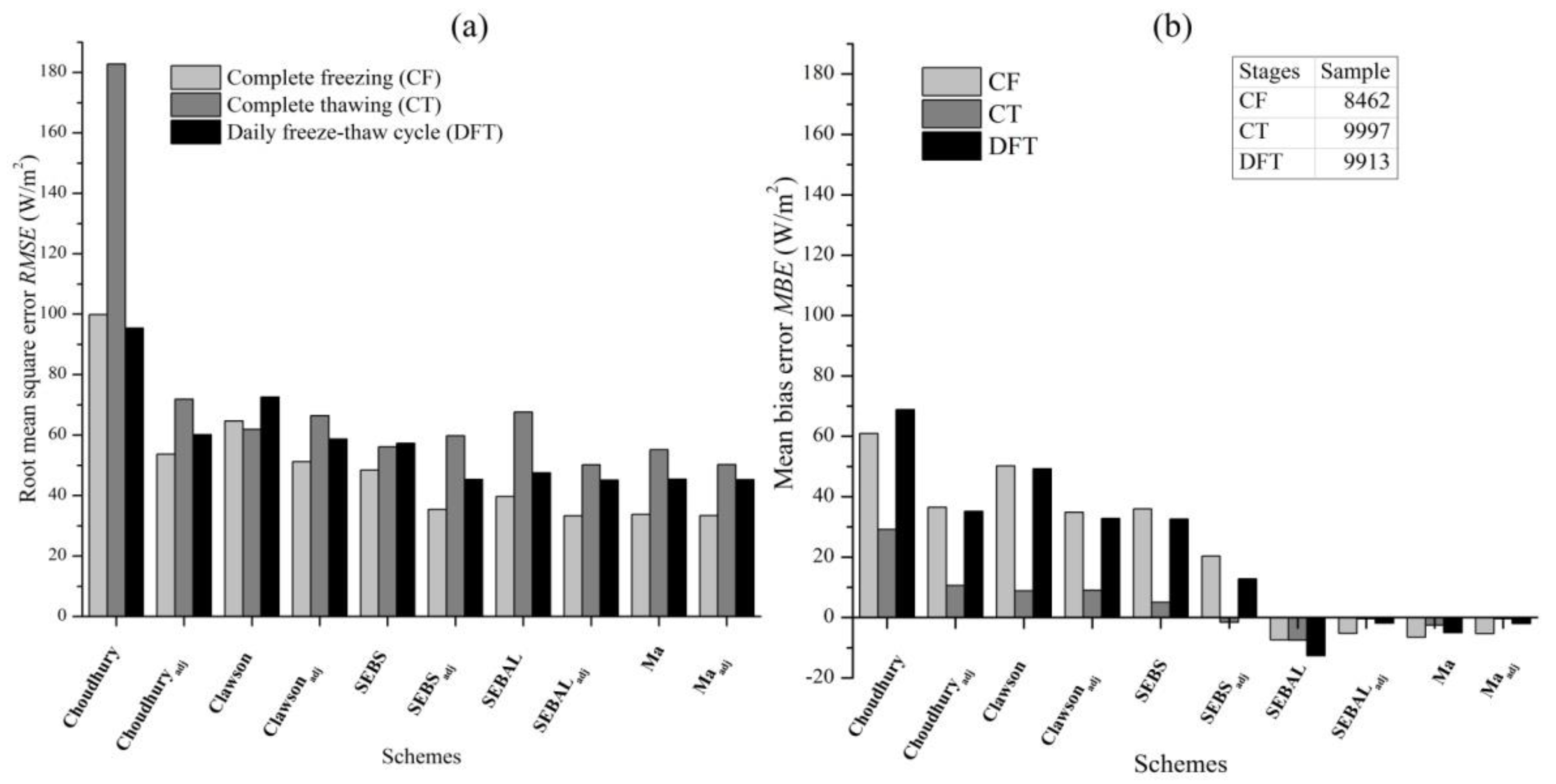
The RMSE of each scheme was significantly different during the freeze-thaw cycle on the TP; meanwhile, the RMSE values of the three stages can be roughly presented as a whole: CF < DFT < CT. The MBE of the CT stage, whether overestimated or underestimated, was less than that of the other two stages, while the MBE values of the other two stages were close. Overall, RMSE values of the second group of schemes (SEBAL, Ma, SEBAL_adj, and Ma_adj) were smaller than that of the first group of schemes (Choudhury, Clawson, SEBS, Choudhury_adj, Clawson_adj, and SEBS_adj). The MBE values tell us the G₀ values simulated by the first group of schemes were obviously overestimated, and those of the second group of schemes are weakly underestimated.

(2)

In the absence of measured data, the Ma_adj scheme can be considered for estimating G₀ on the TP; its RMSE and MBE were the least among all the schemes.

(3)

AV_accuracy of the second group of schemes was less and their simulated results were relatively more stable than those of the first group of schemes during the freeze-thaw process on the TP.

(4)

We discussed four possible reasons for the errors of the main schemes. Soil moisture, the phase difference between G₀ and R_n, whether each main scheme can correctly capture the propagation direction of G₀, and the accuracy of remote sensing data resulted in errors for the scheme analog results.

References

1. Ma, W.; Ma, Y.; Hu, Z.; Li, M.; Sun, F.; Gu, L.; Wang, J.; Qian, Z. The contrast between the radiation budget plus seasonal variation and remote sensing over the northern Tibetan Plateau. J. Arid Land Resour. Environ. 2005, 19, 109–115. [Google Scholar]
2. Xiao, Y.; Zhao, L.; Li, R.; Yao, J. Seasonal variation characteristics of surface energy budget components in permafrost regions of northern Tibetan Plateau. J. Glaciol. Geocryol. 2011, 33, 1033–1039. [Google Scholar]
3. Ye, D.; Gao, Y. Meteorology of Qinghai-Tibet Plateau; Science press: Beijing, China, 1979. [Google Scholar]
4. Wu, G. Recent progress in the study of the Qinghai-Xizang Plateau climate dynamics in China. Quat. Sci. 2004, 24, 1–9. [Google Scholar]
5. Shan, C.H.; Bo, S.Z. Simulation of Land-Atmosphere Exchange Processes at Amdo and Gaize Stations over Qinghai-Xizang Plateau. Plateau Meteorol. 2005, 24, 9–15. [Google Scholar]
6. Ma, Y.M.; Yao, T.D.; Wang, J.M. Experimental Study of Energy and Water Cycle in Tibetan Plateau—The Progress Introduction on the Study of GAME/Tibet and CAMP/Tibet. Plateau Meteorol. 2006, 25, 344–351. [Google Scholar]
7. Yang, K.; Wang, J. A temperature prediction-correction method for estimating surface soil heat flux from soil temperature and moisture data. Sci. China Ser. D 2008, 51, 721–729. [Google Scholar] [CrossRef]
8. Li, S.X.; Nan, Z.; Lin, Z. Impact of Soil Freezing and Thawing Process on Thermal Exchange between Atmosphere and Ground Surface. J. Glaciol. Geocryol. 2002, 24, 506–511. [Google Scholar]
9. Yang, M.X.; Yao, T.; Hirose, N.; Fujii, H. Diurnal freezing-thawing cycle of topsoil in Qinghai-Tibet Plateau. Chin. Sci. Bull. 2006, 51, 1974–1976. [Google Scholar]
10. Guo, D.L.; Xue, Y.M.; Min, L.; Peng, Q. Analysis on Simulation of Characteristic of Land Surface Energy Flux in Seasonal Frozen Soil Region of Central Tibetan Plateau. Plateau Meteorol. 2009, 28, 978–987. [Google Scholar]
11. William, P.J.; Smith, M.W. The Frozen Earth: Fundamentals of Geocryology; Cambridge University Press: Cambridge, UK, 1989. [Google Scholar]
12. Xu, Z.W.; Liu, S.M.; Xu, T.R.; Ding, C. The observation and calculation method of soil heat flux and its impact on the energy balance closure. Adv. Earth Sci. 2013, 28, 875–889. [Google Scholar]
13. Bastiaanssen, W.G.M. SEBAL-based sensible and latent heat fluxes in the irrigated Gediz Basin, Turkey. J Hydrol. 2000, 229, 87–100. [Google Scholar] [CrossRef]
14. Wang, J.M.; Ma, Y.M.; Menenti, M.; Bastiaanssen, W.; Mitsuta, Y. The scaling-up of processes in the heterogeneous landscape of HEIFE with the aid of satellite remote sensing. J. Meteorol. Soc. Jpn. 1995, 73, 1235–1244. [Google Scholar] [CrossRef] [Green Version]
15. Jackson, R.D.; Moran, M.S.; Gay, L.W.; Raymond, L.H. Evaluating Evaporation from Field Crops Using Airborne Radiometry and Ground-Based Meteorological Data. Irrig. Sci. 1987, 8, 81–90. [Google Scholar] [CrossRef]
16. Moran, M.S.; Jackson, R.D.; Raymond, L.H.; Gay, L.W.; Slater, P.N. Mapping surface energy balance components by combining Landsat thermatic mapper and ground-based meteorological data. Remote Sens. Environ. 1989, 30, 77–87. [Google Scholar] [CrossRef]
17. Choudhury, B.J.; Bjso, S.B.; Rejinato, R.J. Analysis of an empirical model for soil heat flux under a growing wheat crop for estimating evaporation by an infrared-temperature based energy balance equation. Agric. For. Meteorol. 1987, 39, 283–297. [Google Scholar] [CrossRef]
18. Su, Z. The Surface Energy Balance System (SEBS) for estimation of turbulent heat fluxes. Hydrol. Earth Syst. Sci. 2002, 6, 85–100. [Google Scholar] [CrossRef]
19. Ma, Y.M.; Ishikawa, H.; Tsukamoto, O.; Menenti, M.; Su, Z.B.; Yao, T.D.; Koike, T.; Yasunari, T. Regionalization of surface fluxes over heterogeneous landscape of the Tibetan Plateau by using satellite remote sensing data. J. Meteorol. Soc. Jpn. 2003, 81, 277–293. [Google Scholar] [CrossRef] [Green Version]
20. Ma, Y.M.; Wang, J.M.; Huang, R.H.; Wei, G.; Menenti, M.; Su, Z.B.; Hu, Z.Y.; Gao, F.; Wen, J. Remote sensing parameterization of land surface heat fluxes over arid and semi-arid areas. Adv. Atmos. Sci. 2003, 20, 530–539. [Google Scholar]
21. Ma, Y.M.; Ma, W.Q.; Li, M.S.; Sun, F.L.; Wang, J.M. Remote Sensing Parameterization of Land Surface Heat Fluxes over the Middle Reaches of the Heihe River. J. Desert Res. 2004, 24, 392–399. [Google Scholar]
22. Ma, Y.M.; Xue, D.Y.; Ma, W.Q.; Li, M.S.; Wang, J.M.; Wen, J.; Sun, F.L. Satellite Remote Sensing Parameterization of Regional Land Surface Heat Fluxes over Heterogeneous Surface of Arid and Semi-Arid Areas. Plateau Meteorol. 2004, 23, 139–146. [Google Scholar]
23. Cheng, Y.; Wu, T.; Wang, J.; Yao, J.; Li, R.; Zhao, L.; Xie, C.; Zhu, X.; Ni, J.; Hao, J. Estimating Surface Soil Heat Flux in Permafrost Regions Using Remote Sensing-Based Models on the Northern Qinghai-Tibetan Plateau under Clear-Sky Conditions. Remote Sens. 2019, 11, 416. [Google Scholar]
24. Min, W. Analysis of adaptabilities of remote sensing models for heat flux over hilly land. Sci. Meteorol. Sin. 2009, 29, 386–389. [Google Scholar]
25. Cheng, W.M.; Zhao, S.M.; Zhou, C.H.; Chen, X. Simulation of the Decadal Permafrost Distribution on the Qinghai-Tibet Plateau (China) over the Past 50 Years. Permafr. Periglac. Process. 2012, 23, 292–300. [Google Scholar]
26. Zhu, Z.K.; Hu, Z.Y.; Ma, Y.M.; Li, M.S.; Sun, F.L. Net ecosystem carbon dioxide exchange in alpine meadow of Nagchu region over Qinghai-Xizang Plateau. Plateau Meteorol. 2015, 34, 1217–1223. [Google Scholar]
27. Yang, L.W.; Gao, X.Q.; Hui, X.Y.; Gao, N.; Zhou, Y.; Hou, X.H. Study on turbulence characteristics in the atmospheric surface layer over Nyainrong grassland in central Qinghai-Tibetan Plateau. Plateau Meteorol. 2017, 36, 875–885. [Google Scholar]
28. Duan, L.J.; Duan, A.M.; Hu, W.T.; Gong, Y.F. Low frequency oscillation of precipitation and daily variation characteristic of air–land process at Shiquanhe station and Linzhi station in Tibetan Plateau in the summer of 2014. Chin. J. Atmos. Sci. 2017, 41, 767–783. [Google Scholar]
29. Yu, W.P.; Ma, M.G.; Wang, X.F.; Geng, L.Y.; Tan, J.L.; Shi, J.A. Evaluation of MODIS LST Products Using Longwave Radiation Ground Measurements in the Northern Arid Region of China. Remote Sens. 2014, 6, 11494–11517. [Google Scholar] [CrossRef] [Green Version]
30. Duan, S.B.; Li, Z.L.; Leng, P. A framework for the retrieval of all-weather land surface temperature at a high spatial resolution from polar-orbiting thermal infrared and passive microwave data. Remote Sens. Environ. 2017, 195, 107–117. [Google Scholar] [CrossRef]
31. Liu, S.M.; Xu, Z.W.; Wang, W.Z.; Jia, Z.Z.; Zhu, M.J.; Bai, J.; Wang, J.M. A comparison of eddy-covariance and large aperture scintillometer measurements with respect to the energy balance closure problem. Hydrol. Earth Syst. Sci. 2011, 15, 1291–1306. [Google Scholar] [CrossRef] [Green Version]
32. Wang, B.B.; Ma, Y.M.; Ma, W.Q. Estimation of land surface temperature retrieved from EOS/MODIS in Naqu area over Tibetan Plateau. J. Remote Sens. 2012, 16, 1289–1309. [Google Scholar]
33. Myneni, R.; Knyazikhin, Y.; Park, T. MCD15A2H MODIS/Terra+Aqua Leaf Area Index/FPAR 8-day L4 Global 500m SIN Grid V006. 2015. Available online: http://doi.org/10.5067/MODIS/MCD15A2H.006 (accessed on 1 February 2020).
34. Qi, J.; Chehbouni, A.; Huete, A.R.; Kerr, Y.H.; Sorooshian, S. A Modified Soil Adjusted Vegetation Index. Remote Sens. Environ. 1994, 48, 119–126. [Google Scholar] [CrossRef]
35. Carlson, T.N.; Ripley, D.A. On the relation between NDVI, fractional vegetation cover, and leaf area index. Remote Sens. Environ. 1997, 62, 241–252. [Google Scholar] [CrossRef]
36. He, J. Development of Surface Meteorological Dataset of Chinawith High Temporal and Spatial Resolution. Master’s Thesis, Inst. of Tibetan Plateau Res., Chin. Acad. of Sci., Beijing, China, 2010. [Google Scholar]
37. Yang, K.; He, J.; Tang, W.J.; Qin, J.; Cheng, C.C.K. On downward shortwave and longwave radiations over high altitude regions: Observation and modeling in the Tibetan Plateau. Agric. For. Meteorol. 2010, 150, 38–46. [Google Scholar] [CrossRef]
38. Zhong, L.; Ma, Y.M.; Hu, Z.Y.; Fu, Y.F.; Hu, Y.Y.; Wang, X.; Cheng, M.L.; Ge, N. Estimation of hourly land surface heat fluxes over the Tibetan Plateau by the combined use of geostationary and polar-orbiting satellites. Atmos. Chem. Phys. 2019, 19, 5529–5541. [Google Scholar] [CrossRef] [Green Version]
39. Yao, J.M.; Zhao, L.; Gu, L.L.; Qiao, Y.P.; Jiao, K.Q. The surface energy budget in the permafrost region of the Tibetan Plateau. Atmos. Res. 2011, 102, 394–407. [Google Scholar] [CrossRef]
40. Tanaka, K.; Tamagawa, I.; Ishikawa, H.; Ma, Y.M.; Hu, Z.Y. Surface energy budget and closure of the eastern Tibetan Plateau during the GAME-Tibet IOP 1998. J. Hydrol. 2003, 283, 169–183. [Google Scholar] [CrossRef]
41. Osterkamp, T.E. Freezing and Thawing of Soils and Permafrost Containing Unfrozen Water or Brine. Water Resour. Res. 1987, 23, 2279–2285. [Google Scholar] [CrossRef]
42. Jackson, R.D.; Pinter, P.J.; Reginato, R.J. Net-Radiation Calculated from Remote Multispectral and Ground Station Meteorological Data. Agric. For. Meteorol. 1985, 35, 153–164. [Google Scholar] [CrossRef]
43. Park, H.; Iijima, Y.; Yabuki, H.; Ohta, T.; Walsh, J.; Kodama, Y.; Ohata, T. The application of a coupled hydrological and biogeochemical model (CHANGE) for modeling of energy, water, and CO2 exchanges over a larch forest in eastern Siberia. J. Geophys. Res.-Atmos. 2011, 116. [Google Scholar] [CrossRef]
44. Amaty, P.M.; Ma, Y.M.; Han, C.B.; Wang, B.B.; Devkota, L.P. Recent trends (2003–2013) of land surface heat fluxes on the southern side of the central Himalayas, Nepal. J. Geophys. Res. Atmos. 2015, 120, 11957–11970. [Google Scholar] [CrossRef] [Green Version]
45. Liang, S.L. Narrowband to broadband conversions of land surface albedo I Algorithms. Remote Sens. Environ. 2001, 76, 213–238. [Google Scholar]
46. Wan, Z.M.; Li, Z.L. A physics-based algorithm for retrieving land-surface emissivity and temperature from EOS/MODIS data. IEEE Trans. Geosci. Remote Sens. 1997, 35, 980–996. [Google Scholar]
47. Liang, S.L.; Shuey, C.J.; Russ, A.L.; Fang, H.L.; Chen, M.Z.; Walthall, C.L.; Daughtry, C.S.T.; Hunt, R. Narrowband to broadband conversions of land surface albedo: II. Validation. Remote Sens. Environ. 2003, 84, 25–41. [Google Scholar] [CrossRef]
48. Qin, Z.L.; Li, W.J.; Xu, B.; Chen, Z.X.; Liu, J. The estimation of land surface emissivity for Landsat TM6. Remote Sens. Land Resour. 2011, 16, 28–32. [Google Scholar]
49. Ma, Y.M.; Tsukamoto, O.; Ishikawa, H.; Su, Z.B.; Menenti, M.; Wang, J.M.; Wen, J. Determination of regional land surface heat flux densities over heterogeneous landscape of HEIFE integrating satellite remote sensing with field observations. J. Meteorol. Soc. Jpn. 2002, 80, 485–501. [Google Scholar] [CrossRef] [Green Version]
50. Idso, S.B.; Aase, J.K.; Jackson, R.D. Net radiation–soil heat flux relations as influenced by soil water content variations. Bound.-Layer Meteorol. 1975, 9, 113–122. [Google Scholar] [CrossRef]
51. Fuchs, M.; Hadas, A. The heat flux density in a nonhomogeneous bare loessial soil. Bound.-Layer Meteorol. 1972, 3, 191–200. [Google Scholar] [CrossRef]
52. Clothier, B.E.; Clawson, K.L.; Pinter, P.J.; Moran, M.S.; Reginato, R.J.; Jackson, R.D. Estimation of Soil Heat-Flux from Net-Radiation during the Growth of Alfalfa. Agric. For. Meteorol. 1986, 37, 319–329. [Google Scholar] [CrossRef]
53. Ogee, J.; Lamaud, E.; Brunet, Y.; Berbigier, P.; Bonnefond, J.M. A long-term study of soil heat flux under a forest canopy. Agric. For. Meteorol. 2001, 106, 173–186. [Google Scholar] [CrossRef]
54. Santanello, J.A.; Friedl, M.A. Diurnal covariation in soil heat flux and net radiation. J. Appl. Meteorol. 2003, 42, 851–862. [Google Scholar] [CrossRef]
55. Colaizzi, P.D.; Kustas, W.P.; Anderson, M.C.; Agam, N.; Tolk, J.A.; Evett, S.R.; Howell, T.A.; Gowda, P.H.; O’Shaughnessy, S.A. Two-source energy balance model estimates of evapotranspiration using component and composite surface temperatures. Adv. Water Resour. 2012, 50, 134–151. [Google Scholar] [CrossRef] [Green Version]
56. Zhao, L.; Sheng, Y.; Wu, T.H.; Li, R.; Xie, C.W.; Wu, J.C.; Li, J.; Yao, J.M.; Wu, X.D.; Hu, G.J.; et al. Permafrost and Its changes on Qinghai-Tibet Plateau; Science press: Beijing, China, 2019. [Google Scholar]
Figure 1. Distribution of study sites on the Tibetan Plateau (source of permafrost distribution data: [25]) For abbreviations of site names and further details see Table 1.
Remotesensing 12 00501 g001
Figure 2. Flow chart used for estimating the ground surface soil heat flux (G0) on the Tibetan Plateau by combining Moderate Resolution Imaging Spectroradiometer (MODIS data, including MOD15A2H, MOD13Q1, MOD09CMG, and MODLT1D) and meteorological forcing data. Note: T5, soil temperature at a depth of 5 cm; SM5, 5 cm-depth soil moisture; G10, soil heat flux at a depth of 10 cm; Ts, land surface temperature; Rn, net radiation; Albedo, land surface albedo; LAI, leaf area index; fc, vegetation coverage; NDVI, normalized difference vegetation index; MSAVI, modified soil adjusted vegetation index; LSE, land surface emissivity; SRad, downward shortwave radiation; LRad, downward longwave radiation; G0, ground surface soil heat flux.
Remotesensing 12 00501 g002
Figure 3. Root mean square error (RMSE) (a) and mean bias error (MBE) (b) of each scheme at different stages (CF, complete freezing; DFT, daily freeze-thaw cycle; CT, complete thawing) of the freeze-thaw cycle. The table in the upper right corner in Figure 3b corresponds to the number of samples in the three stages.
Remotesensing 12 00501 g003
Figure 4. Fractions of valid moderate resolution imaging spectroradiometer land surface temperature data (Ts) on the Tibetan Plateau at 10:30 local time in July 2014, October 2014, January 2015, and April 2015 during the daytime.
Remotesensing 12 00501 g004
Figure 5. Spatial distribution of land surface temperature Ts at 10:30 local time on July 24 (a) and October 25 (b) in 2014, and January 21 (c) and April 26 (d) in 2015. Note: Ts stands for land surface temperature. The unit is kelvin.
Remotesensing 12 00501 g005
Figure 6. Spatial distribution of net radiation Rn at 10:30 local time on July 24 (a) and October 25 (b) in 2014, and January 21 (c) and April 26 (d) in 2015. Note: Rn stands for net radiation. The unit is W/m−2.
Remotesensing 12 00501 g006
Figure 7. Spatial distribution of ground surface soil heat flux G0 at 10:30 local time on July 24 (a) and October 25 (b) in 2014, and January 21 (c) and April 26 (d) in 2015. Note: G0 stands for ground surface soil heat flux. The unit is W/m−2.
Remotesensing 12 00501 g007
Figure 8. Validation of estimated net radiation (a) and ground surface soil heat flux (b) with in-situ measurements (The gray numbers (1–11) in Figure 8a,b represent the sites and dates corresponding to the red circles, shown in the table (c)). Note: RMSE, root mean square error; MBE, mean bias error; R2, the coefficient of determination.
Remotesensing 12 00501 g008
Figure 9. Changes of volumetric moisture content of unfrozen water in soil at 0.05 m depth during a freeze-thaw cycle at sites (a) Nierong, (b) TGLMS, (c) Naqu, and (d) Biru (CF, complete freezing; DFT, daily freeze-thaw cycle; CT, complete thawing).
Remotesensing 12 00501 g009
Figure 10. Schematic diagram of the phase shift between ground surface soil heat flux (G0) and net radiation (Rn) at site TGLMS during (a) complete freezing (CF), (b) complete thawing (CT), and (c) the daily freeze-thaw cycle (DFT) of a freeze-thaw process.
Remotesensing 12 00501 g010