Application of Beamforming Technology in Ionospheric Oblique Backscatter Sounding with a Miniaturized L-Array

Abstract

In this paper, a new dedicated multi-channel ionospheric oblique backscatter sounder is described. A miniaturized L-shaped antenna array was employed for the receiving of the oblique backscatter echoes in the present system. Firstly, two typical adaptive beamforming algorithms were introduced to improve the anti-jamming ability. Then, simulations were carried out to verify the beamforming performance in azimuth and elevation simultaneously. Furthermore, the experimental results by the present sounding system were used to test the performance of the adaptive beamformers. Results show that the radio frequency interference and the interference of the vertical echoes can be effectively suppressed by the adaptive beamformers. In particular, the use value of the beamforming in the receiving of the ionospheric oblique backscatter sounding is described in detail through the analysis of the signal sequences in several typical frequencies. And after the constant false-alarm rate processing, the oblique backscatter ionograms processed by the adaptive beamforers have clearer and continuous leading edge compared with the original ionograms. As a result, the adaptive beamformers of great significance to improve the detection ability of the ionospheric oblique backscatter sounding.

1. Introduction

High-frequency (HF) radio waves with frequencies between 3 and 30 MHz are an important frequency band for radar to sense the Earth’s environment [1]. Since the ionosphere can reflect HF radio waves, especially characteristics of its reflection characteristics are directly related to electron density in the ionosphere, HF radar sounding is one of the most important remote sensing means to study the ionosphere [2]. To date, a number of HF radars and ionospheric research programs have been developed and pursued for many applications, including the important contributions to validating the ionospheric models, investigating the HF radio communications, providing frequency management basis for over-the-horizon radars (OTHR) or tracking of earthquakes and so on [3,4,5,6,7]. These are all inseparable from the use of HF radar to detect the ionosphere.

The type of HF radar dedicated to the ionospheric sounding is often called an ionosonde. According to the incident mode and propagation route of the sounding signal, ionosonde can be divided into the oblique backscatter sounder, vertical-incidence sounder and oblique-incidence sounder [8,9,10]. Among them, the oblique backscatter sounding is a very unique method. The HF sounding signals emitted by the transmitter can be reflected by the ionosphere to the distant ground or the water surface, and a part of the backscattered signals return along the original path to the transmitting place. By receiving and analyzing these scattered signals, the oblique backscatter ionogram can be obtained. Due to the time focusing effect, there is a steep leadingier on the frequency-group delay map of the backscatter ionogram. By extracting the traces of the leadingier and performing inversions, a wide range of ionospheric states can be monitored, which is not available in other detection methods.

The conventional oblique backscatter sounder is mostly single channel, but the system with multi-channels has greater advantages. Employing the beam forming technology and the antenna array, directional detection can be realized and transmission power can be fully utilized. At present, some such systems have been built and widely recognized, such as Nostradamus OTHR, Jindalee sky-wave OTHR, and Super Dual Auroral Radar Network (SuperDARN), etc. [11,12]. Although they have good sounding performance, unfortunately, as OTHR, they are not dedicated oblique backscatter sounders. For ionospheric oblique backscatter sounding, it often exists only as a subsidiary function. To meet the capabilities required for OTHR tasks, they all rely on the large transmission power and antenna array. NOSTRADAMUS has a transmit power of 50 kW. The antenna array is Y-shaped and consists of 288 double-cone antennas. Each arm of the array is up to 400 m long [11]. Analogously, the total length of the 32 receiving sub-arrays of Jindalee is even 2.8 km long, and each of the 16 transmitting elements has a transmitting power of 20 kw [13]. Limited by the linear structure of the array, it can only perform azimuthal scanning. The main antenna array employed by SuperDARN also consists of 16 logperiodic antennas to scan at azimuth. The elevation information needs to be measured in conjunction with another subarray. Each transmitter has a peak output power ranging from 500–800 W [14].

The Ionospheric Laboratory of Wuhan University has conducted the research on the miniaturized but dedicated ionospheric oblique backscatter sounder system for a long time. Representatively, the Wuhan Ionospheric Oblique Backscatter Sounding System (WIOBSS) was developed in 2003 and constantly improved [15,16]. In 2016, Cui proposed a new generation of the WIOBSS system incorporating a logperiodic antenna array (WIOBSS-AA) [17]. However, because of the linear array, WIOBSS-AA does not support the two-dimensional (2-D) pointing in azimuth and elevation. In addition, as a test system, some beamforming technologies with better performance were not applied, and the advantages of multi-channel sounding system were also not been fully demonstrated. The processing effect of the beamformer on the oblique backscatter signals were also not analyzed in detail.

In this paper, a new dedicated multi-channel oblique backscatter sounder with a miniaturized L-shaped antenna array is described. Relaying on the high pulse compression gain of m-sequence, a 500 W transmission power can meet the sounding requirement. Some experiences were carried out to test the performance of the present system with adaptive beamforming algorithms.

Compared with existing systems or sounding methods, the main innovations of this paper are as follows:

• The system realized miniaturization design and is dedicated to ionospheric oblique backscatter sounding, which can provide real-time ionospheric state information.
• The system adopted two-dimensional directional receiving, which is more flexible and easier to adjust. Compared with the beamforming method of the transmitter, it has better anti-jamming ability at the receiver.
• The 2-D adaptive beamformer effectively suppressed the vertical echoes and other RF interferences.
• After adaptive beamforming processing, the leading edge of the oblique backscatter ionogram is clearer and steeper. It is of great significance for the trace extraction, which may further affect the inversion accuracy and improve the effective observation range.

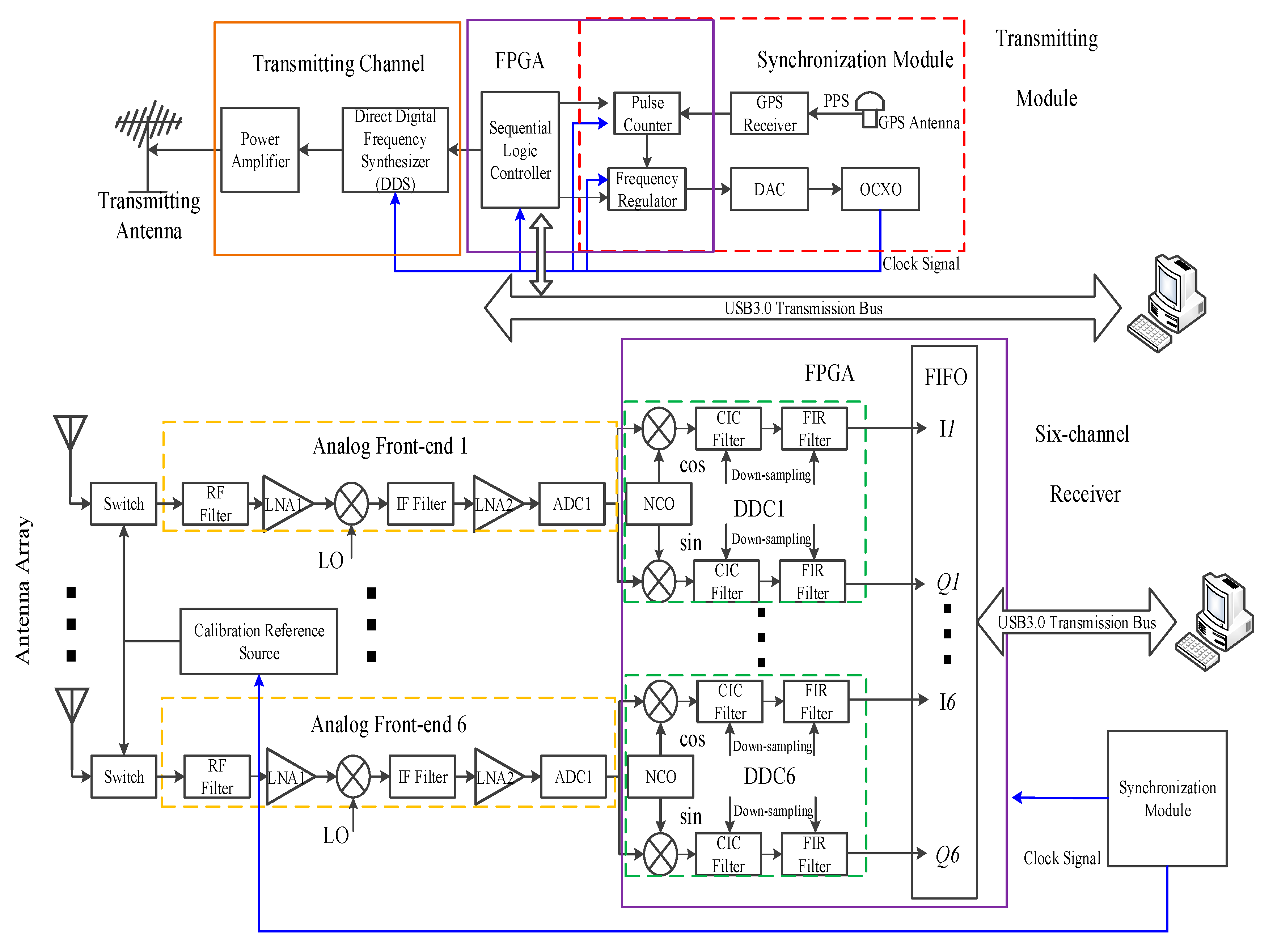
2. System Description

Unlike the WIOBSS-AA, we developed another system branch based on WIOBSS in 2018. The specific architecture is shown in Figure 1. The transmitter is a single channel subsystem. To obtain a large pulse compression gain, a sequence of pseudo-random code is employed as the modulating signal [18]. The multi-channel receiver has six independent channels. Correspondingly, six antennas form a miniaturized antenna array. In addition, a calibration reference source is included to ensure the amplitude and phase consistency of the channels. This system operates in the HF band (3–30 MHz), generally works in the frequency step scan mode for the oblique backscatter sounding. In order to make full use of the transmitting power, the system adopts the modulated continuous wave for transmitting. This will cause serious interference in the near field of the transmitting end. Thus, the receiving and transmitting subsystems are set up in different places. To ensure the time-frequency synchronization of them, synchronization modules are included by both.

2.1. Transmitting Subsystem

The function of the transmitting subsystem is to produce the modulated RF waveforms according to the set program. The transmitting subsystem is mainly composed of the synchronization module, a sequential logic controller built in a Field-Programmable Gate Array (FPGA) device, and a signal synthesis and amplification channel. Among them, the synchronization module calibrates the Oven Controlled Crystal Oscillator (OCXO) with the standard Pulses Per Second (PPS) signal provided by Global Positioning System (GPS). The logic part of the synchronization module is implemented in FPGA, nested with the sequential logic controller. The output frequency of OCXO can be adjusted according to the voltage on the specific pin. A chip of Direct Digital Synthesizer (DDS) generate the sounding waveform based on the parameters given by the sequential logic controller. After amplified by the power amplifier, the sounding signal with an appropriate power will be fed into the transmitting antenna.

The transmitting channel, power amplifier and transmitting antenna are shown in Figure 2. The transmitting channel is packaged in an aluminum alloy mold to shield interference and ensure the purity of the transmitting waveform. An amplifier with a maximum transmitting power of 500 W is adopted. The transmitting antenna is a Log-Periodic Dipole Antenna (LPDA) consists of 18 dipole elements with a boom length of approximately 14 m, and the longest dipole element is almost 15 m long. The main lobe of the antenna points to 113° north by east. In elevation angle, the width of the lobe is relatively large. In the following analysis and experiment, we choose $(\phi ={113}^{\circ },\theta ={35}^{\circ })$ cover the incident area of the desired signals with low elevations.

2.2. Multi-Channel Receiver

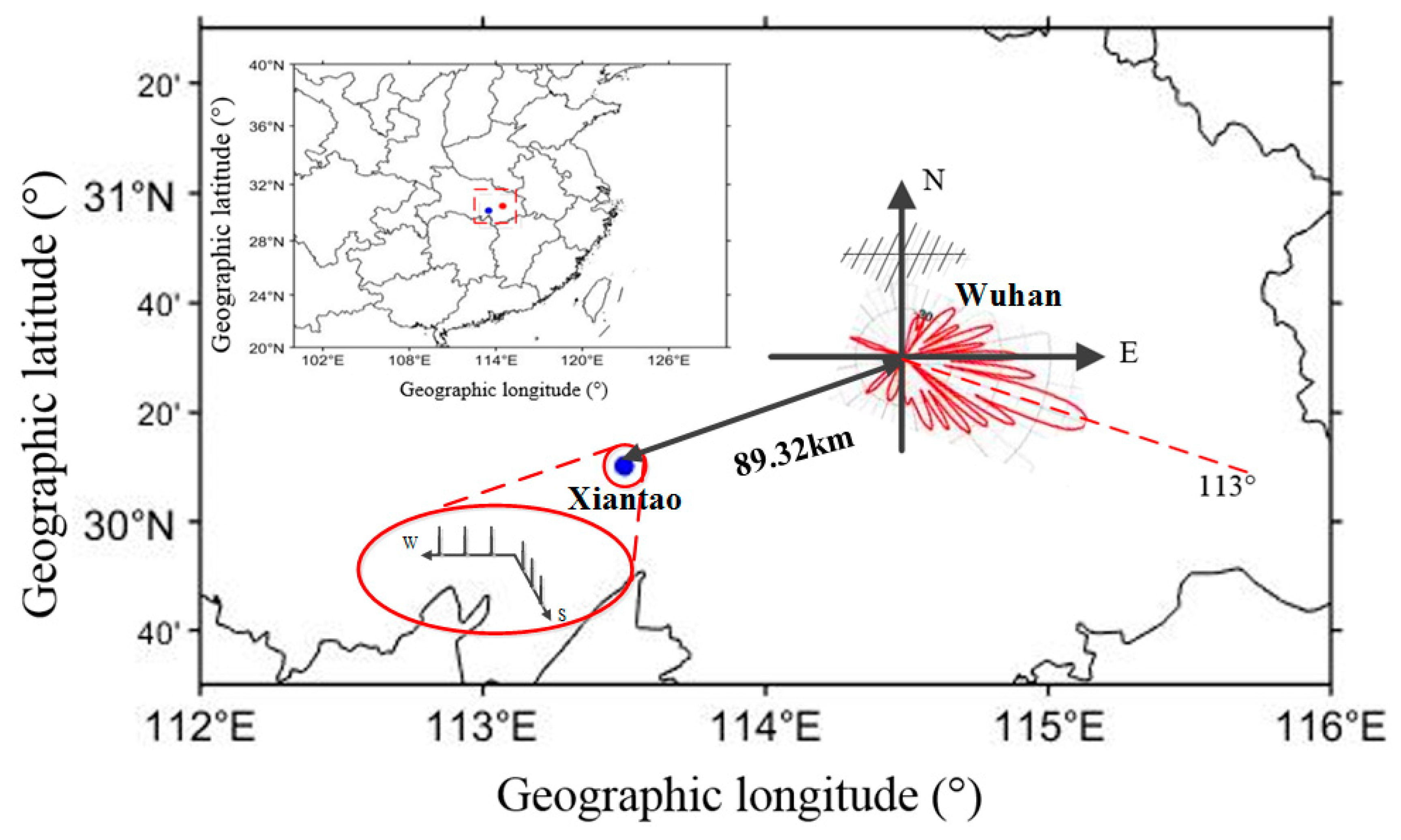
The multi-channel receiver contains six channels adopting digital the intermediate frequency (IF) architecture. It is mainly composed of the analog leading-ends and the Digital Down Conversion (DDC) modules integrated in FPGA. In the analog leading-ends, after being filtered and amplified, the signals are mixed to IF of 71.4 MHz. Then, the sampled signals are extracted in DDC, down converted to zero IF and reduced the data rate to baseband through downsampling. The calibration reference signal source ensures the beamforming accuracy by feeding the reference signal into every receiving channel to calculate the amplitude and phase errors. The synchronization module ensures the time-frequency synchronization with the transmitting subsystem.

The overall structure of the receiver, the boards of the analog leading-ends, Analog-to-Digital Converter (ADC) and DDC are shown in Figure 3. Each module is packaged in a separate aluminum mold, which effectively reduces external interference and ensures isolation between the channels. The whole receiver is packaged in a 2-Unit case, which is very compact and easy to transfer.

2.3. Antenna Array

In general, 2-D beamforming applications, the antenna array is usually arranged as a plane array or a circular array, which can facilitate good pointing performance. The array of NOSTRADAMUS can also be seen as a type of plane array. However, the plane array needs much more antennas to play its advantages, while the circular array needs a large area of site but with low utilization rate. Although the pointing ability of L-array is not as good as the first two, it is very suitable for the miniaturized system proposed in this paper. In addition to the ability to realize 2-D directional sounding, the hardware cost and site requirements are much lower.

In our system, six 6-m whip antennas form the receiving array in L-shaped. In addition to beamforming, it can also be employed angle of arrival (AOA) estimation in some other applications. The layout and actual scene are shown in Figure 4. Unlike the usual L-array, there are three antennas in each baseline along the east-west and the south-north but with no antenna in the intersection. In this way, the antenna array has the same performance in two orthogonal directions. The antennas and receiving channels are also utilized to the maximum extent.

To facilitate the analysis, we define the true north as the x-axis, which is also the reference direction. The azimuth $\phi$ is defined with the clockwise direction (rotating to the East, y-axis) as positive. With the ground as a reference, the elevation is defined as $\theta$. Thus, for the receiving array, when the intersection point O is defined as the reference point, the array manifold $a(\theta ,\phi )$ can be expressed as Equation (1).

$$\{\begin{array}{l}a(\theta ,\phi )=\left[\begin{array}{c}{a}_x(\theta ,\phi )\\ a_y(\theta ,\phi )\end{array}\right]\\ a_x(\theta ,\phi )={[e^{-2j\pi •d_x\sin \phi \cos \theta /\lambda },e^{-2j\pi •2d_x\sin \phi \cos \theta /\lambda },e^{-2j\pi •3d_x\sin \phi \cos \theta /\lambda }]}^T\\ a_y(\theta ,\phi )={[e^{-2j\pi •d_y\cos \phi \cos \theta /\lambda },e^{-2j\pi •2d_y\cos \phi \cos \theta /\lambda },e^{-2j\pi •3d_y\cos \phi \cos \theta /\lambda }]}^T\end{array}$$

(1)

where $a_x$ and $a_y$ are the flow pattern of the subarray on the x-axis and y-axis. $dx$ and $dy$ are the spacing between two adjacent antennas of the two axes. $\lambda$ is the wavelength of the currently operating frequency. In order to ensure that there are no grating lobes generated in the frequency band of 5–15 MHz in the experiment described below, we choose $dx=dy=10\mathrm{m}$.

3. Beamforming of the Miniaturized L-Array

The manifold of the array describes the phenomenon that the sampling signals of the adjacent receiving elements have phase difference due to the different spatial positions. This phase difference is determined by the spatial positions of the elements and the incident direction of the signal. Clearly, if the signals of every channel are added directly, interference weakening will occur except in the direction of vertical upward. In essence, beamforming is to eliminate the phase difference according to the pointing direction, thus the signals of each channel can be added in the same phase to get higher quality in a particular direction.

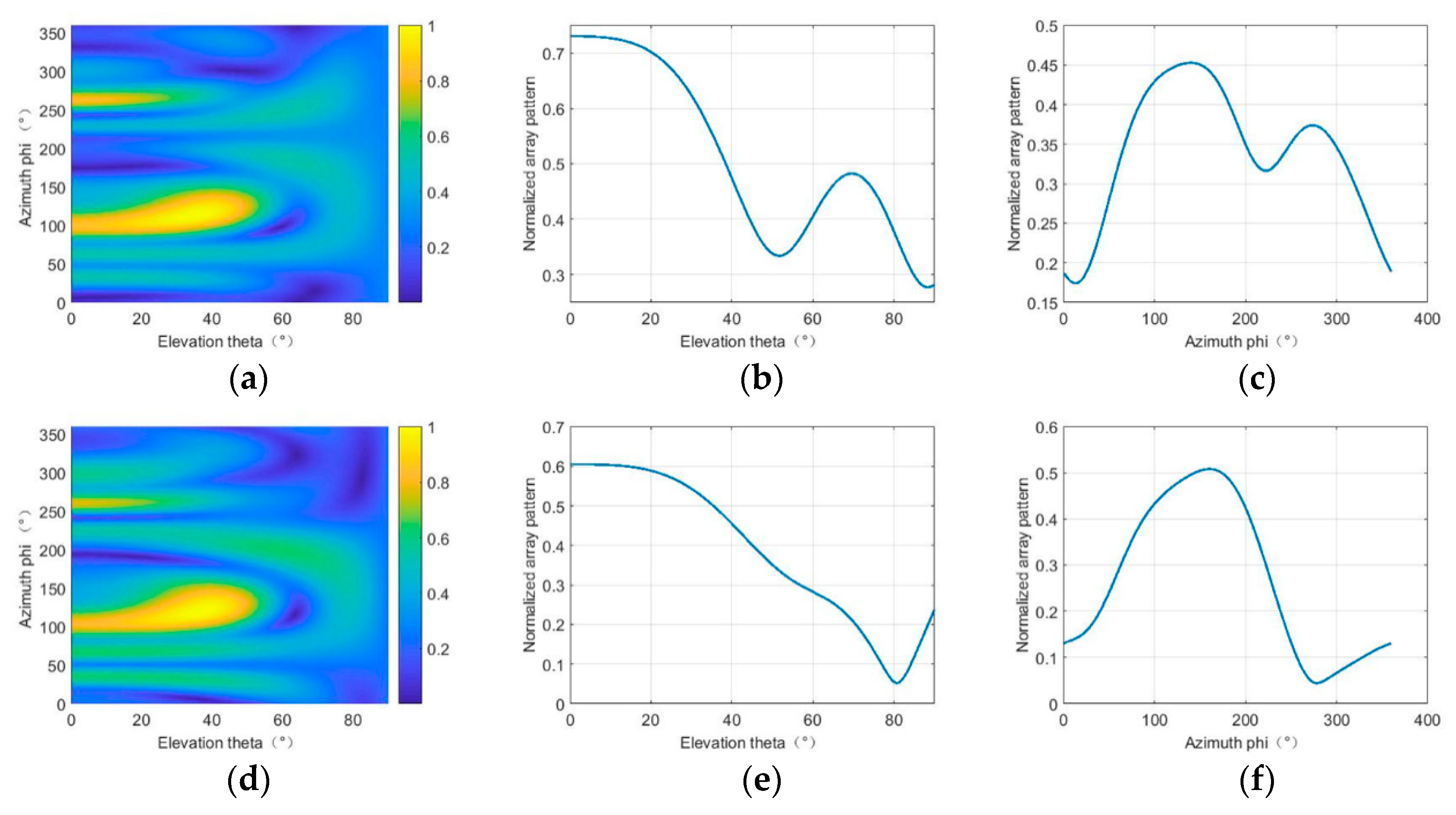
3.1. Basic Beamforming Performance of L-Array

The purpose of the beamformer is to maximize the antenna beam gain towards the desired direction. It is achieved by combining the signals of the different antenna elements with a proper phase shift. The basic beamforming method is to sum the sampling signals of the receiving channels after a phase compensation. In practice, this kind of phase compensation is usually carried out in the way of digital beamforming (DBF). For the L-array employed in this paper, it can be expressed as Equation (2).

$$\{\begin{array}{l}E(\theta ,\phi )=E_x(\theta ,\phi )+E_y(\theta ,\phi )\\ E_x(\theta ,\phi )={\displaystyle \sum _{n=1}^{N_x}{I}_{x_n}{e}^{-j2n\pi d_x(\sin \phi \cos \theta -\sin {\phi }_0\cos {\theta }_0)}}\\ E_y(\theta ,\phi )={\displaystyle \sum _{n=1}^{N_y}{I}_{y_n}{e}^{-j2n\pi d_y(\cos \phi \cos \theta -\cos {\phi }_0\cos {\theta }_0)}}\end{array}$$

(2)

where $E(\theta ,\phi )$, $E_x(\theta ,\phi )$, $E_{\mathrm{y}}(\theta ,\phi )$ represents the sampled values of the electric field strength of the entire array, the x-axis and y-axis’s subarrays. $N_x=N_y=3$, the number of antenna element on the two baselines. $I_{x_n}$ and $I_{y_n}$ are the complex sampling amplitudes of the elements distributed along the x-axis and y-axis. $({\theta }_0,{\phi }_0)$ is the basis of phase compensation, which is also the target direction of the beamforming. Naturally, $E(\theta ,\phi )$ has the maximum value only when Equation (3) holds. Since the L-array has a 2-D structure, Equation (3) has a unique solution that enables the specific pointing at both azimuth and elevation. Unlike linear arrays, this will not cause coning ambiguity or grating lobes [19]. Once the array and the pointing direction is fixed, $E(\theta ,\phi )$ is only determined by the incident direction $(\theta ,\phi )$ of the signal, thus it is also called the array radiation pattern. It is apparent that the basic performance of the array radiation pattern is mainly determined by the number of antennas and space between adjacent elements [20,21].

$$\{\begin{array}{l}\cos \phi \cos \theta =\cos {\phi }_0\cos {\theta }_0\\ \sin \phi \cos \theta =\sin {\phi }_0\cos {\theta }_0\end{array}\Rightarrow \{\begin{array}{l}\phi ={\phi }_0\\ \theta ={\theta }_0\end{array}$$

(3)

The computed radiation pattern of the whole array is shown in Figure 5. The direction of the beamforming pointing is $\phi ={113}^{\circ },\theta ={35}^{\circ }$, which is the transmitting and incident direction of the oblique backscatter echoes. Figure 5a is the normalized array pattern at the frequency point of 5 MHz. Figure 5b,c are the sections of $\phi ={113}^{\circ },\theta ={35}^{\circ }$, respectively. Figure 5d–f and Figure 5g–i, respectively, are the corresponding simulation results of 10 MHz and 15 MHz. With the increase of the frequency and the relative aperture of the antenna array, the beamwidth also decreases gradually, which means better directivity. In azimuth, the beam width of the three representative frequencies are 128°, 74° and 50° respectively. In the low-frequency band, such a miniaturized L-array is indeed difficult to form a very narrow beam. But in practice, even if the operating frequency is 5 MHz, it has formed an effective spatial filtering for interference signals from the other two-thirds directions. In addition, in the 360 ° azimuth range, except in the specified direction, there are no other grating lobes generated, which is not available for general linear array. In elevation, although the directivity is not as good as in azimuth, it has a good weakening ability for high elevation signals. The advantage of this is that the vertical echoes generated by the upward sidelobe of the transmitting antenna will be suppressed. In addition, the influence on the interpretation of the oblique backscatter signals will be reduced. In Cui’s research, the 2-hop vertical echoes have a great interference on the extraction of the oblique backscatter signals [17].

3.2. The Weight Vector of Beamforming

In essence, it can be understood that the essence of beamforming is to obtain a better output by weighting and summing the antennas’ signal. Once $E(\theta ,\phi )$ is rewritten as Equation (4), the weights can be considered as the phase compensations required in the beamforming.

$$\begin{array}{c}E(\theta ,\phi )={\displaystyle \sum _{n=1}^{N_x}{I}_{x_n}{e}^{-j2n\pi d_x(\sin \phi \cos \theta )/\lambda }}{e}^{j2n\pi d_x\sin {\phi }_0\cos {\theta }_0/\lambda }+{\displaystyle \sum _{n=N_x+1}^{N_x+N_y}{I}_{y_n}{e}^{-j2(n-N_x)\pi d_y(\cos \phi \cos \theta )/\lambda }}{e}^{j2(n-N_x)\pi d_y\cos {\phi }_0\cos {\theta }_0/\lambda }\\ \begin{array}{l}=w^{H}s={\displaystyle \sum _{n=1}^{N_x+N_y}{w}_n^{*}{s}_n}\\ w={[w_1,w_2,\cdots w_n]}^T,w_n=\{\begin{array}{l}{e}^{j2n\pi d_x{\sin }_0\cos {\theta }_0/\lambda },1\le n\le N_x\\ e^{j2(n-N_x)\pi d_y\cos {\phi }_0\cos {\theta }_0/\lambda },N_x<n\le N_x+N_y\end{array}\\ s={[s_1,s_2,\cdots s_n]}^T,s_n=\{\begin{array}{l}{I}_{x_n}{e}^{-j2n\pi d_x\sin \phi \cos \theta /\lambda },1\le n\le N_x\\ I_{y_n}{e}^{-j2(n-N_x)\pi d_y\cos \phi \cos \theta /\lambda },N_x<n\le N_x+N_y\end{array}\end{array}\end{array}$$

(4)

where $H$ indicates the conjugate transposition, $*$ represents the complex conjugation and $T$ is the transpose symbol. $I$ represents the integrated signal arriving at the antenna. The signal sequence and the weight vector are $w$ and S respectively.

If there are N snapshots of the signal, the output of the beamformer for time $t$ can be expressed as $y(t)$ in Equation (5).

$$y(t)=w^{H}s(t),t=1,2,\cdots ,N$$

(5)

For a particular signal sequence $d(t)$ of the incident direction of $({\theta }_d,{\phi }_d)$, reference to Equation (1), $s(t)$ can be expressed as Equation (6).

$$s(t)=a({\theta }_d,{\phi }_d)d(t)$$

(6)

Thus, the average power can be expressed as Equation (7).

$$P(w)=E[{\left|y(t)\right|}^2]=w^{H}E[s(t)s^H(t)]w=w^{H}Rw=E[{\left|d(t)\right|}^2]{\left|w^{H}a({\theta }_d,{\phi }_d)\right|}^2$$

(7)

where $E[•]$ indicates the expectation, and $R$ is the autocorrelation matrix of the echo signals of the array.

Combining Equations (1) and (4), Equation (8) can be obtained. It is clear that in the ideal situation without interference signal and noise, the maximal output of the array is $N_x+N_y$ times compared with a single antenna. $w$ is the optimal weight vector of the beamforming.

$${\left|w^{H}a({\theta }_d,{\phi }_d)\right|}^2=N_x+N_y$$

(8)

However, when there are noises and interference signals from other directions, $s(t)$ and $P(w)$ should be rewritten into Equations (9) and (10).

$$\begin{array}{l}s(t)=[a({\theta }_d,{\phi }_d),a({\theta }_{i_1},{\phi }_{i_1}),\cdots ,a({\theta }_{i_J},{\phi }_{i_J})]\left[\begin{array}{c}d(t)\\ i_1(t)\\ ⋮\\ i_J(t)\end{array}\right]+\left[\begin{array}{c}{n}_0(t)\\ n_1(t)\\ ⋮\\ n_J(t)\end{array}\right]\\ I(t)=d(t)+i_1(t)+\cdots +i_J(t)+n_0(t)+n_1(t)+\cdots +n_J(t)\end{array}$$

(9)

$$P(w)=E[{\left|d(t)\right|}^2]{\left|w^{H}a({\theta }_d,{\phi }_d)\right|}^2+{\displaystyle \sum _{k=1}^{J}E[{\left|i_k(t)\right|}^2]{\left|w^{H}a({\theta }_{i_k},{\phi }_{i_k})\right|}^2}+{\Vert w\Vert }^2{\displaystyle \sum _{k=1}^J{\Vert n_k(t)\Vert }^2}$$

(10)

where $i_k(t)$ is the kth interference signal with the incident direction of $({\theta }_{i_k},{\phi }_{i_k})$. The corresponding array manifold is $a({\theta }_{i_k},{\phi }_{i_k})$. $J$ is the number of interference signals. In addition, $\Vert •\Vert$ represents the norm.

In this case, the weight vector $w$ is no longer optimal. Although the power of the desired signal is still maintained, due to the interaction of interference signals and noises, the output of the whole array may not have the best signal to interference noise ratio (SINR). For the large arrays, this problem is not serious. A large number of array elements will make the main beam very narrow. After ultra-low sidelobe processing, with a limited broadening of the main lobe, a quite low sidelobe level can also be obtained [21], which can effectively suppress the interference. However, for the miniaturized array, this may have a greater impact on the detection. Especially for the oblique backscatter sounding of the ionosphere, the weak signals may be submerged in the complex interferences of the HF band. Basic beamforming may not achieve the ideal results.

3.3. Adaptive Beamforming

In order to make the array get better beamforming effect according to the actual signal environment, many adaptive digital beamforming (ADBF) algorithms have been developed and widely used [22,23,24]. By adaptively adjusting the weight vector according to the signal environment, ADBF can perform better spatial filtering to enhance the desired signal and suppress interference. Among them, the sampling matrix inversion (SMI) beamformer [25] and the Eigenspace-based beamforming (ESB) algorithm are two typical adaptive beamforming methods [26]. However, the application effect on the miniaturized L-array is rarely reported.

3.3.1. The Sampling Matrix Inversion Beamformer

The basic idea of the SMI algorithm is to minimize the total output power of the entire array while keeping the signal energy in the desired direction constant. It is an optimal beamformer under the linear constrained minimum variance criterion. SMI beamformer sets the constraint conditions of weight vector as Equation (11).

$$\underset{w}{\min }E[\left|y{(t)}^2\right|]=\underset{w}{\min }\left\{w^{H}Rw\right\},s.t.w^{H}a({\theta }_d,{\phi }_d)=1$$

(11)

For this constraint problem, the weight vector can be solved by Lagrange multiplier method. When Equation (12) is defined as the objective function, the solution of the optimal weight vector $w_{opt}$ can be expressed as Equation (13) [27].

$$L(w)=w^{H}Rw+{\lambda }^{’}[w^{H}a({\theta }_d,{\phi }_d)-1]$$

(12)

$$w_{opt}=\mu R^{-1}a({\theta }_d,{\phi }_d),\mu =\frac{1}{a^H({\theta }_d,{\phi }_d)R^{-1}a({\theta }_d,{\phi }_d)}$$

(13)

In order to investigate the application effect of SMI algorithm on the miniaturized L-array, a simulation experiment was carried out. Under the condition that an interference signal with the same power level as the desired signal comes from $\phi ={270}^{\circ }$, $\theta ={80}^{\circ }$, a random azimuth with an elevation that approximates the vertical sounding echoes. The signal-to-noise ratio (SNR) is set at 5 dB. The simulation results employing SMI beamformer at the frequency point of 15MHz can be shown as Figure 6.

Employing the SMI beamformer, the intensity of the desired signal is also effectively maintained, and the maximum gain point of the pattern is still at $\phi ={113}^{\circ },\theta ={35}^{\circ }$. Different from the conventional beamforming, there is a deep zero depression at the incident direction of the interference signal. In elevation, at $\theta ={80}^{\circ }$, the normalized level of pattern decreases from 0.377 to 0.055. The influence of the vertical sounding signals and its 2-hop echoes caused by the side lobe of the transmitting antenna can be reduced greatly. In an ideal case, if the 2-hop vertical echoes are considered to be suppressed below the level of the oblique backscatter signals, then the low frequency part of the oblique backscatter ionogram do not have to be deducted in the inversion process, which is actually expanding sounding cover range [28]. In azimuth, at $\phi ={270}^{\circ }$, the normalized level drops from 0.373 to 0.053. The interference signals from this direction can be effectively suppressed without affecting the extraction of the desired signals. The simulation results show that the SMI algorithm is still applicable to the miniaturized L-array, with an ideal spatial filtering effect.

3.3.2. Eigenspace-Based Beamformer

Eigenspace-based beamforming (ESB) algorithm can be regard as an improvement of SMI. Assuming that there is one desired signal but with $J$ interferences (which is generally assumed that $J<N_x+N_y$), the eigenvalue decomposition of the covariance matrix $R$ with infinite sampling points can be computed as Equation (14).

$$R={\displaystyle \sum _{i=1}^{J+1}{\lambda }_i{u}_i{u}_i^H+{\sigma }_n^2{\displaystyle \sum _{i=J+2}^{N_x+N_y}{u}_i{u}_i^H}}$$

(14)

where ${\lambda }_1\ge {\lambda }_2\ge \cdots {\lambda }_{J+1}>{\lambda }_{J+2}=\cdots ={\lambda }_{N_x+N_y}={\sigma }_n^2$ are the $N_x+N_y$ eigenvalues, $u_i(i=1,2,\cdots ,N_x+N_y)$ are the corresponding eigenvectors. Then, in SMI, the optimal weight vector $w_{opt}$ can be rewritten as Equation (15):

$$w_{opt}=\mu E_s{D}_s^{-1}{E}_s^{H}a({\theta }_d,{\phi }_d)+\mu E_n{D}_n^{-1}{E}_n^{H}a({\theta }_d,{\phi }_d)$$

(15)

where $D_s=diag({\lambda }_1,\cdots ,{\lambda }_{J+1})$, $D_n=diag({\lambda }_{J+2},\cdots ,{\lambda }_{N_x+N_y})$. $E_s=[u_1,\cdots ,u_{J+1}]$ and $E_n=[u_{J+2},\cdots ,u_{N_x+N_y}]$ constitute the signal subspace and noise subspace respectively. Under the ideal condition, Equation (16) should be established [29]. Thus, the weight vector $w_{opt}=w_0=\mu E_s{D}_s^{-1}{E}_s^{H}a({\theta }_d,{\phi }_d)$ should only have the signal subspace component.

$$E_n^{H}a({\theta }_d,{\phi }_d)=0$$

(16)

However, considering the actual situation, the number of snapshots is limited. The signal will leak into the noise subspace. Thus, Equation (16) is no longer established, which will lead to the decline of the output SINR and may cause the pattern distortion [30]. This phenomenon is more serious in the case of high SNR.

An improved method proposed by Yu J. L. et al. is to discard the components of the weight vector in the noise subspace. That is, the weight vector is projected to the signal subspace. Then the weight vector can be rewritten as Equation (17). As the weight vector is located in the signal subspace, the weakening of the signal caused by signal subspace leakage of SMI algorithm can be significantly reduced [31].

$$w_1=\mu E_s{D}_s^{-1}{E}_s^{H}a({\theta }_d,{\phi }_d)=E_s{E}_s^H{w}_0$$

(17)

Figure 7 shows the simulation results of SMI and ESB beamformer when the SNR is adjusted to 15dB. Figure 7a is the array pattern of SMI beamformer, Figure 7b,c respectively show the sections of $\phi ={113}^{\circ }$ and $\theta ={35}^{\circ }$. In the case of high SNR, the SMI pattern is distorted and the beam pointing is deflected. As shown in Figure 7b,c, the array gain of the desired direction is weakened and another high sidelobe is generated. In contrast, the array pattern of ESB beamformer shown in Figure 7d still has a good performance on the L-array. The beam pointing is still correct. In the sections of $\phi ={270}^{\circ }$, $\theta ={80}^{\circ }$ showing in Figure 7e,f, the interference direction forms a deeper depression.

However, the ESB also has its disadvantages. When the desired signal is too weak, discarding the noise subspace will cause a large error. Therefore, ESB has a better performance for stronger desired signal [26]. This is also verified by the processing of actual signals below.

4. Beamforming of the Oblique Backscatter Ionogram

To obtain ionospheric information in a large area, the oblique backscatter sounding usually works in a frequency scanning mode. With the sounding waveform modulated by m-sequence encoded by pseudo-random two-phase code, the detection is whole coherent. Thus, at every frequency, multiple coherent accumulations are often carried out to improve the SNR. If a signal detection includes $M$ frequency points, $K$ coherent accumulations are carried out on each frequency, the sampling echo signal sequence can be expressed:

$$\left[s_{i,f_m,k}(t_1),s_{i,f_m,k}(t_2),\cdots ,s_{i,f_m,k}(t_N)\right]$$

(18)

where N is the length of the m-sequence, which is also the total number of sounding range gates. Then $t_1,t_2,\cdots ,t_N$ represent the sampling moment and also represent the distance gate of the echo. $i,f_m,k$ represent the sequence number of channel, frequency and coherent accumulation respectively.

After the cross-correlation with m-sequence $\left(t_1,t_2,\cdots ,t_N\right)$, the pulse compressed signal sequence can be obtained as Equation (19).

$$\left[S_{i,f_m,k}(t_1),S_{i,f_m,k}(t_2),\cdots ,S_{i,f_m,k}(t_N)\right]=\left[s_{i,f_m,k}(t_1),s_{i,f_m,k}(t_2),\cdots ,s_{i,f_m,k}(t_N)\right]\left(\begin{array}{cccc}{m}_1& m_N& \cdots & m_2\\ m_2& m_1& \cdots & m_3\\ ⋮& ⋮& \ddots & ⋮\\ m_N& m_{N-1}& \cdots & m_1\end{array}\right)$$

(19)

Hence, on any range gate $t_n$, the covariance matrix of the sampling sequence can be obtained after $K$ times coherent sounding as Equation (20).

$$R=\left[\begin{array}{cccc}{S}_{1,f_m,1}(t_n)& S_{1,f_m,2}(t_n)& \cdots & S_{1,f_m,K}(t_n)\\ S_{2,f_m,1}(t_n)& S_{2,f_m,2}(t_n)& \cdots & S_{2,f_m,K}(t_n)\\ ⋮& ⋮& \ddots & ⋮\\ S_{I,f_m,1}(t_n)& S_{I,f_m,2}(t_n)& \cdots & S_{I,f_m,K}(t_n)\end{array}\right]{\left[\begin{array}{cccc}{S}_{1,f_m,1}(t_n)& S_{1,f_m,2}(t_n)& \cdots & S_{1,f_m,K}(t_n)\\ S_{2,f_m,1}(t_n)& S_{2,f_m,2}(t_n)& \cdots & S_{2,f_m,K}(t_n)\\ ⋮& ⋮& \ddots & ⋮\\ S_{I,f_m,1}(t_n)& S_{I,f_m,2}(t_n)& \cdots & S_{I,f_m,K}(t_n)\end{array}\right]}^H$$

(20)

Based on the covariance matrix $R$, the weight vector can be determined employing an SMI or ESB beamformer:

$$\left[w_{1,f_m}(t_n),w_{2,f_m}(t_n),\cdots ,w_{I,f_m}(t_n)\right]$$

(21)

Therefore, the signal after beamforming can be expressed as a form of weighted summation of the signals of the channels:

$$S_{f_m,k}(t_n)=\left[w_{1,f_m}(t_n),w_{2,f_m}(t_n),\cdots ,w_{I,f_m}(t_n)\right]{\left[S_{1,f_m,k}(t_n),S_{2,f_m,k}(t_n),\cdots ,S_{I,f_m,k}(t_n)\right]}^T$$

(22)

After k-times coherent accumulation, the amplitude sequence of the signal for the frequency point $f_m$ at $t_n$ can be obtained as Equation (23).

$$A_{f_m}(t_n)=\left|{\displaystyle \sum _{k=1}^K{S}_{f_m,k}(t_n)}\right|=\left|{\displaystyle \sum _{k=1}^K\left\{\left[w_{1,f_m}(t_n),w_{2,f_m}(t_n),\cdots ,w_{I,f_m}(t_n)\right]{\left[S_{1,f_m,k}(t_n),S_{2,f_m,k}(t_n),\cdots ,S_{I,f_m,k}(t_n)\right]}^T\right\}}\right|$$

(23)

Since the weight vector is independent of the coherence number, the order of weighting and summation can be interchanged as Equation (24). In this way, the number of multiplication operations can be reduced, especially when the number of coherent accumulations is large.

$$A_{f_m}(t_n)=\left|{\displaystyle \sum _{k=1}^K{S}_{f_m,k}(t_n)}\right|=\left|\left[w_{1,f_m}(t_n),w_{2,f_m}(t_n),\cdots ,w_{I,f_m}(t_n)\right]{\displaystyle \sum _{k=1}^K{\left[S_{1,f_m,k}(t_n),S_{2,f_m,k}(t_n),\cdots ,S_{I,f_m,k}(t_n)\right]}^T}\right|$$

(24)

So that, for the frequency point $f_m$, the amplitude sequence on the oblique backscatter ionogram diagram along the range gates can be expressed as Equation (25).

$$A_{f_m}={\left[A_{f_m}(t_1),A_{f_m}(t_2),\cdots ,A_{f_m}(t_N)\right]}^T$$

(25)

As a result, the whole oblique backscatter ionogram of $M$ frequencies can be finally computed as Equation (26).

$$A=\left[A_{f_1},A_{f_2},\cdots ,A_{f_M}\right]$$

(26)

5. Experiments and Results

In order to verify the practical application effect on the ionospheric oblique backscatter sounding of the system with the miniaturized L-shaped antenna array proposed in this paper, a verification experiment was carried out on 14 January 2019 at Xiantao, in Hubei province, China. As shown in Figure 8, the experiment adopts the mode of off-site to avoid the near-field interference caused by continuous wave transmitting. The transmitting subsystem was set at Wuhan (114.48°E, 30.50°N), and the multi-channel receiver and antenna array are placed at Xiantao (113.50°E, 30.17°N). The distance between the two places is about 89.32 km. The transmitting antenna points to 113° in azimuth. As the oblique backscatter sounding has a large coverage, on the far-field condition, the transmitting and receiving subsystem can be approximated as the same address. The sounding adopts the continuous wave modulated by a 511-bit pseudo-random two-phase m-sequence, with a transmitting power of 500 W. The bit-width is 25.6 μs and the corresponding distance resolution is 3.84 km. The operating frequency band is selected in 5–15 MHz, with a sweeping step of 0.2 MHz. The number of coherent accumulations is 256.

5.1. Basic Function Verification

Figure 9 shows the original swept- frequency oblique backscatter ionograms of six channels. Although the transmitting power is only 500 W, under the effect of the pulse compression gain of m-sequence and multiple coherent accumulation, this system conducted the ionospheric oblique backscatter sounding. The signals between 260 and 300 km are the vertical reflected echoes. The oblique backscatter echoes appeared from 520 to 900 km. It is obvious that the power of vertical echoes is much stronger than that of oblique backscatter echoes. In the vertical echo part, the SNR generally larger than 220 dB, while for the oblique backscatter part, it is difficult to reach 160 dB. The strongest oblique backscatter signals are mainly distributed in the low frequency part, which is most likely due to the superposition of the 2-hops of the vertical-incidence echoes. As shown in Figure 9, the highest reflection frequency of the vertical-incidence signal is 6.2 MHz. This means that it is difficult to judge the mode of the echo signals below 600 km and 6.2 MHz. In essence, it limits the effective range and the operating frequency band of the oblique backscatter sounding.

Moreover, in addition to the desired signal, for the system operating in the HF band, there are also many strong radio-frequency (RF) interferences entering the receiver simultaneously. Sometimes the intensity of these interference signals can be quite large. At 6 MHz, 9.4 and 9.8 MHz, as examples, the SNR of the interference signals even exceed 205 dB, completely submerging the useful signals, which will also cause great difficulties in the extraction of oblique backscatter leading trace.

5.2. Conventional Beamforming of Oblique Backscatter Ionogram

The comparison between the results of the oblique backscatter ionograms obtained by directly sum the signals of the six channels’ and the conventional DBF can be shown in Figure 10, with Channel 1 as a reference. In the lower frequency band, in the vertical echoes’ regions, the directly summed ionogram has the best SNR. At 5.2 MHz, 268.8 km as an example, the SNR of Channel 1 is 236.1 dB, the SNRs of the directly summed ionogram and the DBF result are 240.6 dB and 214.4 dB, respectively. This means that for the vertical echo signals, which are close to the vertical incidence, summing the six channels directly can enhance the signal strength, while DBF weakens it. It reflects the spatial filtering effect of DBF. But in the high frequency band, at 7 MHz, 691.2 km for example, with only oblique backscatter signal, the SNR of Channel 1, the directly summed ionogram and DBF result are 181.1 dB, 160.5 dB and 177.2 dB. Obviously, there is destructive interference in the way of directly summing while DBF retains the desired signal. Refer to Channel 1, it seems that DBF also weaken the SNR. This is because that under the effect of the spatial filtering, DBF not only retains the desired signal, but also suppresses the signals from other directions, resulting in a decrease of the total power.

For further explanation, Figure 11 and Figure 12 extract the signals of 5.2 MHz and 7 MHz respectively normalizing the SNR as examples to compare. At 5.2 MHz, the vertical echo is the strongest signal with a relatively strong 2-hop. For the three processing methods, the average background noise is −110.9 dB, −116 dB and −97.77 dB, respectively. The SNR of DBF’s vertical echo is the lowest, which means that the vertical incidence signal is suppressed. However, at 7 MHz, the signal processed by DBF has the best normalized SNR and the steepest leading edge, the average background noise is −85.54dB. And since the incident direction is no longer vertical to the plane of the antenna array, the destructive interference is generated by the direct addition of the multi-channel signals, with the worst background noise of −62.9 dB. The average background noise of Channel 1 is −76.6 dB, in the middle.

For the frequency points with RF interference signals, DBF also shows a certain suppression effect. Taking 6 MHz as an example, the signals of Channel 1, directly summing and DBF can be extracted as Figure 13. Comparing with Channel 1 and the directly summing method, the average background noise level is significantly reduced after DBF. For the area between vertical echo and oblique backscatter echoes, from about 300 km to 580 km, the interference signals are suppressed. Although this effect seems to be limited, it still means a steeper leading edge which would be easier to extract.

5.3. Adaptive Beamforming of Oblique Backscatter Ionogram

Figure 14 show the oblique backscatter ionograms processed by the SMI and ESB adaptive beamforming algorithms. To truly reflect the suppression effect of vertical echoes and interference signals, Channel 1 is still taken as the reference in this section. Obviously, the adaptive beamformers greatly weaken the vertical echo signals much better than conventional DBF as Figure 10c. It is also reasonable to believe that the 2-hop echoes will not interfere with the oblique backscatter signals. Therefore, in the whole frequency band of 5–9.2 MHz, the signals over 520 km can be traced and extracted as the oblique backscatter echoes. It is equivalent to extending the sounding range towards the transmitting station.

For typical RF interference signals, such as 6 MHz, 9.4 MHz and 9.8 MHz, compared with the conventional DBF, the adaptive beamformers have much better suppression effects as shown in Figure 14b,c. Especially for ESB algorithm, some strong interference signals such as 9.4 MHz and 12.2 MHz are almost completely filtered out.

It is undeniable that both SMI and ESB seem to reduce the SNRs. When the adaptive beamformers suppress the vertical signals in the low frequency band greatly, the SNRs of the higher frequencies are not improved. This is because that whether it is SMI or ESB, the basic idea is to keep the desired signals while minimizing the output power of the whole array. This makes the total output power of the array decrease when the desired signal or interference exist. But when there is no desired or interference signals, the noise power cannot be reduced equally. And due to the effect of the spatial filtering, echo signals from other azimuths caused by the side lobe of the transmitting antenna are also weakened substantially together. In contrast, the effect of this signal processing method for obtaining the leading edges of the desired pointing direction should be more meaningful.

In order to better show the application effect of adaptive beamforming in the oblique backscatter sounding, some of the specific typical frequencies, such as 5.2 MHz with strong vertical signal, 6 MHz with great interference, 7 MHz with a strong desired signal and 8.8 MHz with a weak one, have been extracted as Figure 15, Figure 16, Figure 17 and Figure 18.

For 5.2 MHz, in Figure 15a, it is obvious that the 2-hop of the vertical echo signal of channel 1 is a pseudo leading and can easily be mistaken for the desired echo signal. But through the adaptive beamforming, the vertical incident signals are well suppressed. If the same attenuation coefficient (24dB) of the 2-hop echo signal in Figure 15a is referred, the 2-hop signals in Figure 15b,c are limited near the background noise level and will not affect the discrimination of the leading edge. Therefore, while it seems that the SNR in Figure 15a looks better, in fact, Figure 15b,c are more accurate.

As for the strong interference signal at 6 MHz. From Figure 16a, it can be seen that the strength of the interference signal almost equal to the 2-hop of the vertical echo signal. At the group distance of 583.7 km, the strength of the signal is only 23.57 dB higher than the average background level. While in Figure 16b,c, this value can reach 45.69 dB and 44.85 dB. For the area from 300 km to 580 km, the suppression ability of interference signal is even better than DBF as Figure 13c. Especially for the SMI algorithm, Figure 16b shows a very clear and steep leading edge. Although the SNRs of Figure 16b,c are not as good as Figure 16a relative to the strongest signal, relaying on the adaptive beamforming techniques, the interference signal is greatly suppressed, while the desired signal is still maintained.

Figure 17 and Figure 18 demonstrate the performance of two adaptive beamforming algorithms when the desired signal is stronger and weaker, respectively. For a strong desired signal of 7 MHz, in Figure 17, as described in the above simulation results, the performance of SMI is poorer, and the leading edge of the oblique backscatter signal is not as steep as ESB and channel 1′s. But when the desired signal is weaker, at 8.8 MHz, for example, SMI beamformer not only has a lower and more stable background noise level than channel 1, but also sharpens the echo leading edge which is much easier to be extracted. Meanwhile, ESB beamformer has a good processing effect for both 7 MHz and 8.8 MHz. But in Figure 18c, the processing effect of ESB for strong signal seems better. For channel 1, the signal at 937 km is only 2 dB stronger than that at 837 km, but with ESB algorithm, the difference is increased to be 15.4 dB, and while the strongest point in Figure 18b is still at 837 km.

Figure 19 shows the oblique backscatter ionogram processed by the Constant False-Alarm Rate (CFAR) processor. Although the SNRs are less in ionograms with SMI and ESB, the contrast between the oblique backscatter signals and the background is improved obviously. Compared with single channel reception and conventional beamforming, the vertical echo signal after adaptive beamforming can be approximately ignored. The interference problem of 2-hop signals of the vertical echoes with linear array is also well solved [17]. And for the oblique backscatter ionogram of channel 1 in Figure 19a, due to the strong interference of some frequency points, after CFAR processing, the useful signals are also eliminated at the same time, which results in some discontinuous points along the leading-edge trace, such as at 5.8 MHz, 6 MHz and so on. A similar situation also appears in the oblique backscatter ionogram of conventional DBF as Figure 19b. For the ESB’s ionogram, which is shown in Figure 19d, the signal can be clearly identified above 7 MHz, but below 7 MHz, the trace is not as clear as the ionogram processed by the SMI beamformer in Figure 19c. From 5 MHz to 9.2 MHz, the SMI ionogram has a continuous leading trace. Especially below 6MHz, although the desired signals are rather weak, the SMI beamformer still makes a continuous and clear trace. This is also the main purpose of the various processing for the oblique backscatter ionograms. Then from a comprehensive point of view, although ESB has better performance for stronger signals, SMI is a more suitable adaptive beamforming processing method for the low power system and the miniaturized L-shaped antenna array described in this paper.

6. Conclusions

In this paper, a dedicated multi-channel oblique backscatter sounder with a miniaturized L-shaped receiving antenna array was developed. Relaying on the high pulse compression gain of m-sequence, a transmission power of 500 W can guarantee the sounding performance. The simulation analysis and experimental results verify that the L-shaped antenna array can achieve a good 2-D beam pointing at elevation and azimuth simultaneously. By using the adaptive beamforming technique, the directional reception of the signal is more optimized, which not only weakens the influence of the two-hop ionospheric vertical echoes on the low-frequency band, but also suppressing the other RF interferences. Thus, on the ionograms, the oblique backscatter echo signals are enhanced and the contrast of the whole ionogram is remarkably improved. Through the analysis of some frequency signal sequences, it can be found that the adaptive beamformers makes the trace leading edge easier to be identified and extracted in the inversion process. Finally, by comparing the results of CFAR and de-noising, it can be concluded that SMI beamformer is more suitable for the low power system and the miniaturized L-shaped antenna array described in this paper.

From the practice of this paper, it can be seen that employing 2-D antenna array to conduct the ionospheric oblique backscatter sounding has considerable research and application value. Typical arrays and processing algorithms are used in the current work. Naturally, how to further combine the characteristics of the ionosphere to study and design the optimal array structure and processing method should be the research goal of the next stage. Some existing related theories may be used for reference. But this still requires further experiments and analysis of the observational data.

References

1. Croft, T.A. Sky-wave backscatter: A means for observing our environment at great distances. Rev. Geophys. 1972, 10, 73–155. [Google Scholar] [CrossRef]
2. Raab, F.H.; Caverly, R.; Campbell, R.; Eron, M.; Hecht, J.B.; Mediano, A.; Myer, D.P.; Walker, J.L.B. HF, VHF, and UHF systems and technology. IEEE Trans. Microw. Theory Tech. 2002, 50, 888–899. [Google Scholar] [CrossRef]
3. Headrick, J.M.; Thomason, J.F. Applications of high frequency radar. Radio Sci. 1998, 33, 1045–1054. [Google Scholar] [CrossRef]
4. Settimi, A.; Pezzopane, M.; Pietrella, M.; Bianchi, C.; Scotto, C.; Zuccheretti, E. Testing the IONORT-ISP system: A comparison between synthesized and measured oblique ionograms. Radio Sci. 2013, 48, 167–179. [Google Scholar] [CrossRef]
5. Goodman, J.; Ballard, J.; Sharp, E. A long-term investigation of the HF communication channel over middleand high-latitude paths. Radio Sci. 1997, 32, 1705–1715. [Google Scholar] [CrossRef]
6. Earl, G.F.; Ward, B.D. The frequency management system of the Jindalee over-the-horizon backscatter HF radar. Radio Sci. 1987, 22, 275–291. [Google Scholar] [CrossRef]
7. Occhipinti, G.; Dorey, P.; Farges, T.; Lognonne, P. Nostradamus: The radar that wanted to be a seismometer. Geophys. Res. Lett. 2010, 37, 1480–1493. [Google Scholar] [CrossRef]
8. Lester, M.; Chapman, P.J.; Cowley, S.W.H.; Crooks, S.J.; Davies, J.A.; Hamadyk, P.; McWilliams, K.A.; Milan, S.E.; Parsons, M.J.; Payne, D.B.; et al. Stereo CUTLASS—A new capability for the SuperDARN HF radars. Ann. Geophys. 2004, 22, 459–473. [Google Scholar] [CrossRef] [Green Version]
9. Barry, G.H. A low-power vertical-incidence ionosonde. IEEE Trans. Geosci. Electron. 2007, 9, 86–89. [Google Scholar] [CrossRef]
10. Arthur, P.C.; Cannon, P.S. ROSE: A high performance oblique ionosonde providing new opportunities for ionospheric research. Ann. Geophys. 1994, 37, 135–144. [Google Scholar]
11. Bazin, V.; Molinie, J.P.; Munoz, J.; Dorey, P.; Saillant, S.; Auffray, G.; Rannou, V.; Lesturgie, M. Nostradamus: An OTH Radar. IEEE Aerosp. Electron. Syst. Mag. 2007, 21, 3–11. [Google Scholar] [CrossRef]
12. Cameron, A. The Jindalee operational radar network: Its architecture and surveillance capability. In Proceedings International Radar Conference; IEEE: Perth, Australia, 1995. [Google Scholar]
13. Anderson, S.J. Adaptive remote sensing with HF skywave radar. IEE Proc. F-Radar Signal Process. 1992, 139, 182–192. [Google Scholar] [CrossRef]
14. Greenwald, R.A.; Baker, K.B.; Dudeney, J.R.; Pinnock, M.; Jones, T.B.; Thomas, E.C.; Villain, J.-P.; Cerisier, J.-C.; Senior, C.; Hanuise, C.; et al. DARN/SuperDARN. Space Sci. Rev. 1995, 71, 761–796. [Google Scholar] [CrossRef]
15. Liu, J.H.; Zhao, Z.Y.; Chen, X.T.; Yao, Y.G. The real-time DSP system design of the ionospheric oblique backscattersounding system. J. Wuhan Univ. Nat. Sci. Ed. 2003, 49, 132–136. [Google Scholar]
16. Shi, S.; Yang, G.; Jiang, C.; Zhang, Y.; Zhao, Z. Wuhan Ionospheric Oblique BackscatterSounding System and Its Applications—A Review. Sensors 2017, 17, 1430. [Google Scholar] [CrossRef] [Green Version]
17. Cui, X.; Chen, G.; Wang, J.; Song, H.; Gong, W. Design and Application of Wuhan Ionospheric Oblique BackscatterSounding System with the Addition of an Antenna Array (WIOBSS-AA). Sensors 2016, 16, 887. [Google Scholar] [CrossRef] [Green Version]
18. Chen, G.; Zhao, Z.; Li, S.; Shi, S. WIOBSS: The Chinese low-power digital ionosonde for ionospheric backscatterdetection. Adv. Space Res. 2009, 43, 1343–1348. [Google Scholar] [CrossRef]
19. Fabrizio, G.; Heitmann, A. Single site geolocation method for a linear array. In Proceedings of the 2012 IEEE Radar Conference; Institute of Electrical and Electronics Engineers (IEEE): San Diego, CA, USA, 2012; pp. 885–890. [Google Scholar]
20. Holm, S.; Kristoffersen, K. Analysis of Worst-Case Phase Quantization Sidelobes in Focused Beamforming. IEEE Trans. Ultrason. Ferroelectr. Freq. Control. 1992, 39, 593–599. [Google Scholar] [CrossRef]
21. Hacker, P.; Schrank, H.E. Range distance requirements for measuring low and ultralow sidelobe antenna patterns. IEEE Trans. Antennas Propag. 1982, 30, 956–966. [Google Scholar] [CrossRef]
22. Reed, I.S.; Mallett, J.D.; Brennan, L.E. Rapid Convergence Rate in Adaptive Arrays. IEEE Trans. Aerosp. Electron. Syst. 2007, AES-10, 853–863. [Google Scholar] [CrossRef]
23. Robert, G.L.; Stephen, P.B. Robust minimum variance beamforming. IEEE Trans. Signal Process. 2005, 53, 1684–1696. [Google Scholar]
24. Lee, C.-C.; Lee, J.-H. Eigenspace-based adaptive array beamforming with robust capabilities. IEEE Trans. Antennas Propag. 1998, 45, 1711–1716. [Google Scholar]
25. Parker, D.; Zimmermann, D.C. Phased Arrays-Part 1: Theory and Architectures. IEEE Trans. Microw. Theory Tech. 2002, 50, 678–687. [Google Scholar] [CrossRef]
26. Liao, G.; Zhang, B.; Zhang, L. A New Eigenstructure-Based Algorithm for Adaptive Beamforming. ACTA Electron. Sin. 1998, 26, 22–26. [Google Scholar]
27. Capon, J. High resolution frequency-wavenumber spectrum analysis. Proc. IEEE 1969, 57, 1408–1418. [Google Scholar] [CrossRef] [Green Version]
28. Liu, J.; Liu, W.; Liu, H.; Chen, B.; Xia, X.G.; Dai, F. Average SINR Calculation of a Persymmetric Sample Matrix Inversion Beamformer. IEEE Trans. Signal Process. 2016, 64, 2135–2145. [Google Scholar] [CrossRef]
29. Song, H.; Hu, Y.; Jiang, C.; Zhou, C.; Zhao, Z. Automatic scaling of HF swept-frequency backscatter ionograms. Radio Sci. 2015, 50, 381–392. [Google Scholar] [CrossRef]
30. Dzielski, J.E.; Burkhardt, R.C.; Kotanchek, M.E. Modified MUSIC algorithm for estimating DOA of signals—Comment. Signal Process. 1996, 55, 253–254. [Google Scholar] [CrossRef]
31. Yu, J.L.; Yeh, C.C. Generalized eigenspace-based beamformers. IEEE Trans. Signal Process. 1995, 43, 2453–2461. [Google Scholar]
Figure 1. The specific architecture of the system.
Remotesensing 12 00499 g001
Figure 2. (a) The transmitting channel; (b) the power amplifier; (c) the transmitting antenna.
Remotesensing 12 00499 g002
Figure 3. (a) The overall structure of the receiver; (b) the boards of the analog leading-ends; (c) the photo of the ADC board; (d) the photo of the DDC board.
Remotesensing 12 00499 g003
Figure 4. (a) The layout of the antenna array; (b) the actual scene of the antenna array.
Remotesensing 12 00499 g004
Figure 5. (a) is the normalized array pattern at the frequency point of 5 MHz. (b,c) are the sections of φ = 113 ,   θ = 35 , respectively. (di) are the corresponding simulation results of 10MHz and 15 MHz.
Remotesensing 12 00499 g005
Figure 6. (a) is the top view of Figure 5g, (b,c) are sections of φ = 270 and θ = 80 , respectively. (df) are the corresponding results of using SMI optimal beamformer.
Remotesensing 12 00499 g006
Figure 7. (a) is the array pattern of SMI beamformer, (b,c) respectively show the sections of φ = 113 and θ = 35 . (d) is the array pattern of ESB beamformer, (e,f) show the sections of φ = 270 , θ = 80 .
Remotesensing 12 00499 g007
Figure 8. Map showing the location of the experiment in Wuhan, Xiantao, Hubei province, China and the antenna pointing direction in azimuth.
Remotesensing 12 00499 g008
Figure 9. Oblique backscatter ionograms of six channels.
Remotesensing 12 00499 g009aRemotesensing 12 00499 g009b
Figure 10. (a) The oblique backscatter ionogram of Channel 1; (b) The oblique backscatter ionogram of directly summing; (c) The oblique backscatter ionogram of digital beamforming (DBF).
Remotesensing 12 00499 g010
Figure 11. Normalized signal-to-noise ratio (SNR) of 5.2 MHz; (a) Channel 1; (b) Directly sum; (c) digital beamforming (DBF).
Remotesensing 12 00499 g011
Figure 12. Normalized SNR of 7 MHz; (a) Channel 1; (b) Directly sum; (c) DBF.
Remotesensing 12 00499 g012
Figure 13. Normalized SNR of 6 MHz; (a) Channel 1; (b) Directly summing; (c) DBF.
Remotesensing 12 00499 g013
Figure 14. (a) The oblique backscatter ionogram of Channel 1; (b) The oblique backscatter ionogram of SMI; (c) the oblique backscatter ionogram of ESB.
Remotesensing 12 00499 g014
Figure 15. Normalized SNR of 5.2 MHz; (a) Channel 1; (b) SMI; (c) ESB.
Remotesensing 12 00499 g015
Figure 16. Normalized SNR of 6 MHz; (a) Channel 1; (b) SMI; (c) ESB.
Remotesensing 12 00499 g016
Figure 17. Normalized SNR of 7 MHz; (a) Channel 1; (b) SMI; (c) ESB.
Remotesensing 12 00499 g017
Figure 18. Normalized SNR of 7.8 MHz; (a) Channel 1; (b) SMI; (c) ESB.
Remotesensing 12 00499 g018
Figure 19. The oblique backscatter ionogram after Constant False-Alarm Rate (CFAR) processing and removal of discrete noise; (a) Channel 1; (b) DBF; (c) SMI; (d) ESB.
Remotesensing 12 00499 g019