Abstract
In this paper, we report the results of our work on automated detection of qanat shafts on the Cold War-era CORONA Satellite Imagery. The increasing quantity of air and space-borne imagery available to archaeologists and the advances in computational science have created an emerging interest in automated archaeological detection. Traditional pattern recognition methods proved to have limited applicability for archaeological prospection, for a variety of reasons, including a high rate of false positives. Since 2012, however, a breakthrough has been made in the field of image recognition through deep learning. We have tested the application of deep convolutional neural networks (CNNs) for automated remote sensing detection of archaeological features. Our case study is the qanat systems of the Erbil Plain in the Kurdistan Region of Iraq. The signature of the underground qanat systems on the remote sensing data are the semi-circular openings of their vertical shafts. We choose to focus on qanat shafts because they are promising targets for pattern recognition and because the richness and the extent of the qanat landscapes cannot be properly captured across vast territories without automated techniques. Our project is the first effort to use automated techniques on historic satellite imagery that takes advantage of neither the spectral imagery resolution nor very high (sub-meter) spatial resolution.
1. Introduction
Remote sensing of air-borne and satellite imagery has become a key element of archaeological research and cultural resource management. Combined with field research, remote sensing permits rapid and high-resolution documentation of the ancient landscapes [1,2,3,4]. It also allows for the documentation and monitoring of ancient landscapes that are inaccessible for fieldwork, threatened, or permanently destroyed [5,6,7,8]. The volume and variety of air and space-borne imagery is ever increasing, which is, in theory, of great potential for the field. In practice, however, this “data deluge” is still handled by traditional methods of visual inspection and manual marking of the potential archaeological features. On one hand, researchers cannot handle the quantity of the available data. On the other hand, traditional methods will not do justice to the increasing spectral quality of new data because the researchers use the same method, i.e., a visual judgment based on one’s experience, to all categories of imagery and at best can afford to experiment with a small subset of the spectral information available in the datasets. The only way to address these challenges is to automate some or all tasks in image prospection for archaeological feature detection [9,10,11,12,13,14].
Despite the wide application in domains as diverse as self-driving cars, face recognition, and medical diagnosis, the low success rate of earlier pattern recognition experiments in archaeology has resulted in an overall skepticism in the value of automated object detection for the field [15,16,17,18,19]. As discussed by Cowley [9], some scholars have added to this lack of interest by discouraging the idea of replacing human expert with computer vision in archaeological prospection [2,20]. Such arguments miss the point that the automation of feature extraction is meant to become another tool, and not a replacement, for archaeologists to quickly create a baseline dataset of the features of interest over large geographical areas, especially for studying high-density off-site features with relatively uniform appearance. That is why some have chosen the term semi-automation over automation to emphasize the critical role of human experts in the validation and interpretation of the data [9,10,11,18,21]. The poor results of numerous previous experiments with automated feature detection in archaeology may well lie in the limitations of the traditional pattern recognition methods discussed below. With the advent of deep learning pattern recognition methods, archaeologists can achieve significantly better results; thus, automated feature recognition can now become a standard part of the archaeological remote sensing practice [11,22].
Research on the (semi)-automated detection of manmade landscape objects started in the 1970s [23,24,25,26]. A peak of interest was observed since the 1990s, particularly in urban studies and land use assessment when relatively high resolution (spatial and spectral) satellite imagery became widely accessible [27,28,29,30,31,32,33,34]. Since the mid-2000s, archaeologists have also experimented widely with computational approaches in remote sensing-based archaeological prospection [35,36,37]. The dominant computer vision paradigm in these traditional pattern recognition methods is built on defining explicit prior rules. Based on a combination of the geometric, topographic, and spectral characteristics of the sample features, algorithms are designed to detect similar features in the imagery. In order to improve the outcome, multi-step preprocessing of the imagery and post-processing of the results is necessary [9,10,14,15,16,17,18,19,38,39,40,41,42,43,44,45,46]. For an excellent review of traditional pattern recognition methods applied in archaeology see reference [11].
By necessity, handcrafted algorithms oversimplify the detection task and are unable to come close to human performance for complicated object detection tasks in diverse contexts. In particular, the large number of false positives compared to true positives rendered most of these algorithms of little practical value in archaeological prospection [15,16,17,19,44,45,47]. As discussed by Trier et al. [12], when the true-positive-to-false-positive rate is reasonable, the tasks are so specific that the results cannot be compared with experiments with more varied objects and contexts. The machine learning paradigm in pattern recognition, however, requires no explicit knowledge or prior rules. Rather, the model learns from a sample of positive and negative instances of the objects of interest. Recently, a few experiments have applied nontraditional methods, namely a machine learning random forest algorithm, in archaeological object detection and have outperformed rule-based algorithms [42,48,49,50].
The true paradigm shift in computer vision came about with the advent of neural networks and deep learning [27,51]. In 2012, deep convolutional neural networks (CNNs) dramatically outperformed the best state-of-the-art computer vision models in their speed and accuracy of image classification [52]. CNNs are now used successfully in challenging computer vision tasks such as face detection, self-driving cars, and medical diagnosis [53]. Although deep learning requires large training datasets, transfer learning (or domain adoption), opened the use of pre-trained CNNs to many fields that were restricted by the small size of their training datasets, like archaeology [11,38]. Since 2016, the CNNs have shown a breakthrough in the automation of the archaeological prospection of features with relatively uniform shapes. True positives are notably higher. More importantly, false positives are for the first time low enough to be reasonable to work with [11,12,17,22,47,54]. Furthermore, the models show better tolerance to the variations in the natural and anthropogenic landscape, which opens the scope of their application. In this study, we demonstrate the applicability of CNNs for archaeological prospection by using them to detect the archaeological remains of qanat systems on the Cold War-era CORONA satellite imagery.
A qanat, also known by other names in different countries, is an underground water supply technology composed of horizontal tunnels and a series of vertical shafts [55]. It collects water from an underground water source, usually an aquifer, and transports it underground to the zone of consumption, which might be tens of meters to hundreds of kilometers away from the source (Figure 1 and Figure 2). There is much debate about the origin and the history of diffusion or invention of this water supply technology [56,57,58,59]. What is certain is that by the first centuries of the second millennium CE, rural and urban settlements in a wide range of arid and semi-arid regions of Africa and Asia relied on a variant of the qanat technology to thrive. Therefore, it is important for many archaeological research projects as well as cultural heritage preservation projects in many countries to properly document qanat landscapes.
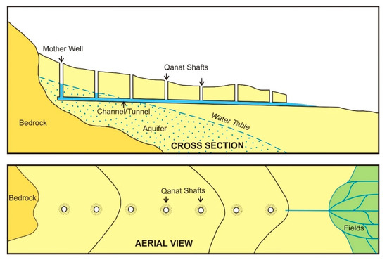
Figure 1.
Schematic diagram of a qanat in mountain or hilly area. Courtesy of Dale Lightfoot.
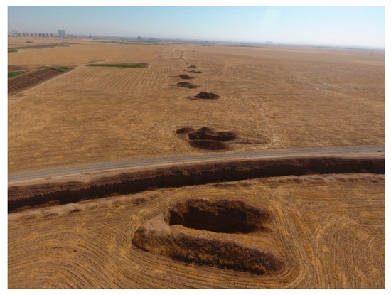
Figure 2.
Alignment of shafts of an abandoned qanat (karez) west of Erbil, near Arab Kandi village.
For the proper mapping of qanat systems, individual shafts that represent the course and complexity of the underground system need to be documented individually (Figure 3). However, mapping qanats at shaft-level is most suitable for small systems and small research areas [60]. Large qanat systems are usually mapped either as a point representing its outlet or as a line representing its approximate path from the source to the outlet. The complexity of qanat systems is inevitably lost when mapping is done only at a high-level identification of overall shaft path or outlet (Figure 4). Recently, Luo et al. [43] experimented with the automation of qanat shaft detection through traditional, template-matching, computer vision, but the model’s best performance is only achieved in ideal landscapes, where non-qanat features are absent and feature preservation is good.
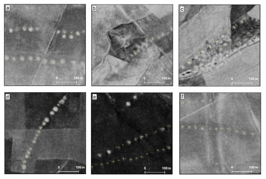
Figure 3.
Qanat shafts, when well preserved (a,d,e) are relatively easy to identify and validate on the CORONA imagery based on the linear alignment of light dots on a darker background. The certainty of identification is lower when preservation is very poor (f) and when natural landscape has a similar signature of white patches on darker background (b,c). In this project, however, shafts with all levels of certainty are labeled and used in training. (Yellow dots are laid over qanat shafts to emphasize the locations of individual shafts.)
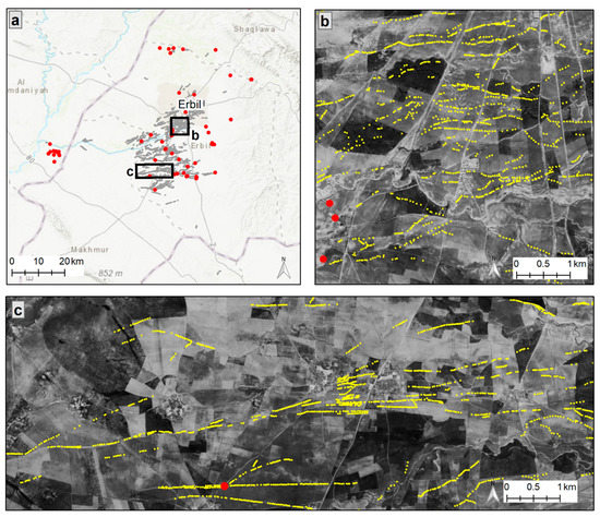
Figure 4.
(a) Overlay of 51 qanats identified by D. Lightfoot from historic documents and field work (red dots) on approximately 12,000 qanat shafts (gray dots) mapped by EPAS at shaft level using historic CORONA imagery. (b,c), enlarged maps for two selected areas illustrate the previous database of qanat (red point) in comparison to the complexity of the qanat landscape captured when shafts are individually identified and mapped (yellow dots). Base Imagery: CORONA frames DS1039-2088DA037 and DS1039-2088DA038, acquired 1968, courtesy of the USGS.
We anticipated that CNNs would have good performance in the detection of qanat shafts. Circular features have proven to yield relatively good results in automated archaeological prospection, in traditional as well as deep learning methods [9,10,12,16,40,45,46,47,61]. Furthermore, unlike most archaeological objects, expensive and time-consuming fieldwork is not crucial for sample data collection and model performance validation. Qanat shafts, especially when well-preserved, are generally easy to identify in any imagery. The shafts are originally doughnut-shaped; the spoil heap from the excavation and maintenance of the shaft creates a ring around the central hole. This circular shape is altered in a variety of ways as soon as the underlying tunnel is out of use, but the shafts maintain a (semi)-circular shape until they disappear. In addition, qanat shafts are found in linear groups, a pattern that is rarely found in nature (Figure 3). Our goal was to test the hypothesis that deep learning can be used for automated detection of archaeological features with relatively uniform signature such as qanat shafts. We aimed at assessing the presence or absence of qanat shafts, not attributes such as shaft size or shape.
Experiments with automated object detection for archaeological prospection have previously been limited to a subset of projects that work with sub-meter and multispectral imagery. This was originally inevitable because traditional algorithms relied heavily on the spectral and high spatial resolution of expensive commercial imagery [11,12,17,22,47,54]. Our second goal was to assess the performance of deep learning in the automated detection on publicly available historic imagery. CORONA satellite imagery is panchromatic with approximately 1.8 m spatial resolution. CORONA is available to all projects and individuals at no or little cost. While the decreasing cost of commercial imagery will make high-resolution imagery more widely available in archaeology, a core area of remote sensing is and will be based on the use of panchromatic low-resolution historic imagery. This is especially the case in developing countries where landscapes are often heavily damaged or destroyed by development projects and thus not captured in the modern imagery [62]. We used CNNs to detect qanat shafts within the area of the Erbil Plain Archaeological Survey.
2. Case Study
The case study is the area covered by the Erbil Plain Archaeological Survey (EPAS) [63]. EPAS encompasses 3200 km2 in the center of the Erbil Governorate of the Kurdistan Region of Iraq (Figure 5). Qanat technology is used in the Kurdistan Region of Iraq, known locally as karez. Karez of Northern Iraq are one of the least-studied qanat systems of the Middle East. The only systematic study of the qanat of Northern Iraq was conducted by Dale Lightfoot under the auspices of UNESCO [64]. He recorded 683 qanat systems, using historic cadastral maps and field observation. One of the largest concentrations of qanat systems is in the EPAS area. Fifty-one qanat systems in the Lightfoot database are within EPAS area. Although the Lightfoot study used cadastral maps, these maps only document the qanat that were functional or recently abandoned in the mid-20th century.
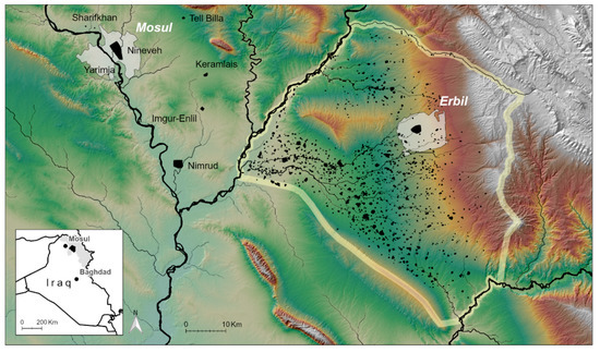
Figure 5.
Erbil Plain Archaeological Survey (EPAS) in the Kurdistan Region of Northern Iraq, marked with black fill on grayscale map and yellow outline on the color map. The archaeological sites recorded by EPAS (2012–2018) are marked with black fill within the EPAS survey area.
Since 2018, EPAS has been investigating the historic qanat systems of the Erbil Plain. The landscape of the plain is heavily altered by anthropological processes, mainly development. Only a small portion, between 5% to 10%, of the shafts visible on the CORONA imagery are preserved and are captured in modern imagery (Figure 6). Declassified Cold War era CORONA imagery were acquired between 1960–1978 and captured the archaeological landscape right before it was heavily altered. In order to document and study the complexity of this qanat landscape, we created a shaft-level map through visual inspection of historic CORONA satellite imagery and manual marking of shafts in a GIS database. Our database contains around 12,000 shafts, some of which belong to the 51 qanat documented earlier and others which were previously undocumented (Figure 4). On the CORONA imagery, the shaft diameter usually ranges between 15 and 25 m, although shafts as small as 10 m and as big as 35 m are found. The process of manual mapping is, however, extremely slow and time consuming. In order to reproduce the depth of this study at a larger scale, we decided to train a deep learning model for automated qanat shaft detection on CORONA imagery that are available for most areas in the Middle East.
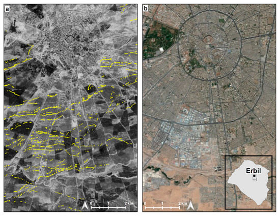
Figure 6.
Using historic satellite imagery is necessary in many areas of the world where processes such as development have destroyed the archaeological record of past landscapes. (a) qanat shafts (yellow dots) abundant south of Erbil on the 1968 CORONA are (b) destroyed by modern development (basemap: ESRI, WorldImagery).
3. Materials and Methods
3.1. Satellite Data
The imagery used for training is the declassified US intelligence imagery from the CORONA program. CORONA acquired photographs from 1960 to 1972 to monitor Soviet missile strength and was declassified in 1995 [65]. Since 1998, archaeologists working in the Middle East have increasingly exploited CORONA imagery because it predates a great deal of landscape destruction by development. In addition, the spatial resolution of the CORONA imagery is high enough to allow for identification of many archaeological features [66]. CORONA imagery can be previewed and ordered on the USGS website (http://earthexplorer.usgs.gov). We downloaded and used the imagery KH-4B (DS1039-2088DA036-039) with a resolution of 1.8 m, acquired in the winter of 1968, when the soil moisture was optimal for remote sensing identification of archaeological landscape features (Table 1).

Table 1.
Location of the 11 patches used for model training on four strips of the CORONA imagery.
3.2. Deep Learning Workflow
A generic machine learning workflow consists of data gathering, data pre-processing, model development, and model evaluation. In data gathering and pre-processing, an annotated data set is created based on ground truth data or expert judgment. Data pre-processing also included exploratory data analysis (EDA) for identification of missing or erroneous annotation cases. To increase training data and to avoid overfitting, data augmentation can be used. Data augmentation generates more training data from existing training samples by random transformations such as image rotation and flipping. Before model development, an evaluation protocol needs to be determined. Once a model is trained, performance metrics are reported based on the evaluation protocol.
3.3. Annotation
Annotation was done by one of the authors who is specialized in remote sensing of landscape irrigation features. For data labeling, we used 3D Slicer, an opensource software platform widely used in medical image processing and annotation [67]. The spatial resolution of the imagery is not enough to create enough padding around each qanat shaft. Therefore, many adjacent qanat shafts were connected in the annotation process, creating clusters of qanat with erroneous variation in size and shape. After the first round of annotation, we conducted exploratory data analysis (EDA) to identify and edit overlapping labels and connected components that would affect the training model performance (Figure 7). Data was labeled for 11 patches that were representative of the diversity of the training contexts. The patches were chosen based on the range of the natural and anthropogenic landscape elements of the Erbil Plain as well as the density and clarity of the qanat shafts (Table 1, Figures S1–S22).
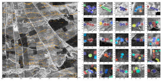
Figure 7.
During data pre-processing, we conducted exploratory data analysis (EDA) to verify that connected components (individual segments) are of reasonable size. Random distinguishing colors were assigned to annotated cases so that outliers and connected components (in the cases where shaft labels overlapped) can be quickly identified. We used this size insight in the post-processing phase to remove some noise. (Note that the left image is flipped vertically in the course of the data augmentation process).
3.4. Convolutional Neural Networks
In this work, a binary classification model based on CNNs is proposed for qanat feature segmentation in CORONA images. Solving an object detection problem with a segmentation framework has been done previously using similar architectures [68,69]. The deep network architecture is composed of sequential convolutional layers . At each convolutional layer , the input feature map (image) is convolved by a set of kernels and biases to generate a new feature map. A non-linear activation function is then applied to this feature map to generate the output which is the input for the next layer. The th feature map of the output of the layer can be expressed by:
The concatenation of the feature maps at each layer provides a combination of patterns to the network, which become increasingly complex for deeper layers. Training of the CNN is usually done with several iterations of stochastic gradient descent (SGD), in which samples of training data (a batch) are processed by the network. At each iteration, based on the calculated loss, the network parameters (kernel weights and biases) are optimized by SGD in order to decrease the loss. Fully convolutional neural networks (FCNs) have been successfully applied in segmentation problems [70,71]. The use of FCNs for image segmentation allows for end-to-end learning, with each pixel of the input image being mapped by the FCN to the output segmentation map. This class of neural networks has shown great success for the task of semantic segmentation. During training, the FCN aims to learn representations based on local information. Although patch-based methods have shown promising results in segmentation tasks, FCNs have the advantage of reducing the computational overhead of sliding-window-based computation. The CNN proposed in this paper is a 2D FCN. FCNs for segmentation consist of an encoder (contracting) path and a decoder (expanding) path. The encoder path consists of repeated convolutional layers followed by activation functions with max-pooling layers on selected feature maps. The encoder path decreases the resolution of the feature maps by computing the maximum of small patches of units of the feature maps. However, good resolution is important for accurate segmentation and therefore up-sampling is performed in the decoder path to restore the initial resolution, but the feature maps are concatenated to keep the computation and memory requirements tractable. As a result of multiple convolutional layers and max-pooling operations, the feature maps are reduced, and the intermediate layers of an FCN become successively smaller. Therefore, following the convolutions, an FCN uses inverse convolutions (or backward convolutions) to up-sample the intermediate layers until the input resolution is matched [72,73]. FCNs with skip-connections are able to combine high-level abstract features with low-level high-resolution features which has been shown to be successful in segmentation tasks [74].
3.5. Network Architecture
Figure 8 illustrates a schematic overview of the anisotropic 3D fully convolutional neural network for qanat feature segmentation in CORONA images. The network architecture is inspired by the 2D U-Net model [52]. The network architecture consists of 22 convolutional, 5 max-pooling, and 5 up-sampling layers. Convolutional layers were applied without padding, while max-pooling layers halved the size of their inputs. The parameters, including the kernel sizes and number of kernels, are explained in each corresponding box. Shortcut connections ensure the combination of low-level and high-level features.
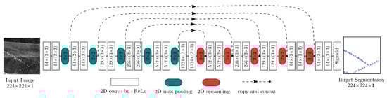
Figure 8.
A schematic overview of the anisotropic 3D fully convolutional neural network for qanat feature segmentation on CORONA images.
As illustrated in Figure 8, each convolution layer has a kernel size of (2 × 2) with a stride of size 1 in the two image dimensions. Since the input of the proposed network is a panchromatic image, the number of channels for the first layer is equal to one. After each convolutional layer, a rectified linear unit (ReLu) is used as the nonlinear activation function except for the last layer where a sigmoid function is used to map the output to a class probability between 0 and 1. There are 5 max-pooling and 5 up-sampling layers of the size 2 × 2 in the encoder and decoder paths, respectively. The network has a total of 31,574,657 trainable parameters. The input to the network is a CORONA image patch , and the output segmentation map size is .
3.6. Training
During training of the proposed network, we aimed to minimize a loss function that measures the quality of the segmentation on the training examples. This loss over N training images can be defined as:
where is the output segmentation map, is the ground truth obtained from expert manual segmentation for the training volume, and (set to 5), is the smoothing coefficient which prevents the denominator from being zero. This loss function has demonstrated utility in image segmentation problems where there is a heavy imbalance between the classes, as in our case where most of the data is considered background [75].
We used a stochastic gradient descent (SGD) algorithm with the Adam update rule [76] which was implemented in the Keras framework (https://github.com/keras-team/keras). The initial learning rate was set to 0.001. The learning rate was reduced by a factor of 0.8 if the average of validation Dice score did not improve by in five epochs. The parameters of the convolutional layers were initialized randomly from a Gaussian distribution using the He method [77]. To prevent overfitting, in addition to batch-normalization [78], we used drop-out with 0.3 probability as well as regularization with penalty on convolutional layers except the last one. Training was performed on eleven 2000 × 2000 CORONA image patches (approximately 5.5 × 5.5 km) using five-fold cross validation (Figure 9).
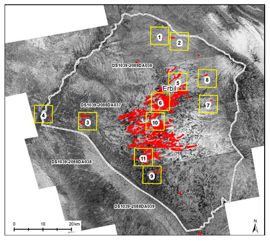
Figure 9.
Approximate location of the 11 training patches.
Each training sample was a 2D patch of the size of pixel. Since grayscale image data encoded as integers in a 0–255 range, we divided each pixel value by 255 to scale the data to the range of [0,1] because neural networks work better with small homogeneous range of values. Data augmentation was performed by equally selecting patches that had qanat and those without qanat and then applying random left-right and up-down flipping of the images. Cross-validation was used to monitor overfitting and to find the best epoch (model checkpoint) for the test-time deployment. For each cross-validation fold, we used 100 as the maximum number of epochs for training and an early stopping policy by monitoring validation performance.
3.7. Postprocessing
At prediction time, a sliding window of 224 × 224 was moved over the 2000 × 2000 image patches with a stride size of 10, and the predictions were summed up. By using a sliding window, predictions with overlapping regions were created that can be viewed as a form of test-time augmentation that can subsequently improve the results. The resultant concatenated prediction map was then thresholded to create the final binary mask prediction denoting the predicted qanat mask. Since we did not have any annotated qanat feature smaller than 10 pixels, we removed any detected features smaller than 10 pixels.
4. Results
We used a five-fold cross-validation to evaluate the model prediction. Table 1 shows patch-by-patch results metrics. Table 2 shows the confusion matrix obtained from the cross-validation process. The overall precision and recall for the model are respectively 0.62 and 0.74. Precision (also known as specificity) measures the proportion of correctly classified positives to all predicted positives. Recall (also known as sensitivity) measures the proportion of correctly classified positives to all annotated positives. Simply put, precision concerns how many predicted cases are correct while recall concerns how many cases of interest are among predictions. The F1 score combines precision and recall in order to balance their importance. The F1 score is the harmonic mean of precision and recall.
Table 2.
Confusion matrix obtained from five-fold cross-validation.
While preparing data for training the model, we decide to include images with both a low and a high density of qanat features. Identifying qanat shafts in low-density photos is a challenging task, even for domain experts. The model performs better on high-density qanat images, defined as containing more than 100 labeled shafts. For five high-density patches (>100 shafts, avg = 704), performance metrics are: precision = 0.654, recall = 0.764, F1 score = 0.705. For six low-density patches (<=100 features, avg = 55), performance metrics are: precision = 0.340, recall = 0.526, F1 score = 0.413. There is not a significant pattern in false positives. They include a range of man-made or natural bumpy features that exist across all parts of the study area. Where the number of qanat shafts is low, these false positives reduce the model’s precision performance. Therefore, there is a strong correlation between model precision and total labeled features in a patch because of the significantly higher proportion of false positives/true positives detected in low-density patches (Figure 10 and Figure 11, Figures S23–S33).
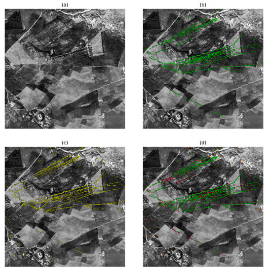
Figure 10.
The highest model performance was on patch 11 (a) with 1178 labeled features, most with high annotation certainty resulting in the highest precision score (0.764) and highest recall score (0.850). (b) Annotated shafts (green), (c) predicted shafts (yellow), (d) evaluation: true positive (TP) (green), false positive (FP) (orange), false negative (FN) (red). Each patch is 2000 × 2000 pixels (approximately 5.5 × 5.5 km).
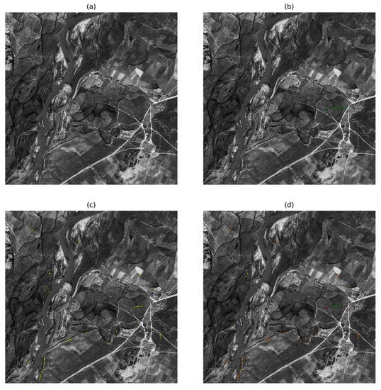
Figure 11.
The lowest model performance was on patch 4 (a) with 23 labeled features, most with low annotation certainty resulting in the lowest precision score (0.107) and very low recall score (0.478). (b) Annotated shafts (green), (c) predicted shafts (yellow), (d) evaluation: TP (green), FP (orange), FN (red). Annotated shafts are only in the center-right part of the image (b), while FP are spread across the lower half of the patch (c). Each patch is 2000 × 2000 pixels (approximately 5.5 × 5.5 km).
5. Discussion
Our project demonstrates that deep learning, even with small datasets, can be successfully applied to automate the detection of qanat shafts. Because qanat infrastructures are found in many countries and contexts and their shafts have similar signatures, it is easy to gradually enlarge the training dataset from a wider range of contexts and optimize the CNNs for this task. In order to illustrate the performance of the CNN model, we chose not to pre-process the imagery and to apply minimal post-processing of the results. These two steps are commonly applied to improve the results in archaeological object detection projects [14,17,51,54]. We also wanted to test automation on a real task at hand. Our domain expert labeled all potential shafts including the faint traces that are not easily recognized unless one is highly experienced with the signature and patterns of the qanat on the imagery. We expected that the model would have performed even better if the training dataset were limited to the relatively well-preserved shafts (see above).
We had envisioned that selecting training data from a wide range of locations in the study area would improve the model’s performance (Figure 9). However, the fact that seven out of eleven patches were in the low-density shaft zones seem to have negatively affected our model performance. Probably, with larger datasets, diversifying the annotation context would improve the model. However, in our case, we concluded that limiting the labeled data on the high-density qanat areas would have focused the model on learning local features of those areas and would have yielded better results. Although the number of false positives is reasonably low, the worst performance is observed in low-density patches. Our model demonstrated better recall performance than precision. In ten out of eleven patches, at least half of the labeled objects were detected.
Qanats can be largely validated with visual inspection because shafts are found in long and linear alignments. In most landscapes, including on the Erbil Plain, only a small proportion of the shafts are preserved, and thus it is not possible to ground-truth the qanat beyond visual inspection. The creation of large, high-quality training datasets will be one of the biggest challenges along the way for archaeological prospection tasks using deep learning. In order to increase the recall rate, objects with lower certainty levels need to be labeled. The uncertainties, bias, and error during the labeling process will affect the model performance. Without ground-truthed labeled data, it is hard to judge where errors in training data may have contributed to the weak performance of the model. For example, our model performed best in areas were shafts are abundant and better preserved. The highest rate of false positives to true positives were in areas where qanat shafts are rare or the certainty of identification is low.
The existing model can be improved if a larger training dataset of field-validated data is available. From an engineering point of view, we envision experimentation toward improving the model itself through the following methods. First, we can experiment with a classification method, rather than the segmentation that is used in the existing model. Two deep learning methods of segmentation and classification could be applied to automatic detection of objects in remote sensing data. Segmentation implements a binary classification at pixel level. The outcome is either yes, i.e., the pixel belongs to an object of interest, or no, i.e., the pixel does not. Classification identifies an object, composed of any number of pixels, and determines whether the object belongs to any of the defined object classes (see for example [61]). Since the visibility of the entire object is not crucial in segmentation, we anticipate that it could perform better with lower resolution imagery. However, further work needs to be carried out to assess the capability of deep learning methods for the accurate segmentation of shaft boundaries which can provide useful archaeological information about the size and shape of shafts. Architectures such as the U-Net that was used in this paper or Mask R-CNNs [79] can be used for such segmentation tasks. Using Mask R-CNNs has the advantage of predicting bounding boxes and segmentation masks simultaneously. We also envision experimentation with classification to compare the results of the two approaches. Second, we will also investigate ways to improve the performance of the proposed CNN architecture. In this work, we used a baseline model very similar to the U-Net architecture and we trained the whole network from scratch. Transfer learning by using pre-trained ImageNet models for the encoder section of U-Net has been successful in some segmentation applications [80]. We will run experiments to compare U-Nets with pre-trained encoders with the baseline architecture reported here. Third, we will study the ability of the proposed model in predictive uncertainty estimation and will try confidence calibration to improve it [81].
In the short term, however, we have three immediate concerns. First, we plan to integrate post-processing measures that may be able to improve the rate of true to false positives. Although detection performance is routinely reported through metrics such as recall and precision, the most important metric is how well the model is suited for a specific task. High metrics can be achieved for models that are trained for a small task with no outside application [12,50]. When models are trained for a complex task across a big region, better performance is achieved if the certainty measures are relaxed to increase recall, and quick post-processing steps are integrated to increase precision [51]. In our case, for example, we may be able to eliminate false positives based on the nearby positives. Second, we aim to build other pieces of the workflow that are necessary in order to transform the pixel-value results of the segmentation process into localized vector files that can be imported into a GIS environment. Third, we plan to test our existing model in automated detection of qanats in other regions without labeling new data in order to compare the performance of our model in familiar and new landscapes.
6. Conclusions
Deep learning has proved to be a powerful method for challenging computer vision tasks. In fields as sensitive as cancer diagnosis, deep learning has proved to create results superior to novice expert and comparable to experienced experts [53]. It is outdated to debate whether archaeology should embrace automated detection. Instead, the focus must be on how to embrace the soon-to-be ubiquitous deep learning tools in order to overcome the challenges of data overload and to speed up the process of remote-sensing documentation in the face of increasingly rapid destruction of the archaeological landscapes. Automated detection is not a replacement for human experts. By eliminating manual tasks that can be delegated to computers, the researcher’s precious and limited time can be focused on the validation and analysis of the results. Furthermore, automation will open new research opportunities, for example for in-depth large-scale landscape study of regional-scale features with relatively uniform appearance [9,11], such as qanats. Automation will open new research opportunities that are currently unfeasible. For example, a regional-scale comparative study of qanat technology is currently impossible because no one has the time to create detailed maps of qanat shafts manually. It is possible to use transfer learning and data augmentation to overcome the problem of small datasets for archaeological prospection tasks.
So far, all archaeological experimentation has used models trained for other tasks. However, once more projects integrate deep learning and larger datasets are available, CNN models could be optimized for archaeological remote-sensing autodetection tasks, and we would witness even better results. The promising performance of deep learning has encouraged some researchers to build in-house tools for specific archaeological tasks [22]. Another possible direction is that commercial off-the-shelf deep-learning platforms that are emerging for industrial applications can be soon used for archaeological tasks as well.
Supplementary Materials
The following are available online at https://www.mdpi.com/2072-4292/12/3/500/s1, Figures S1–S22, location of training patches on the CORONA image sections. Figures S23–S33, Training results on individual patches: (a) original patch, (b) annotated shafts (green), (c) predicted shafts (yellow), (d) evaluation: TP (green), FP (orange), FN (red).
Author Contributions
Conceptualization, all authors; methodology, all authors; software, A.M. and E.K.; validation, M.S., A.M., E.K.; formal analysis, A.M., and E.K., M.S.; data curation, M.S., A.M.; writing—original draft preparation, M.S., E.K., and A.M.; writing—review and editing, all authors; visualization, M.S., A.M., E.K.; project administration, M.S. All authors have read and agreed to the published version of the manuscript.
Funding
This research was in part funded by the US National Science Foundation (Award 1261118), National Geographic Society, the US National Institutes of Health (Grant P41EB015898), Natural Sciences and Engineering Research Council (NSERC) of Canada, and the Canadian Institutes of Health Research (CIHR).
Acknowledgments
The authors would like to thank Dale Lightfoot for providing the schematic diagram of a qanat. EPAS would like to express its gratitude for the help and encouragement of the following institutions and individuals from the Kurdistan Regional Government, Iraq: General Directorate of Antiquities, in particular its current director Kak Kaifi Ali and its former director Kak Abubakir Othman Zainaddin (Mala Awat), Directorate of Antiquities, Erbil Governorate, its director Kak Nader Babakr, and our representative Kak Khalil Barzinji.
Conflicts of Interest
The authors declare no conflict of interest.
References
- Wiseman, J.R.; El-Baz, F. Remote Sensing in Archaeology; Springer Science & Business Media: Berlin/Heidelberg, Germany, 2007. [Google Scholar]
- Parcak, S.H. Satellite Remote Sensing for Archaeology; Routledge: London, UK; New York, NY, USA, 2009. [Google Scholar]
- Lasaponara, R.; Masini, N. Satellite Remote Sensing:A New Tool for Archaeology; Remote Sensing and Digital Image Processing; Springer: Dordrecht, The Netherlands, 2012; Volume 16. [Google Scholar]
- Leisz, S.J. An Overview of the Application of Remote Sensing to Archaeology During the Twentieth Century. In Mapping Archaeological Landscapes from Space; Douglas, C., Comer, D.C., Harrower, M.J., Eds.; Springer: New York, NY, USA, 2013. [Google Scholar]
- Hritz, C. Tracing Settlement Patterns and Channel Systems in Southern Mesopotamia Using Remote Sensing. J. Field Archaeol. 2010, 35, 184–203. [Google Scholar] [CrossRef]
- Bewley, B.; Bradbury, J. The Endangered Archaeology in the Middle East and North Africa Project: Origins, Development and Future Directions. Bull. Counc. Br. Res. Levant 2017, 12, 15–20. [Google Scholar] [CrossRef]
- Hammer, E.; Seifried, R.; Franklin, K.; Lauricella, A. Remote Assessments of the Archaeological Heritage Situation in Afghanistan. J. Cult. Herit. 2018, 33, 125–144. [Google Scholar] [CrossRef]
- Franklin, K.; Hammer, E. Untangling Palimpsest Landscapes in Conflict Zones: A “Remote Survey” in Spin Boldak, Southeast Afghanistan. J. Field Archaeol. 2018, 43, 58–73. [Google Scholar] [CrossRef]
- Cowley, D.C. In with the New, out with the Old? Auto-Extraction for Remote Sensing Archaeology. In Remote Sensing of the Ocean, Sea Ice, Coastal Waters, and Large Water Regions; Bostater, C.R., Mertikas, S.P., Neyt, X., Nichol, C., Cowley, D., Bruyant, J.-P., Eds.; Proceedings of SPIE; International Society for Optics and Photonics: Edinburgh, UK, 2012; Volume 8532, p. 853206. [Google Scholar] [CrossRef]
- Trier, Ø.D.; Pilø, L.H.; Johansen, H.M. Semi-Automatic Mapping of Cultural Heritage from Airbone Laser Scanning Data. Semata Cienc. Sociais Humanid. 2015, 27, 159–186. [Google Scholar]
- Lambers, K.; Verschoof-van der Vaart, W.; Bourgeois, Q. Integrating Remote Sensing, Machine Learning, and Citizen Science in Dutch Archaeological Prospection. Remote Sens. 2019, 11, 794. [Google Scholar] [CrossRef]
- Trier, Ø.D.; Cowley, D.C.; Waldeland, A.U. Using Deep Neural Networks on Airborne Laser Scanning Data: Results from a Case Study of Semi-automatic Mapping of Archaeological Topography on Arran, Scotland. Archaeol. Prospect. 2019, 26, 165–175. [Google Scholar] [CrossRef]
- Traviglia, A.; Cowley, D.; Lambers, K. Finding Common Ground: Human and Computer Vision in Archaeological Prospection. AARGnews 2016, 53, 11–24. [Google Scholar]
- Bennett, R.; Cowley, D.; De Laet, V. The Data Explosion: Tackling the Taboo of Automatic Feature Recognition in Airborne Survey Data. Antiquity 2014, 88, 896–905. [Google Scholar] [CrossRef]
- Schuetter, J.; Goel, P.; Mccorriston, J.; Park, J.; Senn, M.; Harrower, M. Autodetection of Ancient Arabian Tombs in High-Resolution Satellite Imagery. Int. J. Remote Sens. 2013, 34, 6611–6635. [Google Scholar] [CrossRef]
- Trier, Ø.D.; Larsen, S.Ø.; Solberg, R. Automatic Detection of Circular Structures in High-Resolution Satellite Images of Agricultural Land. Archaeol. Prospect. 2009, 16, 1–15. [Google Scholar] [CrossRef]
- Zingman, I.; Saupe, D.; Penatti, O.A.B.; Lambers, K. Detection of Fragmented Rectangular Enclosures in Very High Resolution Remote Sensing Images. IEEE Trans. Geosci. Remote Sens. 2016, 54, 4580–4593. [Google Scholar] [CrossRef]
- Lambers, K.; Zingman, I. Towards Detection of Archaeological Objects in High-Resolution Remotely Sensed Images: The Silvretta Case Study. In Proceedings of the Archaeology in the Digital Era: Papers from the 40th Annual Conference of Computer Applications and Quantitative Methods in Archaeology (CAA), Southampton, UK, 26–29 March 2012; Verhagen, P., Earl, G., Chrysanthi, A., Murrieta-Flores, P., Papadopoulos, C., Romanowska, I., Wheatley, D., Eds.; University Press: Amsterdam, The Netherlands, 2014; pp. 781–791. [Google Scholar]
- De Laet, V.; Paulissen, E.; Waelkens, M. Methods for the Extraction of Archaeological Features from Very High-Resolution Ikonos-2 Remote Sensing Imagery, Hisar (Southwest Turkey). J. Archaeol. Sci. 2007, 34, 830–841. [Google Scholar] [CrossRef]
- Casana, J. Regional-Scale Archaeological Remote Sensing in the Age of Big Data. Adv. Archaeol. Pract. 2014, 2, 222–233. [Google Scholar] [CrossRef]
- Cowley, D.C.; Palmer, R. Interpreting Aerial Images—Developing Best Practice. In Space, Time and Place, Proceedings of the III International Conference on Remote Sensing in Archaeology, Tirucirapalli, India, 17–21 August 2009; Forte, M., Campana, S., Liuzza, C., Eds.; BAR International Series; Archaeopress: Oxford, UK, 2010; pp. 129–135. [Google Scholar]
- Verschoof-van der Vaart, W.B.; Lambers, K. Learning to Look at LiDAR: The Use of R-CNN in the Automated Detection of Archaeological Objects in LiDAR Data from the Netherlands. J. Comput. Appl. Archaeol. 2019, 2, 31–40. [Google Scholar] [CrossRef]
- Bajcsy, R.; Tavakoli, M. Computer Recognition of Roads from Satellite Pictures. IEEE Trans. Syst. Man Cybern. 1976, 6, 623–637. [Google Scholar] [CrossRef]
- Bajcsy, R.; Tavakoli, M. A Computer Recognition of Bridges, Islands, Rivers and Lakes from Satellite Pictures. In Proceedings of the Conference on Machine Processing of Remotely Sensed Data, West Lafayette, IN, USA, 16–18 October 1973. [Google Scholar]
- Vanderbrug, G.; Rosenfeld, A. Linear Feature Mapping. IEEE Trans. Syst. Man Cybern. 1978, 8, 768–774. [Google Scholar]
- Fischler, M.A.; Tenenbaum, J.M.; Wolf, H.C. Detection of Roads and Linear Structures in Low-Resolution Aerial Imagery Using a Multisource Knowledge Integration Technique. Comput. Graph. Image Process. 1981, 15, 201–223. [Google Scholar] [CrossRef]
- Bhattacharya, U.; Parui, S.K. An Improved Backpropagation Neural Network for Detection of Road-like Features in Satellite Imagery. Int. J. Remote Sens. 1997, 18, 3379–3394. [Google Scholar] [CrossRef]
- Mayer, H. Automatic Object Extraction from Aerial Imagery—A Survey Focusing on Buildings. Comput. Vis. Image Underst. 1999, 74, 138–149. [Google Scholar] [CrossRef]
- Kim, T.; Muller, J.-P. Development of a Graph-Based Approach for Building Detection. Image Vis. Comput. 1999, 17, 3–14. [Google Scholar] [CrossRef]
- Krishnamachari, S.; Chellappa, R. Delineating Buildings by Grouping Lines with MRFs. IEEE Trans. Image Process. 1996, 5, 164–168. [Google Scholar] [CrossRef] [PubMed]
- Jung, C.R.; Schramm, R. Rectangle Detection Based on a Windowed Hough Transform. In Proceedings of the 17th Brazilian Symposium on Computer Graphics and Image Processing, Curitiba, Brazil, 17–20 October 2004; pp. 113–120. [Google Scholar] [CrossRef]
- Sirmacek, B.; Unsalan, C. Urban-Area and Building Detection Using SIFT Keypoints and Graph Theory. IEEE Trans. Geosci. Remote Sens. 2009, 47, 1156–1167. [Google Scholar] [CrossRef]
- Sirmacek, B.; Unsalan, C. A Probabilistic Framework to Detect Buildings in Aerial and Satellite Images. IEEE Trans. Geosci. Remote Sens. 2011, 49, 211–221. [Google Scholar] [CrossRef]
- Moon, H.; Chellappa, R.; Rosenfeld, A. Optimal Edge-Based Shape Detection. IEEE Trans. Image Process. 2002, 11, 1209–1227. [Google Scholar] [CrossRef]
- Lambers, K.; Traviglia, A. Automated Detection in Remote Sensing Archaeology: A Reading List. AARGnews Newsl. Aer. Archaeol. Res. Group 2016, 53, 25–29. [Google Scholar]
- Lambers, K. Airborne and Spaceborne Remote Sensing and Digital Image Analysis in Archaeology. In Digital Geoarchaeology: New Techniques for Interdisciplinary Human-Environmental Research; Siart, C., Forbriger, M., Bubenzer, O., Eds.; Springer: New York, NY, USA, 2018; pp. 109–122. [Google Scholar]
- De Laet, V.; Lambers, K. Archaeological Prospecting Using High-Resolution Digital Satellite Imagery: Recent Advances and Future Prospects; a Session Held at the Computer Applications and Quantitative Methods in Archaeology (CAA) Conference, Williamsburg, USA, March 2009. AARGnews Newsl. Aer. Archaeol. Res. Group 2009, 9–17. [Google Scholar]
- Trier, Ø.D.; Salberg, A.-B.; Pilø, L.H. Semi-Automatic Detection of Charcoal Kilns from Airborne Laser Scanning Data. In CAA2016: Oceans of Data, Proceedings of the 44th Conference on Computer Applications and Quantitative Methods in Archaeology, Oslo, Norway, 30 March–3 April 2016; Archaeopress Archaeology: Oxford, UK, 2016; pp. 219–231. [Google Scholar]
- Cerrillo-Cuenca, E. An Approach to the Automatic Surveying of Prehistoric Barrows through LiDAR. Quat. Int. 2017, 435, 135–145. [Google Scholar] [CrossRef]
- Schneider, A.; Takla, M.; Nicolay, A.; Raab, A.; Raab, T. A Template-Matching Approach Combining Morphometric Variables for Automated Mapping of Charcoal Kiln Sites: Automated Mapping of Charcoal Kiln Sites. Archaeol. Prospect. 2015, 22, 45–62. [Google Scholar] [CrossRef]
- Freeland, T.; Heung, B.; Burley, D.V.; Clark, G.; Knudby, A. Automated Feature Extraction for Prospection and Analysis of Monumental Earthworks from Aerial LiDAR in the Kingdom of Tonga. J. Archaeol. Sci. 2016, 69, 64–74. [Google Scholar] [CrossRef]
- Menze, B.; Ur, J.; Sherratt, A. Detection of Ancient Settlement Mounds: Archaeological Survey Based on the SRTM Terrain Model. Photogramm. Eng. Remote Sens. 2006, 72, 321–327. [Google Scholar] [CrossRef]
- Luo, L.; Wang, X.; Guo, H.; Liu, C.; Liu, J.; Li, L.; Du, X.; Qian, G. Automated Extraction of the Archaeological Tops of Qanat Shafts from VHR Imagery in Google Earth. Remote Sens. 2014, 6, 11956–11976. [Google Scholar] [CrossRef]
- Trier, Ø.D.; Pilø, L.H. Automatic Detection of Pit Structures in Airborne Laser Scanning Data. Archaeol. Prospect. 2012, 19, 103–121. [Google Scholar] [CrossRef]
- Toumazet, J.-P.; Vautier, F.; Roussel, E.; Dousteyssier, B. Automatic Detection of Complex Archaeological Grazing Structures Using Airborne Laser Scanning Data. J. Archaeol. Sci. Rep. 2017, 12, 569–579. [Google Scholar] [CrossRef]
- Sevara, C.; Pregesbauer, M.; Doneus, M.; Verhoeven, G.; Trinks, I. Pixel versus Object—A Comparison of Strategies for the Semi-Automated Mapping of Archaeological Features Using Airborne Laser Scanning Data. J. Archaeol. Sci. Rep. 2016, 5, 485–498. [Google Scholar] [CrossRef]
- Trier, Ø.D.; Salberg, A.-B.; Pilø, L.H. Semi-Automatic Mapping of Charcoal Kilns from Airborne Laser Scanning Data Using Deep Learning. In Oceans of Data, Proceedings of the 44th Conference on Computer Applications and Quantitative Methods in Archaeology, Tübingen, Germany, 19–23 March 2018; Matsumoto, M., Uleberg, E., Eds.; Archaeopress Archaeology: Oxford, UK, 2018; pp. 219–231. [Google Scholar]
- Menze, B.H.; Ur, J.A. Mapping Patterns of Long-Term Settlement in Northern Mesopotamia at a Large Scale. Proc. Natl. Acad. Sci. USA 2012, 109, E778–E787. [Google Scholar] [CrossRef]
- Caspari, G.; Balz, T.; Gang, L.; Wang, X.; Liao, M. Application of Hough Forests for the Detection of Grave Mounds in High-Resolution Satellite Imagery. In Proceedings of the IEEE Geoscience and Remote Sensing Symposium, Quebec City, QC, Canada, 13–18 July 2014; pp. 906–909. [Google Scholar] [CrossRef]
- Guyot, A.; Hubert-Moy, L.; Lorho, T. Detecting Neolithic Burial Mounds from LiDAR-Derived Elevation Data Using a Multi-Scale Approach and Machine Learning Techniques. Remote Sens. 2018, 10, 225. [Google Scholar] [CrossRef]
- Mnih, V.; Hinton, G.E. Learning to Detect Roads in High-Resolution Aerial Images. In Computer Vision—ECCV 2010, Proceedings of the 11th European Conference on Computer Vision, Heraklion, Greece, 5–11 September 2010; Daniilidis, K., Maragos, P., Paragios, N., Eds.; Springer: Berlin/Heidelberg, Germany, 2010; Volume 6316, pp. 210–223. [Google Scholar] [CrossRef]
- Krizhevsky, A.; Sutskever, I.; Hinton, G.E. ImageNet Classification with Deep Convolutional Neural Networks. In Advances in Neural Information Processing Systems 25, Proceedings of the 26th Annual Conference on Neural Information Processing Systems 2012, Lake Tahoe, NV, USA, 3–6 December 2012; Pereira, F., Burges, C.J.C., Bottou, L., Weinberger, K.Q., Eds.; Curran Associates Inc.: Red Hook, NY, USA, 2012; pp. 1097–1105. [Google Scholar]
- Bi, W.L.; Hosny, A.; Schabath, M.B.; Giger, M.L.; Birkbak, N.J.; Mehrtash, A.; Allison, T.; Arnaout, O.; Abbosh, C.; Dunn, I.F.; et al. Artificial Intelligence in Cancer Imaging: Clinical Challenges and Applications. CA Cancer J. Clin. 2019, 69, 127–157. [Google Scholar] [CrossRef]
- Salberg, A.-B.; Trier, Ø.D.; Kampffmeyer, M. Large-Scale Mapping of Small Roads in Lidar Images Using Deep Convolutional Neural Networks. In Image Analysis, Proceedings of the 20th Scandinavian Conference, SCIA 2017, Tromsø, Norway, 12–14 June 2017; Sharma, P., Bianchi, F.M., Eds.; Springer International Publishing: Cham, Switzerland, 2017; Volume 10270, pp. 193–204. [Google Scholar] [CrossRef]
- Beaumont, P.; Bonine, M.E.; McLachlan, K.S.; McLachlan, A. Qanat, Kariz, and Khattara: Traditional Water Systems in the Middle East. and North. Africa; Middle East Centre, School of Oriental and African Studies, University of London: London, UK; Middle East & North African Studies Press: Wisbech, UK, 1989. [Google Scholar]
- English, P.W. The Origin and Spread of Qanats in the Old World. Proc. Am. Philos. Soc. 1968, 112, 170–181. [Google Scholar]
- Goblot, H. Les Qanats: Une Technique D’acquisition de L’eau; Industrie et artisanat; Mouton: Paris, France; New York, NY, USA, 1979. [Google Scholar]
- Boucharlat, R. Qanat and Falaj: Polycentric and Multi-Period Innovations Iran and the United Arab Emirates as Case Studies. In Underground Aqueducts Handbook; CRC Press: Boca Raton, FL, USA, 2016; pp. 279–304. [Google Scholar] [CrossRef]
- Magee, P. The Chronology and Environmental Background of Iron Age Settlement in Southeastern Iran and the Question of the Origin of the Qanat Irrigation System. Iran. Antiq. 2005, 40, 217–231. [Google Scholar] [CrossRef]
- Charloux, G.; Courbon, P.; Testa, O.; Thomas, M. Mapping an Ancient Qanat System in a Northern Arabian Urbanized Oasis. Water Hist. 2018, 10, 31–51. [Google Scholar] [CrossRef]
- Kermit, M.; Hamar, J.B.; Trier, Ø.D. Towards a National Infrastructure for Semi-Automatic Mapping of Cultural Heritage in Norway. In Oceans of Data, Proceedings of the 44th Conference on Computer Applications and Quantitative Methods in Archaeology, Tübingen, Germany, 19–23 March 2018; Matsumoto, M., Uleberg, E., Eds.; Archaeopress: Oxford, UK, 2018; pp. 159–172. [Google Scholar]
- Comer, D.C.; Harrower, M.J. Mapping Archaeological Landscapes from Space; Springer: New York, NY, USA, 2013. [Google Scholar]
- Ur, J.A.; De Jong, L.; Giraud, J.; Osborne, J.F.; MacGinnis, J. Ancient Cities and Landscapes in the Kurdistan Region of Iraq: The Erbil Plain Archaeological Survey 2012 Season. Iraq 2013, 75, 89–117. [Google Scholar] [CrossRef]
- Lightfoot, D. Survey of Infiltration Karez in Northern Iraq: History and Current Status of Underground Aqueducts; A Report Prepared for UNESCO; UNESCO: Paris, France, 2009. [Google Scholar]
- Ruffner, K.C. Corona America’s First Satellite Program; History Staff, Center for the Study of Intelligence, Central Intelligence Agency: Washington, DC, USA, 1995. [Google Scholar]
- Ur, J.A. CORONA Satellite Imagery and Ancient Near Eastern Landscapes. In Mapping Archaeological Landscapes from Space; Comer, D.C., Harrower, M.J., Eds.; Springer: New York, NY, USA, 2013; pp. 21–32. [Google Scholar]
- Kikinis, R.; Pieper, S.D.; Vosburgh, K.G. 3D Slicer: A Platform for Subject-Specific Image Analysis, Visualization, and Clinical Support. In Intraoperative Imaging and Image-Guided Therapy; Jolesz, F.A., Ed.; Springer: New York, NY, USA, 2014; pp. 277–289. [Google Scholar] [CrossRef]
- Liao, H.; Mesfin, A.; Luo, J. Joint Vertebrae Identification and Localization in Spinal CT Images by Combining Short- and Long-Range Contextual Information. IEEE Trans. Med. Imaging 2018, 37, 1266–1275. [Google Scholar] [CrossRef] [PubMed]
- Zaffino, P.; Pernelle, G.; Mastmeyer, A.; Mehrtash, A.; Zhang, H.; Kikinis, R.; Kapur, T.; Francesca Spadea, M. Fully Automatic Catheter Segmentation in MRI with 3D Convolutional Neural Networks: Application to MRI-Guided Gynecologic Brachytherapy. Phys. Med. Biol. 2019, 64, 165008. [Google Scholar] [CrossRef] [PubMed]
- Ronneberger, O.; Fischer, P.; Brox, T. U-Net: Convolutional Networks for Biomedical Image Segmentation. In Medical Image Computing and Computer-Assisted Intervention—MICCAI 2015, Proceedings of the 18th International Conference, Munich, Germany, 5–9 October 2015; Navab, N., Hornegger, J., Wells, W.M., Frangi, A.F., Eds.; Lecture Notes in Computer Science; Springer International Publishing: Berlin/Heidelberg, Germany, 2015; pp. 234–241. [Google Scholar]
- Badrinarayanan, V.; Kendall, A.; Cipolla, R. SegNet: A Deep Convolutional Encoder-Decoder Architecture for Image Segmentation. IEEE Trans. Pattern Anal. Mach. Intell. 2017, 39, 2481–2495. [Google Scholar] [CrossRef] [PubMed]
- Shelhamer, E.; Long, J.; Darrell, T. Fully Convolutional Networks for Semantic Segmentation. IEEE Trans. Pattern Anal. Mach. Intell. 2017, 39, 640–651. [Google Scholar] [CrossRef] [PubMed]
- Eigen, D.; Puhrsch, C.; Fergus, R. Depth Map Prediction from a Single Image Using a Multi-Scale Deep Network. In Proceedings of the 27th International Conference on Neural Information Processing Systems, NIPS’14, Montreal, QC, Canada, 8–13 December 2014; MIT Press: Cambridge, MA, USA, 2014; Volume 2, pp. 2366–2374. [Google Scholar]
- Çiçek, Ö.; Abdulkadir, A.; Lienkamp, S.S.; Brox, T.; Ronneberger, O. 3D U-Net: Learning Dense Volumetric Segmentation from Sparse Annotation. In Proceedings of the International Conference on Medical Image Computing and Computer-Assisted Intervention, Athens, Greece, 17–21 October 2016. [Google Scholar]
- Milletari, F.; Navab, N.; Ahmadi, S. V-Net: Fully Convolutional Neural Networks for Volumetric Medical Image Segmentation. In Proceedings of the Fourth International Conference on 3D Vision (3DV), Stanford, CA, USA, 25–28 October 2016; pp. 565–571. [Google Scholar] [CrossRef]
- Kingma, D.P.; Ba, J. Adam: A Method for Stochastic Optimization. arXiv 2014, arXiv:1412.6980. [Google Scholar]
- He, K.; Zhang, X.; Ren, S.; Sun, J. Delving Deep into Rectifiers: Surpassing Human-Level Performance on ImageNet Classification. In Proceedings of the IEEE International Conference on Computer Vision (ICCV), Santiago, Chile, 7–13 December 2015; pp. 1026–1034. [Google Scholar] [CrossRef]
- Ioffe, S.; Szegedy, C. Batch Normalization: Accelerating Deep Network Training by Reducing Internal Covariate Shift. arXiv 2015, arXiv:1502.03167. [Google Scholar]
- He, K.; Gkioxari, G.; Dollár, P.; Girshick, R. Mask R-CNN. arXiv 2018, arXiv:1703.06870. [Google Scholar]
- Iglovikov, V.; Shvets, A. TernausNet: U-Net with VGG11 Encoder Pre-Trained on ImageNet for Image Segmentation. arXiv 2018, arXiv:1801.05746. [Google Scholar]
- Guo, C.; Pleiss, G.; Sun, Y.; Weinberger, K.Q. On Calibration of Modern Neural Networks. arXiv 2017, arXiv:1706.04599. [Google Scholar]
© 2020 by the authors. Licensee MDPI, Basel, Switzerland. This article is an open access article distributed under the terms and conditions of the Creative Commons Attribution (CC BY) license (http://creativecommons.org/licenses/by/4.0/).