LiCSBAS: An Open-Source InSAR Time Series Analysis Package Integrated with the LiCSAR Automated Sentinel-1 InSAR Processor

 , , and
Abstract
:
1. Introduction
2. LiCSAR and LiCSBAS
2.1. LiCSAR: Automatic Sentinel-1 InSAR Processer
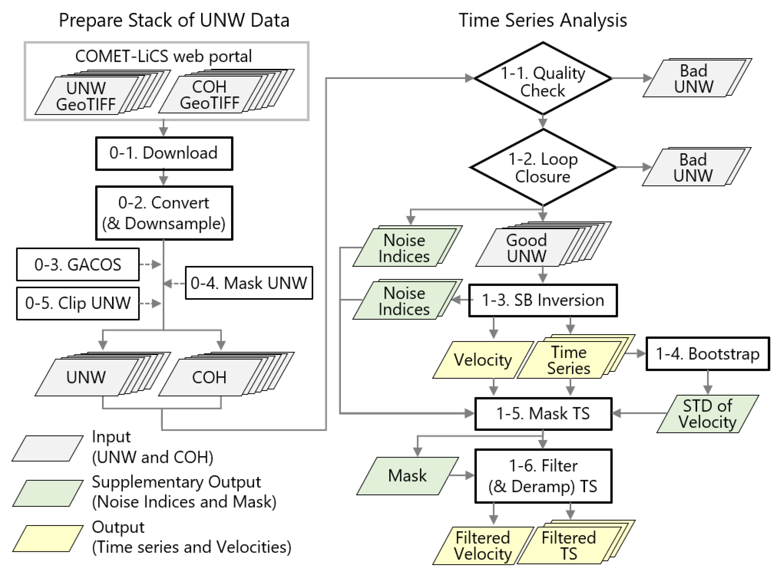
2.2. LiCSBAS Overview
2.3. Prepare Stack of Unwrapped Data
2.3.1. Step 0-1: Download LiCSAR Products
2.3.2. Step 0-2: Convert GeoTIFF (and Downsample)
2.3.3. Step 0-3: Tropospheric Noise Correction Using GACOS (Optional)
2.3.4. Step 0-4: Mask Interferograms (Optional)
2.3.5. Step 0-5: Clip Interferograms (Optional)
2.4. Time Series Analysis
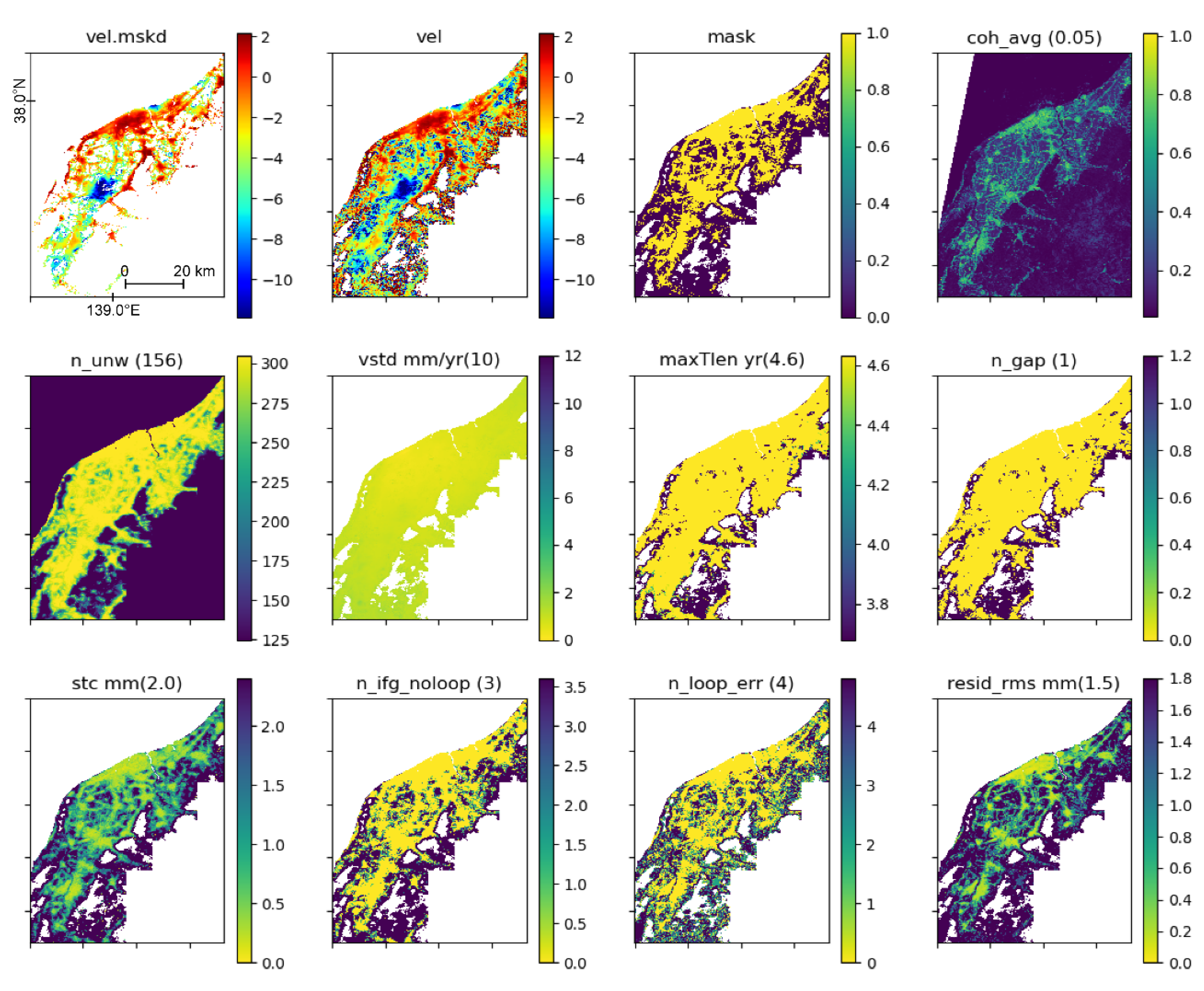
2.4.1. Step 1-1: Quality Check
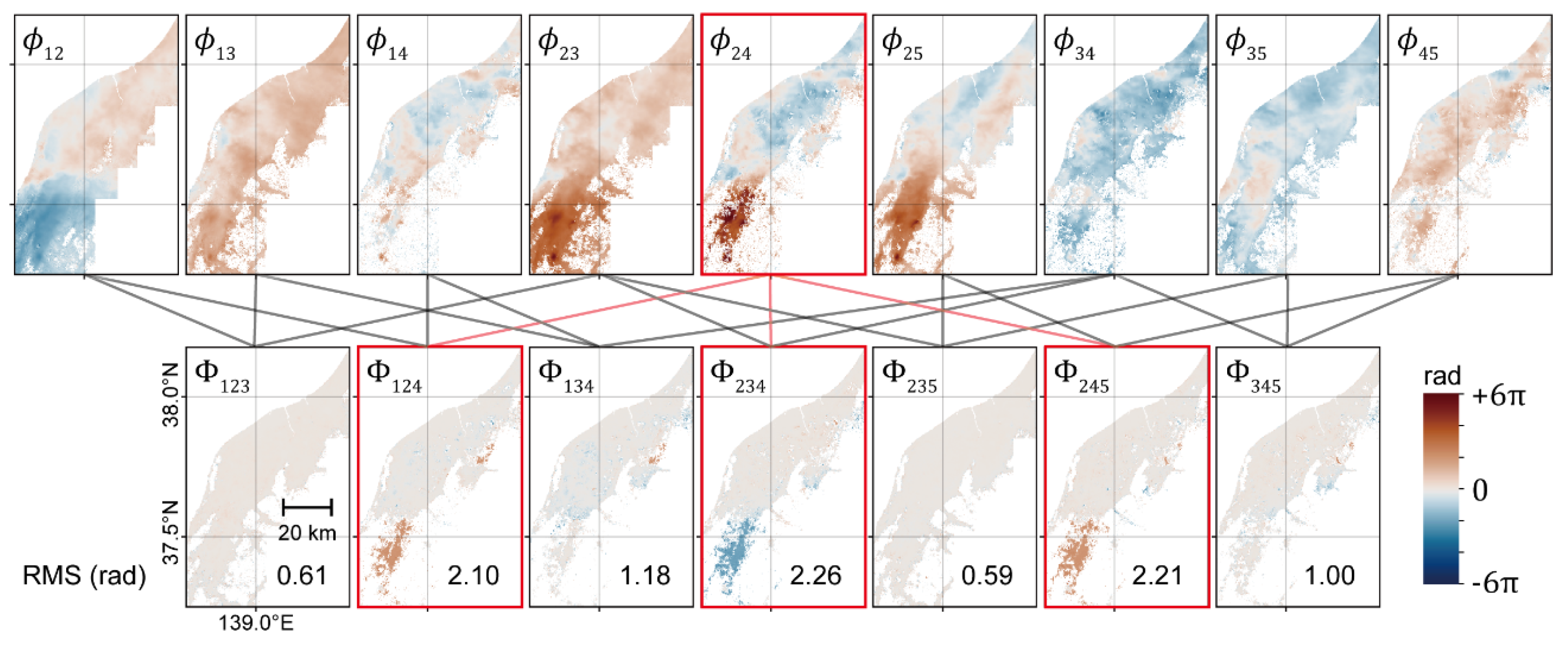
2.4.2. Step 1-2: Network Refinement by Loop Closure
2.4.3. Step 1-3: Small Baseline Network Inversion
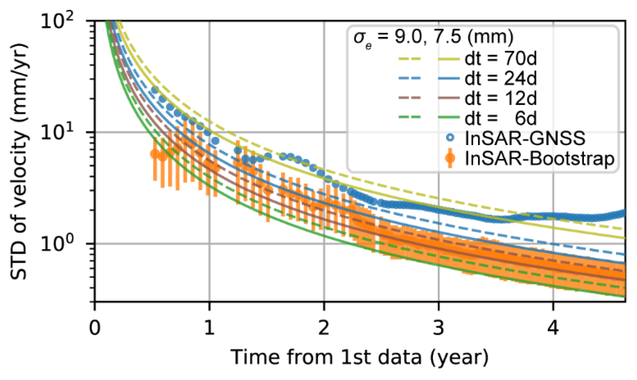
2.4.4. Step 1-4: Estimate Standard Deviation of the Velocity by Bootstrap
2.4.5. Step 1-5: Mask Noisy Pixels in the Time Series
2.4.6. Step 1-6: Spatiotemporal Filtering of Time Series
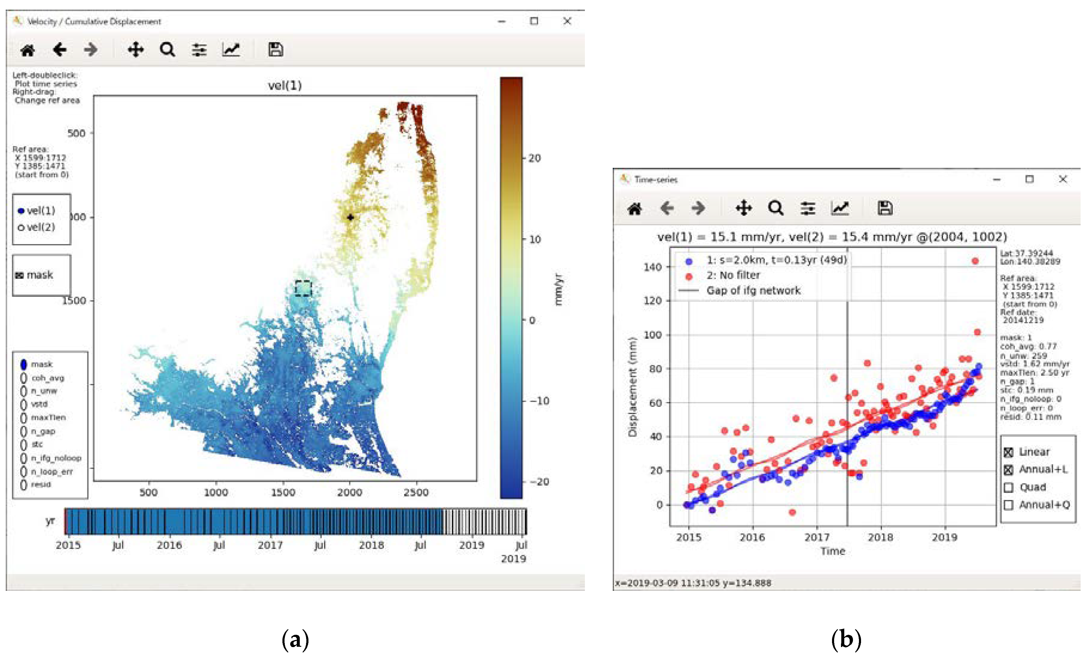
2.5. Visualization of the Results
3. Case Study: Entire Frame
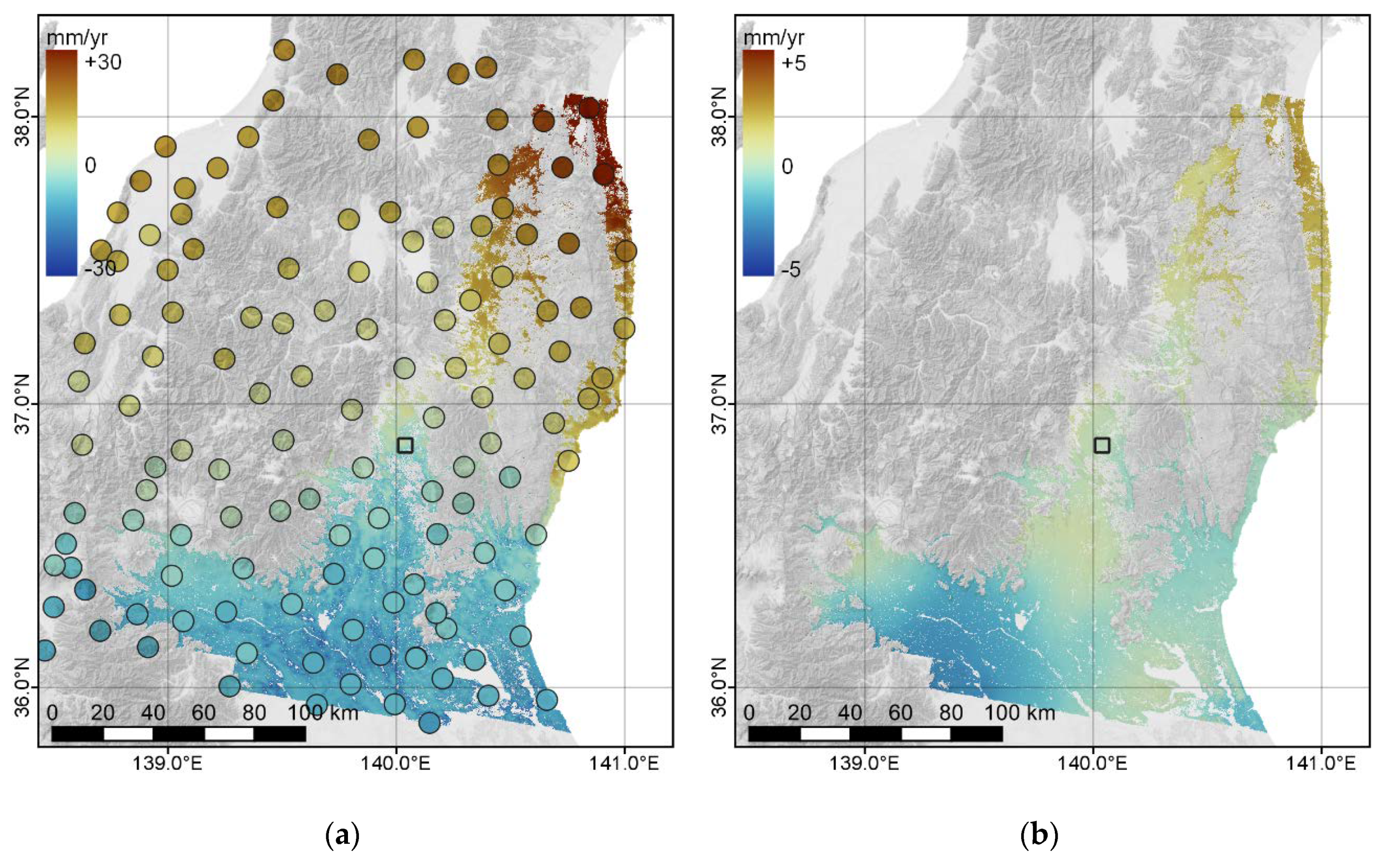
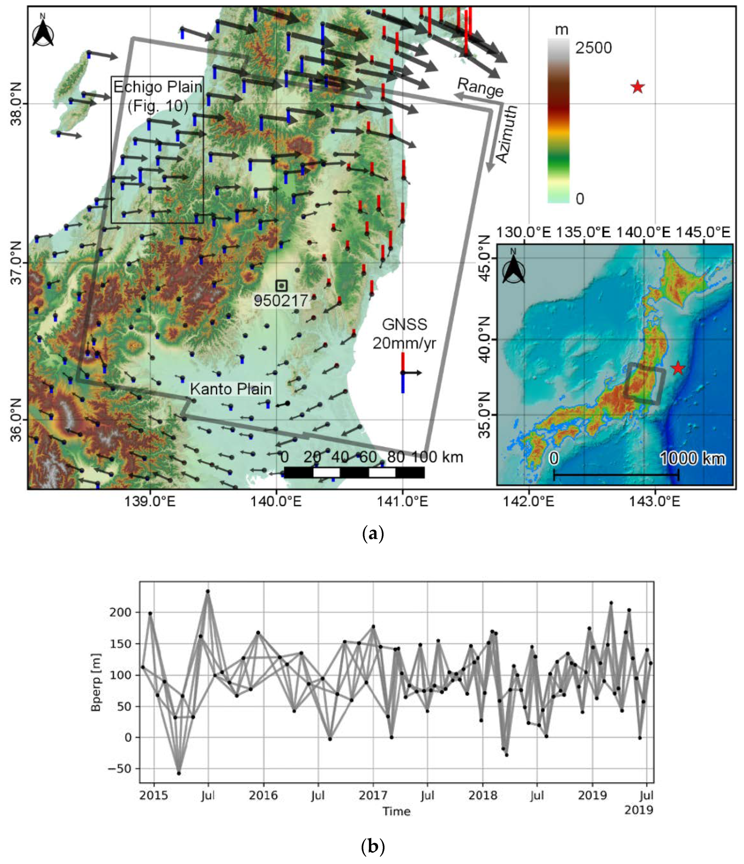
3.1. Southern Tohoku, Japan
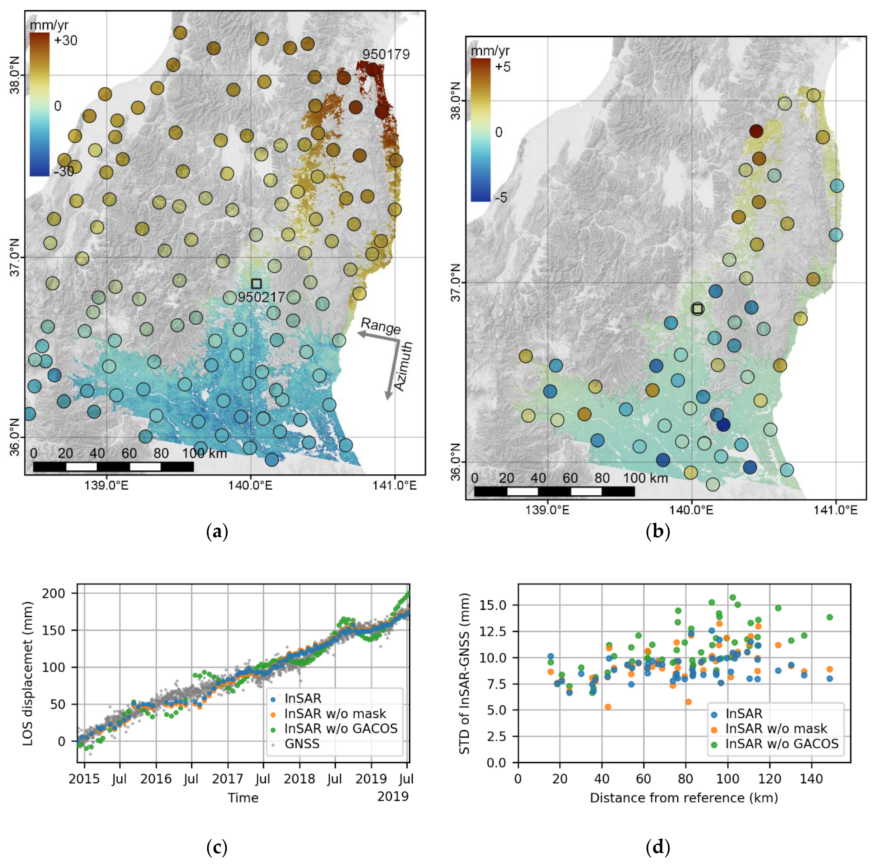
3.2. Results
3.3. Impact of Masking and a Network Gap
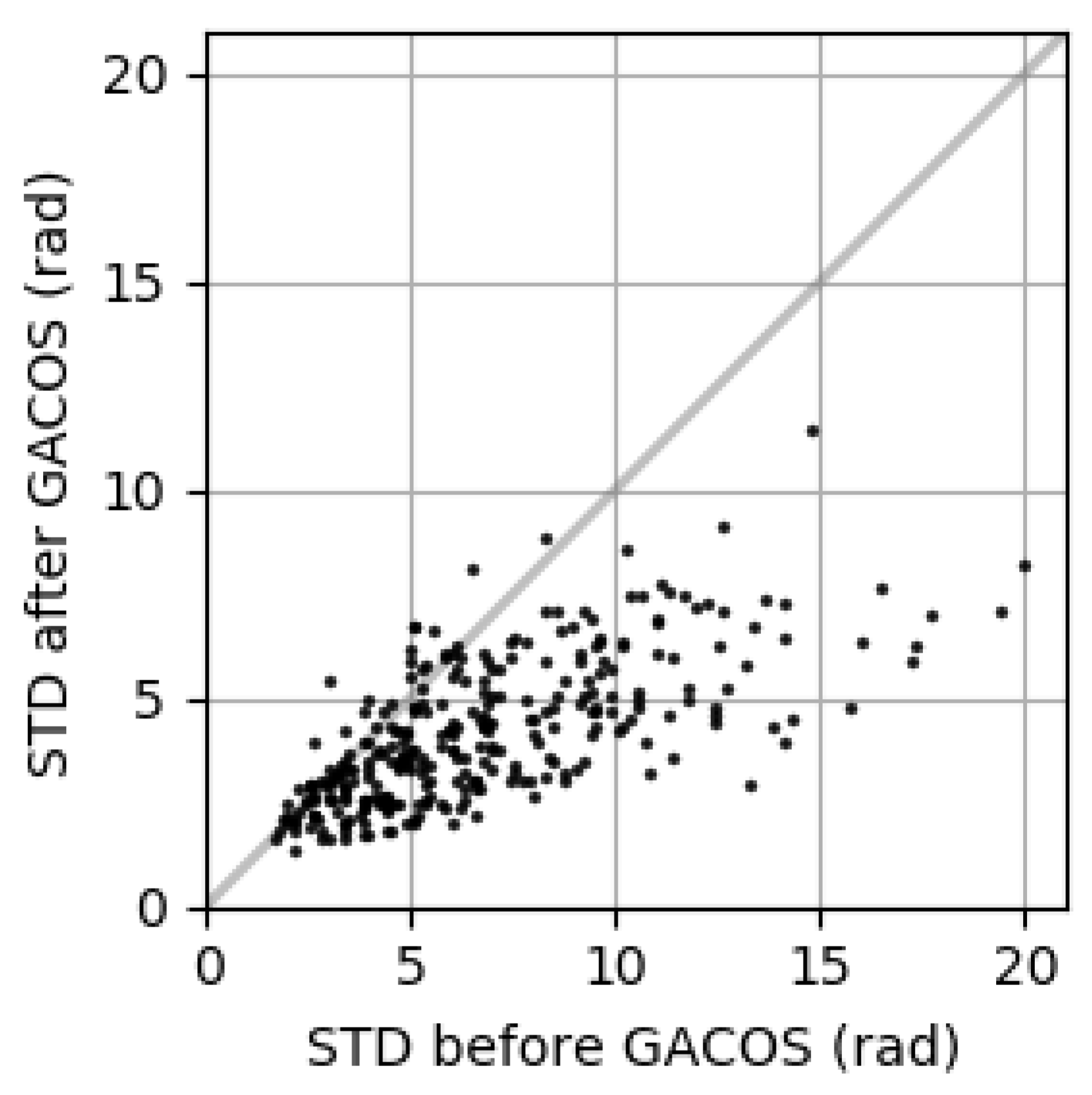
3.4. Impact of the GACOS Correction
3.5. Evolution of Velocity Uncertainty
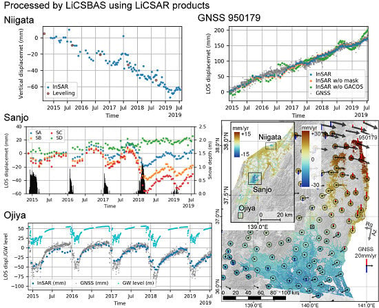
4. Case Study: Clipped Area
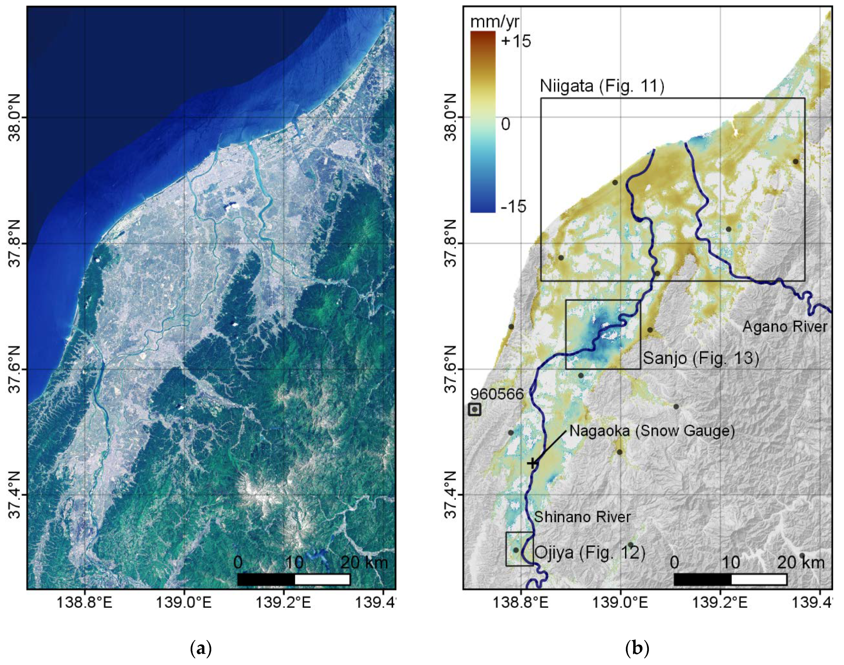
4.1. Echigo Plain
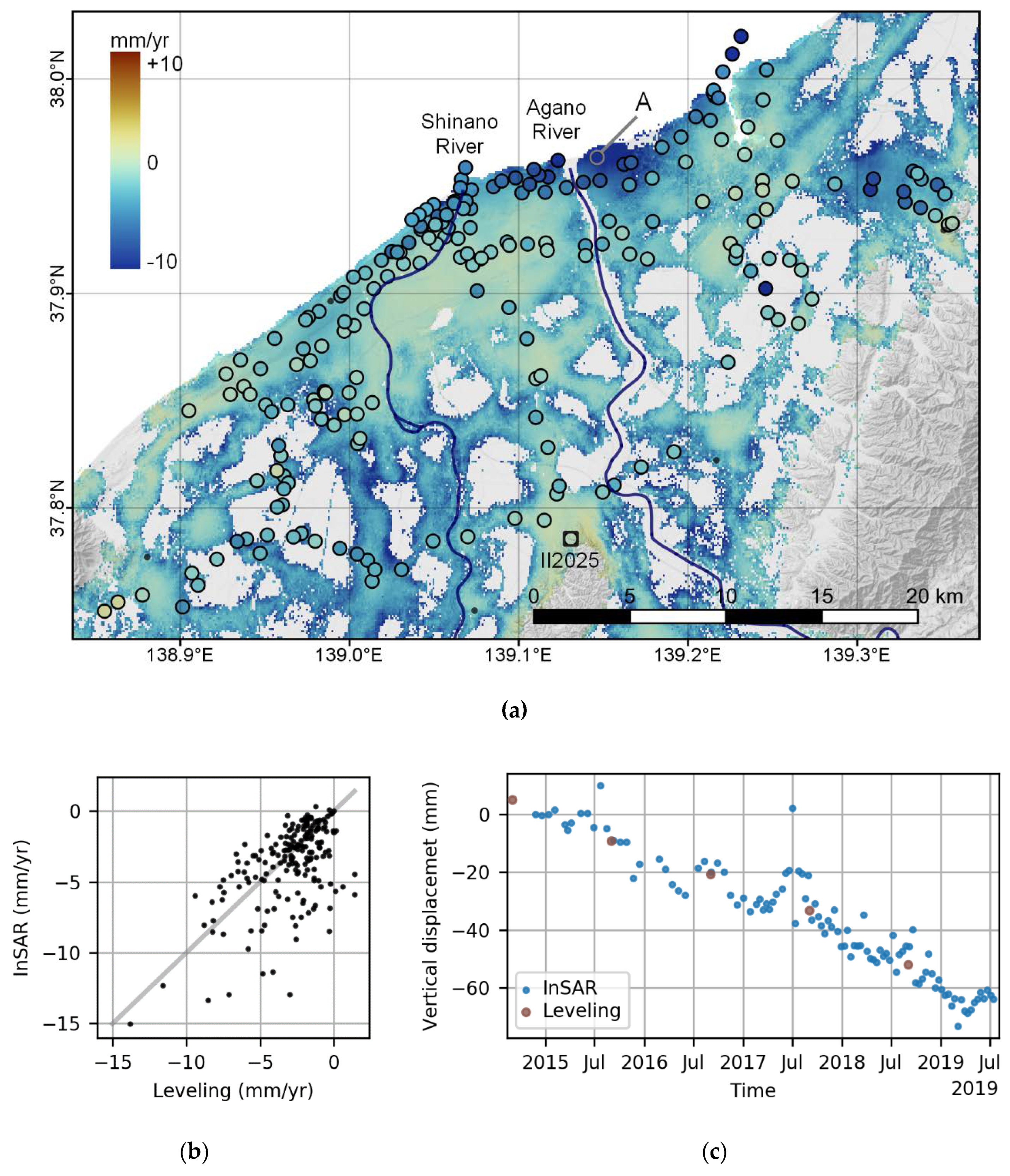
4.2. Niigata City
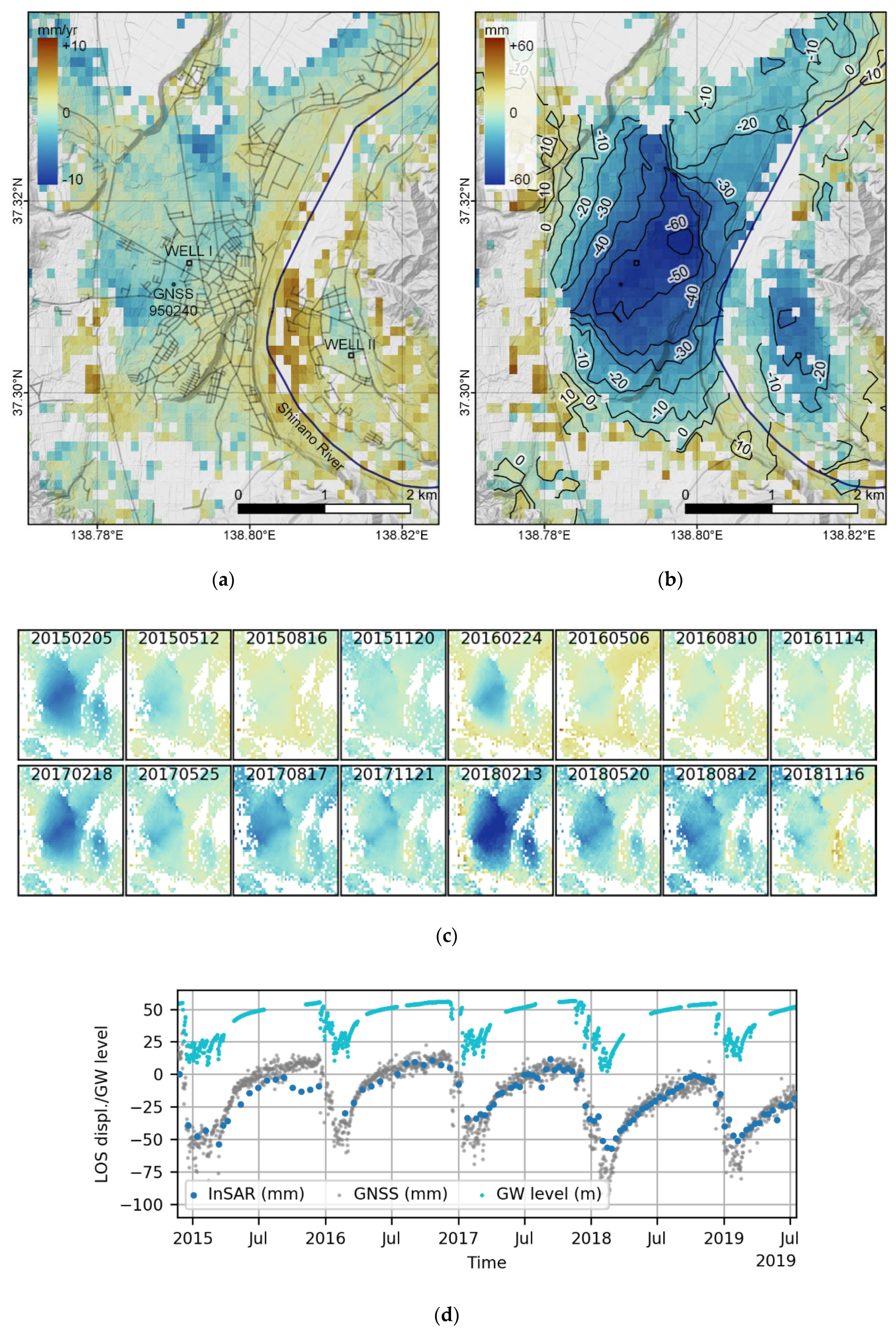
4.3. Ojiya City
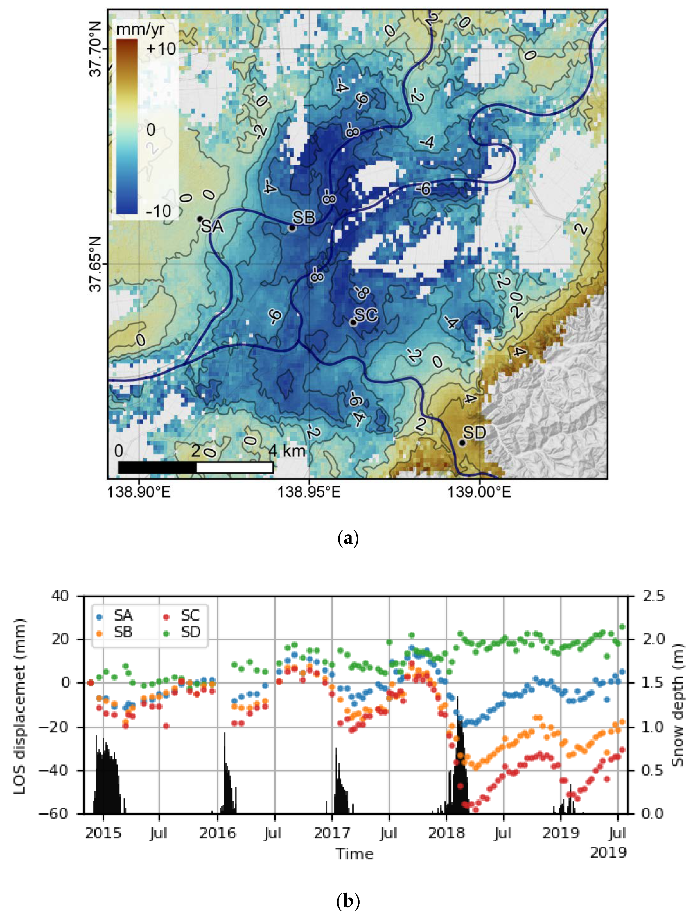
4.4. Sanjo City
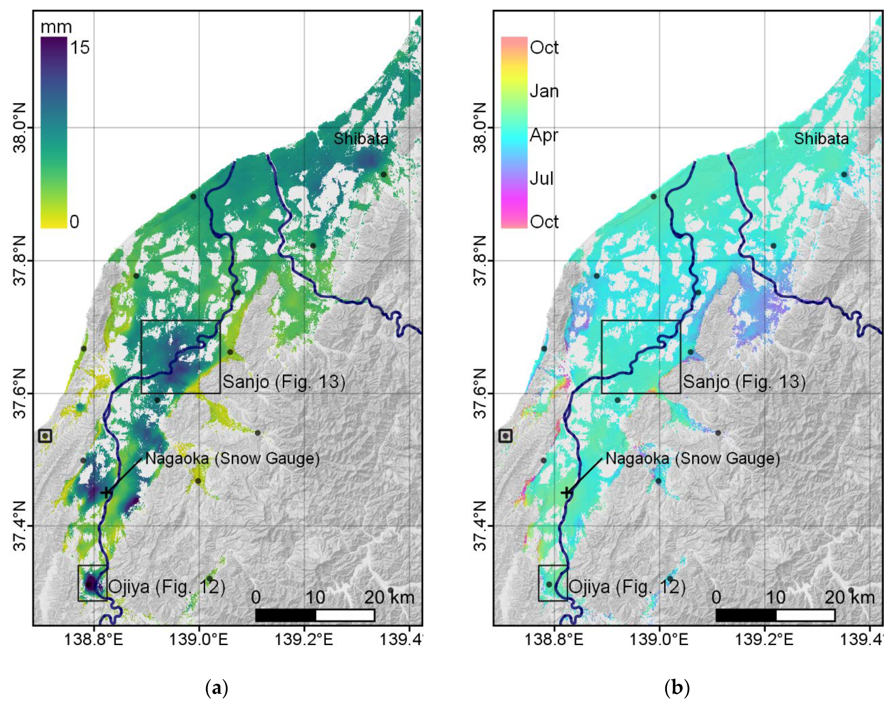
4.5. Annual Displacement in Echigo Plain
5. Discussion
5.1. Processing Time and Disk Usage
5.2. Limitations
6. Conclusions
Supplementary Materials
Author Contributions
Funding
Acknowledgments
Conflicts of Interest
References
- Zhou, X.; Chang, N.-B.; Li, S. Applications of SAR Interferometry in Earth and Environmental Science Research. Sensors 2009, 9, 1876–1912. [Google Scholar] [CrossRef] [Green Version]
- Elliott, J.R.; Walters, R.J.; Wright, T.J. The role of space-based observation in understanding and responding to active tectonics and earthquakes. Nat. Commun. 2016, 7, 13844. [Google Scholar] [CrossRef] [Green Version]
- Hooper, A.J.; Bekaert, D.; Spaans, K.; Arikan, M. Recent advances in SAR interferometry time series analysis for measuring crustal deformation. Tectonophysics 2012, 514–517, 1–13. [Google Scholar] [CrossRef]
- Osmanoğlu, B.; Sunar, F.; Wdowinski, S.; Cabral-Cano, E. Time series analysis of InSAR data: Methods and trends. ISPRS J. Photogramm. Remote Sens. 2016, 115, 90–102. [Google Scholar] [CrossRef]
- Ferretti, A.; Prati, C.; Rocca, F. Permanent Scatters in SAR Interferometry. IEEE Trans. Geosci. Remote Sens. 2001, 39, 8–20. [Google Scholar] [CrossRef]
- Hooper, A.; Segall, P.; Zebker, H. Persistent scatterer interferometric synthetic aperture radar for crustal deformation analysis, with application to Volcán Alcedo, Galápagos. J. Geophys. Res. Solid Earth 2007, 112, 1–21. [Google Scholar] [CrossRef] [Green Version]
- Berardino, P.; Fornaro, G.; Lanari, R.; Sansosti, E. A new algorithm for surface deformation monitoring based on small baseline differential SAR interferograms. IEEE Trans. Geosci. Remote Sens. 2002, 40, 2375–2383. [Google Scholar] [CrossRef] [Green Version]
- Ferretti, A.; Fumagalli, A.; Novali, F.; Prati, C.; Rocca, F.; Rucci, A. A new algorithm for processing interferometric data-stacks: SqueeSAR. IEEE Trans. Geosci. Remote Sens. 2011, 49, 3460–3470. [Google Scholar] [CrossRef]
- Tong, X.; Sandwell, D.T.; Smith-Konter, B. High-resolution interseismic velocity data along the San Andreas Fault from GPS and InSAR. J. Geophys. Res. Solid Earth 2013, 118, 369–389. [Google Scholar] [CrossRef] [Green Version]
- Hussain, E.; Wright, T.J.; Walters, R.J.; Bekaert, D.P.S.; Lloyd, R.; Hooper, A. Constant strain accumulation rate between major earthquakes on the North Anatolian Fault. Nat. Commun. 2018, 9, 1392. [Google Scholar] [CrossRef]
- Homepage | Copernicus. Available online: https://www.copernicus.eu/en (accessed on 27 November 2019).
- Potin, P.; Rosich, B.; Miranda, N.; Grimont, P.; Shurmer, I.; O’Connell, A.; Krassenburg, M.; Gratadour, J.-B. Copernicus Sentinel-1 Constellation Mission Operations Status. In Proceedings of the IGARSS 2019—2019 IEEE International Geoscience and Remote Sensing Symposium; IEEE: Yokohama, Japan, 2019; pp. 5385–5388. [Google Scholar] [CrossRef]
- Sandwell, D.; Mellors, R.; Tong, X.; Wei, M.; Wessel, P. Open radar interferometry software for mapping surface Deformation. Eos Trans. Am. Geophys. Union 2011, 92, 234. [Google Scholar] [CrossRef] [Green Version]
- gmtsar: GMTSAR. Available online: https://github.com/gmtsar/gmtsar (accessed on 27 November 2019).
- Rosen, P.A.; Gurrola, E.; Sacco, G.F.; Zebker, H. The InSAR scientific computing environment. In Proceedings of the IEEE EUSAR 2012 9th European Conference on Synthetic Aperture Radar, Nuremberg, Germany, 23–26 April 2012. [Google Scholar]
- isce2: InSAR Scientific Computing Environment Version 2. Available online: https://github.com/isce-framework/isce2 (accessed on 27 November 2019).
- STEP | Science Toolbox Exploitation Platform. Available online: http://step.esa.int/main/ (accessed on 27 November 2019).
- Agram, P.S.; Jolivet, R.; Riel, B.; Lin, Y.N.; Simons, M.; Hetland, E.; Doin, M.-P.; Lasserre, C. New Radar Interferometric Time Series Analysis Toolbox Released. Eos Trans. Am. Geophys. Union 2013, 94, 69–70. [Google Scholar] [CrossRef] [Green Version]
- Agram, P.; Jolivet, R.; Simons, M. Generic InSAR Analysis Toolbox (GIAnT)—User Guide. Available online: http://earthdef.caltech.edu (accessed on 27 November 2019).
- MintPy: Miami InSAR Time-Series Software in Python. Available online: https://github.com/insarlab/MintPy (accessed on 27 November 2019).
- Yunjun, Z.; Fattahi, H.; Amelung, F. Small baseline InSAR time series analysis: Unwrapping error correction and noise reduction. Comput. Geosci. 2019, 133, 104331. [Google Scholar] [CrossRef] [Green Version]
- StaMPS: Stanford Method for Persistent Scatterers. Available online: https://github.com/dbekaert/StaMPS (accessed on 27 November 2019).
- Galve, J.; Pérez-Peña, J.; Azañón, J.; Closson, D.; Caló, F.; Reyes-Carmona, C.; Jabaloy, A.; Ruano, P.; Mateos, R.; Notti, D.; et al. Evaluation of the SBAS InSAR Service of the European Space Agency’s Geohazard Exploitation Platform (GEP). Remote Sens. 2017, 9, 1291. [Google Scholar] [CrossRef] [Green Version]
- Cignetti, M.; Manconi, A.; Manunta, M.; Giordan, D.; De Luca, C.; Allasia, P.; Ardizzone, F. Taking Advantage of the ESA G-POD Service to Study Ground Deformation Processes in High Mountain Areas: A Valle d’Aosta Case Study, Northern Italy. Remote Sens. 2016, 8, 852. [Google Scholar] [CrossRef] [Green Version]
- ARIA Products. Available online: https://aria-products.jpl.nasa.gov/ (accessed on 27 November 2019).
- Bekaert, D.; Karim, M.; Justin, L.; Hua, H.; Agram, P.; Owen, S.; Manipon, G.; Malarout, N.; Lucas, M.; Sacco, G.; et al. Development and Dissemination of Standardized Geodetic Products by the Advanced Rapid Imaging and Analysis (ARIA) Center for Natural Hazards. In Proceedings of the International Union of Geodesy and Geophysics (IUGG), Montreal, Canada, 8–18 July 2019. [Google Scholar]
- ARIA-Tools: Tools for Exploiting ARIA Standard Products. Available online: https://github.com/aria-tools/ARIA-tools (accessed on 27 November 2019).
- Wegmüller, U.; Werner, C.; Strozzi, T.; Wiesmann, A.; Frey, O.; Santoro, M. Sentinel-1 Support in the GAMMA Software. Procedia Comput. Sci. 2016, 100, 1305–1312. [Google Scholar] [CrossRef] [Green Version]
- Werner, C.; Wegmüller, U.; Strozzi, T.; Wiesmann, A. GAMMA SAR and interferometric processing software. In Proceedings of the ERS-Envisat Symposium, Gothenburg, Sweden, 16–20 October 2000. [Google Scholar]
- COMET-LiCS Sentinel-1 InSAR Portal. Available online: https://comet.nerc.ac.uk/COMET-LiCS-portal/ (accessed on 27 November 2019).
- LiCSBAS: LiCSBAS Package to Conduct InSAR Time Series Analysis Using LiCSAR Products. Available online: https://github.com/yumorishita/LiCSBAS (accessed on 27 November 2019).
- Scheiber, R.; Moreira, A. Coregistration of interferometric SAR images using spectral diversity. IEEE Trans. Geosci. Remote Sens. 2000, 38, 2179–2191. [Google Scholar] [CrossRef]
- Prats-Iraola, P.; Scheiber, R.; Marotti, L.; Wollstadt, S.; Reigber, A. TOPS Interferometry With TerraSAR-X. IEEE Trans. Geosci. Remote Sens. 2012, 50, 3179–3188. [Google Scholar] [CrossRef] [Green Version]
- Goldstein, R.M.; Werner, C.L. Radar interferogram filtering for geophysical applications. Geophys. Res. Lett. 1998, 25, 4035–4038. [Google Scholar] [CrossRef] [Green Version]
- Hooper, A.J. A statistical-cost approach to unwrapping the phase of InSAR time series. In Proceedings of the Fringe 2009 Workshop, Frascati, Italy, 30 November–4 December 2009. [Google Scholar]
- Chen, C.W.; Zebker, H.A. Phase unwrapping for large SAR interferograms: Statistical segmentation and generalized network models. IEEE Trans. Geosci. Remote Sens. 2002, 40, 1709–1719. [Google Scholar] [CrossRef] [Green Version]
- Lazecky, M.; Maghsoudi, Y.; Morishita, Y.; Wright, T.J.; Hooper, A.; Elliott, J.; Hatton, E.; Greenall, N.; Gonzalez, P.J.; Spaans, K.; et al. LiCSAR: An Automatic InSAR Tool for Measuring and Monitoring Tectonic and Volcanic Activities. Manuscript in Preparation.
- Yu, C.; Li, Z.; Penna, N.T.; Crippa, P. Generic Atmospheric Correction Model for Interferometric Synthetic Aperture Radar Observations. J. Geophys. Res. Solid Earth 2018, 123, 9202–9222. [Google Scholar] [CrossRef]
- Hanssen, R.F. Radar Interferometry; Remote Sensing and Digital Image Processing; Springer: Dordrecht, The Netherlands, 2001; Volume 2, ISBN 978-0-7923-6945-5. [Google Scholar]
- Bekaert, D.P.S.; Walters, R.J.; Wright, T.J.; Hooper, A.J.; Parker, D.J. Statistical comparison of InSAR tropospheric correction techniques. Remote Sens. Environ. 2015, 170, 40–47. [Google Scholar] [CrossRef] [Green Version]
- Hamlyn, J.; Wright, T.; Walters, R.; Pagli, C.; Sansosti, E.; Casu, F.; Pepe, S.; Edmonds, M.; McCormick Kilbride, B.; Keir, D.; et al. What causes subsidence following the 2011 eruption at Nabro (Eritrea)? Prog. Earth Planet. Sci. 2018, 5, 31. [Google Scholar] [CrossRef] [Green Version]
- Jung, J.; Kim, D.J.; Park, S.E. Correction of atmospheric phase screen in time series InSAR using WRF model for monitoring volcanic activities. IEEE Trans. Geosci. Remote Sens. 2014, 52, 2678–2689. [Google Scholar] [CrossRef]
- Morishita, Y.; Kobayashi, T. Ground Surface Displacement of Kirishima Volcano Group Detected by ALOS-2 InSAR Time Series Analysis and Effect of Atmospheric Noise Reduction. J. Geod. Soc. Japan 2018, 64, 28–38. [Google Scholar] [CrossRef]
- Set I - Atmospheric Model High Resolution 10-Day Forecast (HRES) | ECMWF. Available online: https://www.ecmwf.int/en/forecasts/datasets/set-i (accessed on 27 November 2019).
- GACOS. Available online: http://ceg-research.ncl.ac.uk/v2/gacos/ (accessed on 27 November 2019).
- Wang, Q.; Yu, W.; Xu, B.; Wei, G. Assessing the Use of GACOS Products for SBAS-InSAR Deformation Monitoring: A Case in Southern California. Sensors 2019, 19, 3894. [Google Scholar] [CrossRef]
- Wang, X.; Aoki, Y.; Chen, J. Surface deformation of Asama volcano, Japan, detected by time series InSAR combining persistent and distributed scatterers, 2014‒2018. Earth Planets Space 2019, 71, 121. [Google Scholar] [CrossRef]
- Shen, L.; Hooper, A.; Elliott, J. A Spatially Varying Scaling Method for InSAR Tropospheric Corrections Using a High-Resolution Weather Model. J. Geophys. Res. Solid Earth 2019, 124, 4051–4068. [Google Scholar] [CrossRef] [Green Version]
- Biggs, J.; Wright, T.; Lu, Z.; Parsons, B. Multi-interferogram method for measuring interseismic deformation: Denali Fault, Alaska. Geophys. J. Int. 2007, 170, 1165–1179. [Google Scholar] [CrossRef] [Green Version]
- López-Quiroz, P.; Doin, M.P.; Tupin, F.; Briole, P.; Nicolas, J.M. Time series analysis of Mexico City subsidence constrained by radar interferometry. J. Appl. Geophys. 2009, 69, 1–15. [Google Scholar] [CrossRef]
- De Zan, F.; Zonno, M.; Lopez-Dekker, P. Phase Inconsistencies and Multiple Scattering in SAR Interferometry. IEEE Trans. Geosci. Remote Sens. 2015, 53, 6608–6616. [Google Scholar] [CrossRef] [Green Version]
- Schmidt, D.A.; Bürgmann, R. Time-dependent land uplift and subsidence in the Santa Clara valley, California, from a large interferometric synthetic aperture radar data set. J. Geophys. Res. Solid Earth 2003, 108, 1–13. [Google Scholar] [CrossRef] [Green Version]
- Doin, M.-P.; Lodge, F.; Guillaso, S.; Jolivet, R.; Lasserre, C.; Ducret, G.; Grandin, R.; Pathier, E.; Pinel, V. Presentation of the small baseline NSBAS processing chain on a case example: The Etna deformation monitoring from 2003 to 2010 using Envisat data. In Proceedings of the Fringe 2011 Workshop, Frascati, Italy, 19–23 September 2011. [Google Scholar]
- Efron, B.; Tibshirani, R. Bootstrap Methods for Standard Errors, Confidence Intervals, and Other Measures of Statistical Accuracy. Stat. Sci. 1986, 1, 54–75. [Google Scholar] [CrossRef]
- Hanssen, R.F.; van Leijen, F.J.; van Zwieten, G.J.; Bremmer, C.; Dortland, S.; Kleuskens, M. Validation of existing processing chains in TerraFirma stage 2. Product validation: Validation in the Amsterdam and Alkmaar area Draft version 3. 2008. Available online: https://raw.githubusercontent.com/wiki/yumorishita/LiCSBAS/documents/Hanssen_2008.pdf (accessed on 27 January 2020).
- Hoffmann, J.; Zebker, H.A.; Galloway, D.L.; Amelung, F. Seasonal subsidence and rebound in Las Vegas Valley, Nevada, observed by synthetic aperture radar interferometry. Water Resour. Res. 2001, 37, 1551–1566. [Google Scholar] [CrossRef]
- Bell, J.W.; Amelung, F.; Ferretti, A.; Bianchi, M.; Novali, F. Permanent scatterer InSAR reveals seasonal and long-term aquifer-system response to groundwater pumping and artificial recharge. Water Resour. Res. 2008, 44. [Google Scholar] [CrossRef] [Green Version]
- Ozawa, S.; Nishimura, T.; Suito, H.; Kobayashi, T.; Tobita, M.; Imakiire, T. Coseismic and postseismic slip of the 2011 magnitude-9 Tohoku-Oki earthquake. Nature 2011, 475, 373–376. [Google Scholar] [CrossRef]
- Suito, H. Current Status of Postseismic Deformation Following the 2011 Tohoku-Oki Earthquake. J. Disaster Res. 2018, 13, 503–510. [Google Scholar] [CrossRef]
- Geospatial Information Authority of Japan. Crustal Movements in the Tohoku District. Rep. Coord. Comm. Earthq. Predict. 2018, 100, 56–68. [Google Scholar]
- Liang, C.; Agram, P.; Simons, M.; Fielding, E.J. Ionospheric Correction of InSAR Time Series Analysis of C-band Sentinel-1 TOPS Data. IEEE Trans. Geosci. Remote Sens. 2019, 57, 6755–6773. [Google Scholar] [CrossRef] [Green Version]
- Weiss, J.R.; Walters, R.J.; Morishita, Y.; Wright, T.J.; Lazecky, M.; Wang, H.; Hussain, E.; Hooper, A.J.; Elliott, J.R.; González, P.J.; et al. Plate-scale measurements of interseismic velocity and strain from Sentinel-1 InSAR and GNSS data. Manuscript in Preparation.
- Zhang, J.; Bock, Y.; Johnson, H.; Fang, P.; Williams, S.; Genrich, J.; Wdowinski, S.; Behr, J. Southern California permanent GPS geodetic array: Error analysis of daily position estimates and site velocities. J. Geophys. Res. Solid Earth 1997, 102, 18035–18055. [Google Scholar] [CrossRef]
- Aoki, S. Land Sibsidence in Niigata. In Proceedings of the Anaheim Symposium, Anaheim, CA, USA, 13–17 December 1976; pp. 105–112. [Google Scholar]
- Niigata Prefecture Ground Subsidence In the Niigata Plain. Available online: http://npdas.pref.niigata.lg.jp/kankyotaisaku/5c85f40531a5c.pdf (accessed on 27 November 2019).
- Kanto Bureau of International Trade and Industry. Report for Rationalization of Ground Water Use in Ojiya Area in Niigata Prefecture (Edition for Hydrological Analysis); Kanto Bureau of International Trade and Industry: Tokyo, Japan, 1994. [Google Scholar]
- Sato, H.P.; Abe, K.; Ootaki, O. GPS-measured land subsidence in Ojiya City, Niigata Prefecture, Japan. Eng. Geol. 2003, 67, 379–390. [Google Scholar] [CrossRef]
- Chaussard, E.; Bürgmann, R.; Shirzaei, M.; Fielding, E.J.; Baker, B. Predictability of hydraulic head changes and characterization of aquifer-system and fault properties from InSAR-derived ground deformation. J. Geophys. Res. Solid Earth 2014, 119, 6572–6590. [Google Scholar] [CrossRef]
- Morishita, Y.; Hanssen, R.F. Deformation Parameter Estimation in Low Coherence Areas Using a Multisatellite InSAR Approach. IEEE Trans. Geosci. Remote Sens. 2015, 53, 4275–4283. [Google Scholar] [CrossRef]
- Rocca, F. Modeling interferogram stacks. IEEE Trans. Geosci. Remote Sens. 2007, 45, 3289–3299. [Google Scholar] [CrossRef]
- Zebker, H.A.; Villasenor, J. Decorrelation in Inteferometric Radar Echoes. IEEE Trans. Geosci. Remote Sens. 1992, 30, 950–959. [Google Scholar] [CrossRef] [Green Version]
- Morishita, Y.; Hanssen, R.F. Temporal decorrelation in L-, C-, and X-band satellite radar interferometry for pasture on drained peat soils. IEEE Trans. Geosci. Remote Sens. 2015, 53, 1096–1104. [Google Scholar] [CrossRef]


| Noise index | Meaning |
|---|---|
| coh_avg | Average value of the interferometric coherence across the stack (0–1). |
| n_unw | Number of unwrapped data used in the time series calculation. |
| vstd | Standard deviation of the velocity (mm/yr) estimated in Step 1-4. |
| maxTlen | Maximum time length of the connected network (years).The larger the value, the better the precision in the velocity estimate (see Section 3.5). |
| n_gap | Number of gaps in the interferogram network and time series breaks. |
| stc | Spatiotemporal consistency (mm) [55], which is the minimum root mean square (RMS) of the double differences of the time series in space and time between the pixel of interest and an adjacent pixel among all adjacent pixels. |
| n_ifg_noloop | Number of interferograms with no loops that cannot be checked by the loop closure and possibly have unidentified unwrapping errors. |
| n_loop_err | Number of the unclosed loops after the network refinement in Step 1-2. |
| resid_rms | RMS of residuals in the small baseline (SB) inversion (mm). |
| Entire Frame | Echigo Plain | Entire Frame (10 × 10 Downsampled) | |
|---|---|---|---|
| Size of Image | 3338 × 2685 | 732 × 922 | 333 × 268 |
| # of Images | 104 | 104 | 104 |
| # of Interferograms | 306 | 306 | 306 |
| # of Inverted Pixels (at Step 1-3) | 2,503,334 | 288,079 | 24,579 |
| # of Remaining Pixels (after Step 1-6) | 1,166,756 | 167,269 | 15,704 |
| Step 0-1 | 10 min | — | — |
| Step 0-2 | 10 min | — | 3 min |
| Step 0-3 | 30 min | — | 5 min |
| Step 0-4 | 5 min | 2 min | 1 min |
| Step 0-5 | — | 5 min | — |
| Step 1-1 | 2 min | <1 min | <1 min |
| Step 1-2 | 20 min | 4 min | 3 min |
| Step 1-3 | 3 hr 30 min | 25 min | 5 min |
| Step 1-4 | 20 min | 2 min | <1 min |
| Step 1-5 | <1 min | <1 min | <1 min |
| Step 1-6 | 30 min | 5 min | 2 min |
| Total Time for Step 1 | ~5 hr | ~40 min | ~10 min |
| Size of Downloaded GeoTIFF | 5 GB | — | — |
| Size of GACOS Data | 5 GB | — | — |
| Size of Converted Data | 21 GB | 2 GB | 0.2 GB |
| Size of Created Data in Step 1 | 10 GB | 1 GB | 0.2 GB |
© 2020 by the authors. Licensee MDPI, Basel, Switzerland. This article is an open access article distributed under the terms and conditions of the Creative Commons Attribution (CC BY) license (http://creativecommons.org/licenses/by/4.0/).
Share and Cite
Morishita, Y.; Lazecky, M.; Wright, T.J.; Weiss, J.R.; Elliott, J.R.; Hooper, A. LiCSBAS: An Open-Source InSAR Time Series Analysis Package Integrated with the LiCSAR Automated Sentinel-1 InSAR Processor. Remote Sens. 2020, 12, 424. https://doi.org/10.3390/rs12030424
Morishita Y, Lazecky M, Wright TJ, Weiss JR, Elliott JR, Hooper A. LiCSBAS: An Open-Source InSAR Time Series Analysis Package Integrated with the LiCSAR Automated Sentinel-1 InSAR Processor. Remote Sensing. 2020; 12(3):424. https://doi.org/10.3390/rs12030424
Chicago/Turabian StyleMorishita, Yu, Milan Lazecky, Tim J. Wright, Jonathan R. Weiss, John R. Elliott, and Andy Hooper. 2020. "LiCSBAS: An Open-Source InSAR Time Series Analysis Package Integrated with the LiCSAR Automated Sentinel-1 InSAR Processor" Remote Sensing 12, no. 3: 424. https://doi.org/10.3390/rs12030424