Automatic Mapping of Center Line of Railway Tracks using Global Navigation Satellite System, Inertial Measurement Unit and Laser Scanner

Abstract

Up-to-date geodatasets on railway infrastructure are valuable resources for the field of transportation. This paper investigates three methods for mapping the center lines of railway tracks using heterogeneous sensor data: (i) conditional selection of satellite navigation (GNSS) data, (ii) a combination of inertial measurements (IMU data) and GNSS data in a Kalman filtering and smoothing framework and (iii) extraction of center lines from laser scanner data. Several combinations of the methods are compared with a focus on mapping in tree-covered areas. The center lines of the railway tracks are extracted by applying these methods to a test dataset collected by a road-rail vehicle. The guard rails in the test area were also extracted during the center line detection process. The combination of methods (i) and (ii) gave the best result for the track on which the measurement vehicle had moved, mapping almost 100% of the track. The combination of methods (ii) and (iii) and the combination of all three methods gave the best result for the other parallel tracks, mapping between 25% and 80%. The mean perpendicular distance of the mapped center lines from the reference data was 1.49 meters.

1. Introduction

Geodatasets on railway infrastructure are useful resources in the transportation sector for routing applications and planning construction activities [1,2,3]. From the maintenance perspective, it is necessary to periodically examine the infrastructure for defects and damages that might affect the normal operation of trains [2,4,5,6]. Traditionally, the infrastructure is mapped by terrestrial surveys using tachymeters and total stations. Although the employed methods are highly accurate, they are time-consuming and expensive [1,4]. Therefore, research is driven towards algorithms that automatically map the railway infrastructure from data collected using a wide range of sensors such as digital cameras, laser scanners, global navigation satellite system (GNSS) receivers and eddy current sensors (ECS) [1,2,3,4,5,6,7,8]. By following methods based on sensor data, both the cost and time are significantly reduced. This also enables periodical repetition of the mapping process in order to account for changes in the infrastructure [2,4,5,6].

The focus of this study was to map the center line of the tracks with a fully automated approach. Looking at previous studies carried out in this context, some of them used laser scanner data collected from an aerial platform with or without aerial images and developed methods to extract tracks from them [1,2,9,10]. The main benefit of this approach is that it can cover vast areas in a short period of time. However, it is suitable for mapping only those tracks that are visible from an aerial platform. It cannot map tracks in forests or inside tunnels [2]. In order to overcome this drawback, some studies extracted tracks from laser scanner data collected from a mobile terrestrial platform [2,3,4,5,6,7,9]. In most of these studies, the height of the points scanned by the laser scanner was used to identify tracks. Elberink et al. [5] identified railway tracks by analysing the histogram of height values and using the height, linearity and parallelity of rails. Two years later, Elberink and Khoshelham [4] published their work on the automatic extraction of center line of railway tracks from laser scanner data using data-driven and model-driven approaches. Their approach of pairing the lines and generating center lines looks promising. With a focus on laser data analysis, details of positioning the measurement platform are omitted. Zhu and Hyyppa [9] attempted to automatically identify objects that can be found in a railway environment using laser scanner data. However, they did not generate the center lines of the rails they had detected. Arastounia [2,6] calculated the standard deviation of the height of the points in the track bed and analysed the histogram of standard deviation to identify rails. They clustered points that were close and joined line segments that were close and were oriented in the same direction. Laser scanners also measure the energy of the received laser pulses. Yang and Feng [3] identified railway tracks using knowledge of the shape of rails and these energy values. They used a moving window and calculated the difference in height of the points in the window, the slope of the rail and the energy value of points. They observed that the energy values were helpful in differentiating rails from the surrounding ballast and sleepers.

The trajectory of a moving platform can be observed using a GNSS receiver [11]. A GNSS receiver on a rail vehicle can provide information about the center line of the track given its antenna is placed appropriately. Inertial measurement units (IMU) measure vehicle accelerations and turn rates that can be combined with the GNSS data to improve the trajectory estimation. This has been demonstrated in several studies [12,13,14,15,16,17]. Depending on the processed GNSS data, different variants can be distinguished. This paper suggests a loosely coupled GNSS and IMU integration in which the GNSS position and speed output is processed instead of the pseudo-ranges of all visible satellites [11]. Most approaches rely on Kalman filters and related algorithms [18,19,20] as data fusion method. For post-processing applications, Rauch-Tung-Striebel (RTS) smoothing [20] can further improve the results of a Kalman filter. The use of smoothing, albeit a simple extension beyond the Kalman filter fusion of GNSS and IMU data, is seldom described in the literature. In fact, the positioning task is often omitted in the mapping literature, with mere reference to the employed hardware [4,5,6]. We believe that our contribution which provides insights into the Kalman filtering methodology and the potential of smoothing are beneficial for the mapping audience and show how the approaches can enhance the mapping process. After all, without having an accurate position of the measurement platform, errors carry over to the analysis of laser data to find parallel tracks. Specifically, the influence of the quality of GNSS data on Kalman filters is examined in tree-covered areas and areas with unobstructed view from the GNSS receiver to the satellites.

The goal of this work is to compare the performance of six approaches to map the center line of railway tracks. The following steps were carried out:

• A rule-set based on available literature to identify GNSS observations of good quality was developed.
• A Kalman filter framework to combine GNSS and IMU measurements was developed.
• An algorithm to identify rails and generate center lines from laser scanner data was developed.
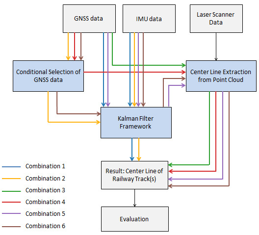
• Center lines were generated from a test dataset using six different combinations of (1), (2) and (3).
• The results were compared and evaluated using center lines digitised from freely available aerial images.

The paper is organised as follows: The methods are described in detail in Section 2, the results and discussion in Section 3 and the conclusions in Section 4.

2. Methodology

Figure 1 summarises the six approaches that were investigated in this study. These six approaches are combinations of three methods. In the first combination, the data collected by the GNSS receiver and IMU were given as input to a data fusion algorithm based on Kalman filtering and smoothing, which generated the trajectory of the vehicle that represents the center line of the driven track. In the second combination, instead of giving all GNSS points to the Kalman filter, only GNSS points of good quality were given, as points of low quality were disregarded based on a set of conditional rules. These variants do only map the driven tracks and cannot recover parallel tracks. In the third and fourth combinations, center lines were detected from georeferenced laser scanner point clouds, using all GNSS observations (combination 3) or the selection of GNSS observations (combination 4). In the fifth and sixth combinations, GNSS and IMU measurements were combined in the Kalman filter framework and the results were used to georeference the laser point cloud. Similar to the previous case, the two combinations varied in the GNSS observations given as input to the algorithm. It should be noted that combinations 3 to 6 also recover tracks parallel to the driven track. The three methods in the workflow (conditional selection of GNSS data, the Kalman filter framework, center line extraction from point clouds) are explained in the respective Section 2.2, Section 2.3 and Section 2.4. The dataset used to test the approaches is described in Section 2.1. The reference data and procedure used to evaluate the results is described in Section 2.5.

2.1. Dataset Description

The Railway Driving and Validation Environment (RailDriVE) [21] is a measurement vehicle of the Deutsches Zentrum für Luft- und Raumfahrt (German Aerospace Center; DLR) Institute of Transportation Systems. The RailDriVE was driven ten times (each of these is henceforth called a run) along different sections of a track in the Ore Mountain Range (Erzgebirge) near Chemnitz, Germany from 2nd to 4th May 2016. The data were collected by a JAVAD Sigma GNSS receiver, an XSens MTi-G inertial measurement unit and a SICK LMS5009 laser scanner. The GNSS receiver used signals from the Global Positioning System (GPS) and the Global Orbiting Navigation Satellite System (GLONASS). The data collection rate of the sensors was 10 Hz for the GNSS, 100 Hz for the IMU and 25 Hz for the laser scanner. The laser scanner was mounted at a height of 1.4 meters (from the track bed) and tilted 38° towards the ground and so it could cover up to two parallel tracks on either side. The length, duration and the weather condition during data collection are listed in

Table 1. Data acquisition details.

Date	Run	Length (in km)	Duration (in Minutes)	Weather Condition
2 May 2016	1	21.573	92.60	sunny
	2	24.214	83.42
3 May 2016	3	21.628	88.84	sunny
	4	23.601	80.86
	5	23.818	80.86
	6	23.898	92.72
	7	16.611	48.21
	8	14.558	50.99
4 May 2016	9	21.634	68.65	rainy
	10	24.243	89.54	cloudy

.

2.2. Conditional Selection of GNSS Data

The JAVAD Sigma GNSS receiver stored the data as National Marine Electronics Association (NMEA) Sentences (https://www.gpsinformation.org/dale/nmea.htm).

Table 2. Information extracted from National Marine Electronics Association (NMEA) Sentences.

Sentence	Information Extracted
GGA	Latitude, Longitude, Altitude, Number of Satellites observed
GSA	PDOP, HDOP, VDOP
GST	Latitude error, Longitude error, Altitude error
VTG	Speed
HDT	Heading
GMP	Projection, Zone, X and Y value in Projected Coordinate System
GPGSV	Number of GPS satellites observed
GLGSV	Number of GLONASS satellites observed

shows the information that were extracted from these sentences. All entries without positional information were removed. Entries for which projected coordinates in Universal Transverse Mercator (UTM) coordinate system were missing were calculated from latitude and longitude values. Points collected when the vehicle was stationary (speed less than 2 km/h), henceforth called as standstill data, were stored separately.

For the combinations with conditional selection of GNSS data (2, 4, 6), the following rules were chosen from literature and applied on the dataset:

• Number of Satellites >= 4: Theoretically, the GNSS receiver needs at least four satellites to calculate the position [11,22,23,24]. This requirement is not satisfied in areas where there are fewer or no visible satellites and might lead to erroneous observations. Hence, observations made when the number of satellites is less than 4 are considered unreliable [22]. However, most of the modern receivers provide an estimate based on the previous positions when this requirement is not fulfilled. This estimate depends greatly on the quality of the previous observations and the time of the last signal receptions. Hence, all observations made when the number of visible satellites was less than 4 were discarded.
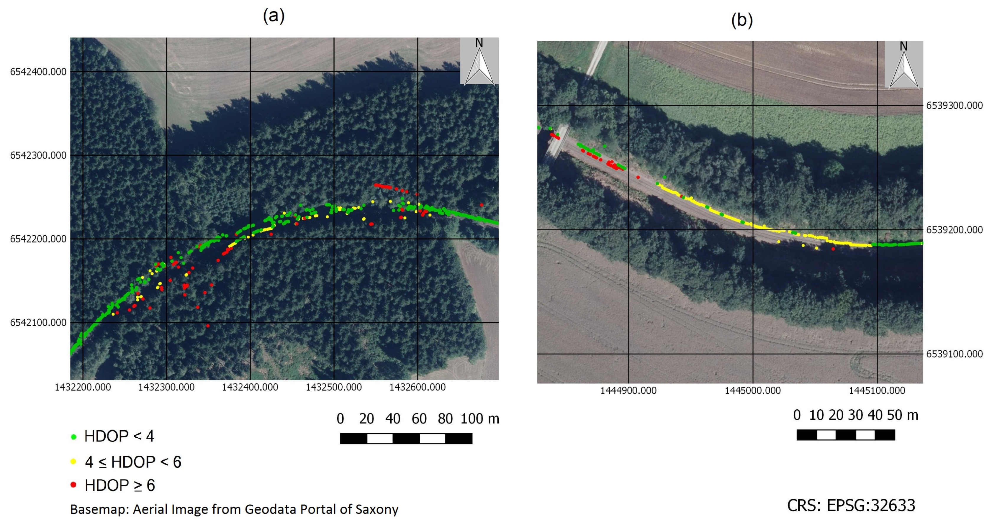
• HDOP < 6: The GNSS receiver records the Dilution of Precision (DOP), which has been widely used to determine the quality of the measurement [22,25]. Several components of DOP exist, such as Horizontal Dilution of Precision (HDOP), Vertical Dilution of Precision (VDOP), Positional Dilution of Precision (PDOP) and Time Dilution of Precision (TDOP) [11]. The components measured depend on the configuration of the GNSS receiver. The value of DOP depends on the geometry of the observed satellites with respect to the receiver. DOP values are smaller when the satellites are well-spread out in the sky and larger when they are clustered [11,22]. Carstensen Jr. [22] suggests the use of points with HDOP less than 4 for precise mapping applications, while Langley [23] suggests 6 as the cutoff value. In this study, both options were tested. Based on the results of these tests (see Appendix A.1), an HDOP value of 6 was chosen as the cutoff value.
• Difference between computed and true speed within a threshold: The GNSS receiver also measures the speed of the measurement platform. If the receiver calculates the speed using Doppler measurements, then these values are highly reliable [26]. When the estimated GNSS speed is accurate, it is possible to identify points that are likely to exhibit large position errors. When the difference between the speed calculated from successive GNSS observations and the true speed is large, then the position of the point can be considered erroneous and omitted from further processing. The point can also be discarded if the speed and acceleration values calculated from positions are unrealistic for that measurement platform [22]. The speed can be calculated from the positions if the time at which the position was measured is known.
  Let $(x_1,y_1)$ and $(x_2,y_2)$ be the positions of the measurement platform at time $t_1$ and $t_2$ respectively. An estimate of the speed s of the platform is calculated as

  $$s=\frac{\sqrt{{(x_2-x_1)}^2+{(y_2-y_1)}^2}}{t_2-t_1}.$$

  (1)
  If $\widehat{s}$ is the speed calculated from Doppler measurements, then,

  $$|s-\widehat{s}|<S,$$

  (2)

  where S is the maximum allowable difference in speed. S value was set to 2 km/h, the reason for which can be found in Appendix A.2.

The three rules, together called the combined rule, were applied to the data collected in the 10 runs. The set of points passing all the three rules were used for the combinations 2, 4 and 6.

2.3. A Kalman Filter Framework to Combine GNSS and IMU Data

Kalman filters are algorithms that can estimate the time-varying state of a dynamical system from an incoming sequence of noise-corrupted measurements [12,13,18,19,20]. Here, the term state refers to a vector that comprises the quantities of interest, namely the position and velocity of the rail vehicle or measurement platform. The evolution of the state vector is described by a motion model in the form of a stochastic state difference equation. The relations between the state vector and the measurements are provided by stochastic measurement equations. The origin of the Kalman filter is in online applications in which the latest state is estimated for discrete times at a fixed and user-determined sampling rate. For post-processing applications such as the mapping based on previously collected batches of sensor data, the Kalman filter results can be further improved using Rauch-Tung-Striebel smoothing [18,20].

For the application at hand, four parameters were chosen as state components: the position $(x,y)$ of the measurement platform in UTM coordinates, the speed (s) of the measurement platform in $m/s$ and the heading angle (h) in radians. So, the state vector is ${\left[xysh\right]}^T$. Only the horizontal position and velocity is included so as to reduce the number of unknowns to be estimated and thereby reduce the estimation errors. The GNSS device provides measurements of all state components at a frequency of 10 Hz, with the position internally computed from pseudo-ranges between the measurement platform and the satellites in view and the speed derived from the Doppler shift in the satellite carrier waves [11]. The heading measurements are internally computed and not measured directly, in contrast. The IMU device provides acceleration and turn rate measurements at a rate of 100 Hz. In the employed filtering solution, only the longitudinal acceleration and the turn rate about the vertical axis are processed. These quantities can be interpreted as temporal derivatives of the state components s and h. The IMU measurements are used as known, yet noise-corrupted inputs to a Kalman filter.

Using a simplified motion model [19] and the measurement relations, as well as information about the sensor uncertainties from the respective data sheets, a Kalman filter was implemented. Because the motion model for the chosen state vector does exhibit some mildly non-linear relations, an extended Kalman filter (EKF) was used. Information about vehicle standstill was employed to separate the estimation tasks into logical units between vehicle start and stops. As a consequence, the vehicle velocity could not change sign in each of these journeys. Standstill data was furthermore used to perform IMU bias calibration and to gain insights about the GNSS error variances. The separate bias estimation in standstill was found to be the simplest and most effective solution for the employed sensor set-up. The sampling rate of the Kalman filter was determined by the IMU input rate and set to 100 Hz. The algorithm itself consists of the iterative update equations for an estimate of the state vector and its covariance. At all time steps of the Kalman filter rate, so called time updates are performed that incorporate the IMU data to propagate the state estimate and its covariance. For time steps with available GNSS measurements, so called measurement updates are performed to correct the state estimate and its covariance in a systematic way. Interested readers are referred to References [18,20] for algorithmic details and the underlying theory of Bayesian state estimation and to Reference [19] for many practical application examples.

Given a good model of the state evolution, in this case a stochastic difference equation that describes the vehicle motion well, the estimation results of a Kalman filter can be improved in an offline setting. The Rauch-Tung-Striebel (RTS) smoother and its variants [18,20] consist of a recursion that runs backwards in time to further process the state estimates and covariance matrices provided by the Kalman filter time and measurement updates. Smoothing is one systematic way to apply batch estimation in a Kalman filtering framework, that is, to estimate the state for all times of interest based on the entire batch of GNSS and IMU data. Albeit a simple algorithm with great potential for improvements over online Kalman filters, RTS smoothing has not been investigated in the related approaches.

The equations used in this work for Kalman filtering and smoothing are given in Appendix B.

Finally, the RTS smoothing position results for the separate periods of motion were re-joined to obtain the complete center line of the driven track.

2.4. Extraction of Center Lines from Georeferenced Point Cloud

The laser scanner on RailDriVE had stored the angle at which the laser pulse was sent (also called the viewing angle), the distance to the object it had hit and the received signal strength indicator (RSSI) for each laser pulse. A 3D point cloud was generated using this information. The 3D point cloud was georeferenced using the raw or conditionally selected GNSS data or the output from the Kalman filter framework depending on the combination.

The terminologies used in the description of the algorithm to extract center lines are shown in Figure 2. The vehicle moves on two pieces of metal called rails. The center line of the track is defined as an imaginary line situated in the middle of the two rails. The distance between the two rails of the track is called the track gauge. In order to provide additional support to the vehicle, there is another piece of metal close to one or both of the rails in some sections of the track. These metal pieces are called guard rails.

The center line of the tracks were extracted from the point cloud using the following steps:

• Identification of laser pulses that hit the rails: Laser pulses that hit the rail would have a higher height value than the surrounding points since the rails are raised above the track bed. They would also have a lower RSSI value than the surrounding because smoother surfaces scatter less energy than rougher surfaces [27]. The plot of height and RSSI values for laser pulses in a single scan is shown in Figure 3. The peaks in the height plot, marked with green circles indicate the rails. At corresponding points in the RSSI plot, there are drops in the value (orange circles). The width of the peaks and the drop in RSSI values was most prominent for the track on which the measurement vehicle was moving. They decreased gradually for other tracks in the area. These peaks and drops were identified using a moving window approach as explained in the next paragraph. If the viewing angle of the laser scanner was between $-{70}^{°}$ to $+{70}^{°}$, points at which both a peak and a drop were found were considered as rails. For other values of viewing angle, all peaks were considered as rails and drops were ignored.
  Firstly, a moving average filter of size 3 measurements (equivalent to a width of 0.5 degrees) was used to reduce noise in the data. A moving window of size 5 measurements (equivalent to 0.833 degrees) was used to identify peaks in the height values. In each position of the moving window, if the center point in the window was the highest point and was 65 to 200 millimeters higher than the mean height in a bigger window of size w, the point was classified as a peak. w value was set to 41 (equivalent to 6.833 degrees) when the viewing angle was between $-{70}^{°}$ and $+{70}^{°}$ and to 21 (equivalent to 3.5 degrees) for other viewing angles. For the RSSI values, a moving window of size 7 (equivalent to 1.167 degrees) was used. A slightly bigger window was used because the drop in energy is more gradual than the increase in height values (see example in Figure 3). If the center point in each position of the window was the lowest point in the window, the difference between the mean RSSI value in a window of size 41 and the RSSI value of the center point was greater than 5 and the RSSI value of the center point was between 70 and 150, the point was classified as a drop. All these values were chosen by manual tuning.
• Joining points to form rails: An algorithm, partly based on Reference [6] was developed to connect the points identified in Step 1. For each point identified in the first sweep made by the laser scanner, a new stack was created. Each stack represents a rail. Each point in the second sweep was assigned to the stack for which the distance was the shortest and less than a pre-defined threshold distance, $d_{thresh}$ = 1 meter. If it was not possible to assign the point to any of the existing stacks, then a new stack was opened. The heading of the line joining the topmost and its preceding point in each stack was calculated. From the third sweep onwards, both the distance and the heading were calculated for each new point. The difference in heading with respect to the previous line segment in that stack was also calculated. Let the heading difference threshold be $h_{thresh}$, which was assigned a value of 20°. The points were assigned to stacks following the logic given below:
  IF there was at least one stack having only one point:
     IF $d_1<d_{thresh}$:
        THEN Assign the point to $S_1$
     ELSE:
        Create a new stack
  ELSE:
     IF $S_1==S_2$:
        IF $d_1<d_{thresh}$ AND $h1<h_{thresh}$
           THEN Assign the point to $S_1$
        ELSE:
           Create a new stack
     ELSE:
        IF $h_2<h_{thresh}$:
           THEN Assign the point to $S_2$
  Here, $S_1$ is the stack with the shortest distance to the point, $S_2$ is the stack with the lowest difference in heading, $d_1$, $d_2$, $h_1$, $h_2$ are the distance and heading difference between the current point and the topmost point in the stacks $S_1$ and $S_2$ respectively. All points in each stack were connected by a straight line.
• Pairing rails to form tracks: In order to generate center lines of railway tracks, it is necessary to identify which pairs of lines (representing rails) form tracks. An approach partly based on the approach defined in [4] was followed to achieve this. Let $w_g$ be the width of the track (also called track gauge) and $e_d$ be the error in the distance measurement made by the laser scanner. If two points measured at the same timestamp are at a distance of $w_g\pm 2e_d$, then the two points are considered to belong to the two rails of a track. If more than 50% of the corresponding points of two rails fulfill this condition, then the two rails are considered to make a track. The rails were compared only with other rails in a 5 m × 5 m neighborhood in order to reduce the running time of the algorithm.
• Separation of Guard Rails: The result of Step 2 also includes guard rails. Hence, the result from Step 3 would contain 2 pairs in sections with guard rail on one side and 3 pairs in sections with guard rails on both sides. If two rails were parallel to the same rail and they were closer than $2e_d$, then the rail in the middle was considered to be a guard rail. The guard rails were separated before generating center lines.
• Connecting line segments representing the same rail: The rails might be mapped as more than one line segment. In order to connect the line segments that belong to the same rail, the condition of parallelism was used. If two line segments were parallel to the same line and had no common points with respect to time, then they were connected by a straight line. The latter condition would prevent the joining of lines representing different rails.
• Generating center lines: All lines that did not belong to a track at the end of Step 3 were deleted. The midpoint for each pair of corresponding points (points from the same scan) for each pair of rails was calculated and connected to obtain the center lines.
• Filling gaps using parallel tracks: This step is similar to Steps 3 and 5. Each center line might be made up of several line segments. The center lines that were parallel to each other were identified. If more than 50% of the corresponding points were within ${\mu }_D\pm 2e_d$ where ${\mu }_D$ is the mean separation between the two line segments, they were considered to be parallel. Center lines that were parallel to the same line and had no common points with respect to time were connected. Finally, line segments whose end points were closer than 2 m were connected.

2.5. Evaluation Procedure

For the evaluation of the results, the tracks in the test area that were inside the viewing range of the laser scanner were manually digitised from the aerial images available in Geodata Portal of Saxony [28]. The results for the track on which the RailDriVE had moved (henceforth called the main track), the tracks immediately next to the main track on both sides (henceforth called the first parallel tracks) and the tracks on either side of the main track beyond the first parallel tracks (henceforth called the second parallel tracks) in the test area were separately evaluated. Combinations 1 and 2 gave only the main track as the result, whereas combinations 3 to 6 mapped all tracks in the viewing range of the laser scanner. The performance of the methods in three scenarios were assessed: (i) the entire main track (ii) sections of the railway track falling in areas covered by trees and (iii) sections of the railway track falling in areas where there are no obstructions up to 30 m on both sides of the tracks. Three metrics were used for evaluation:

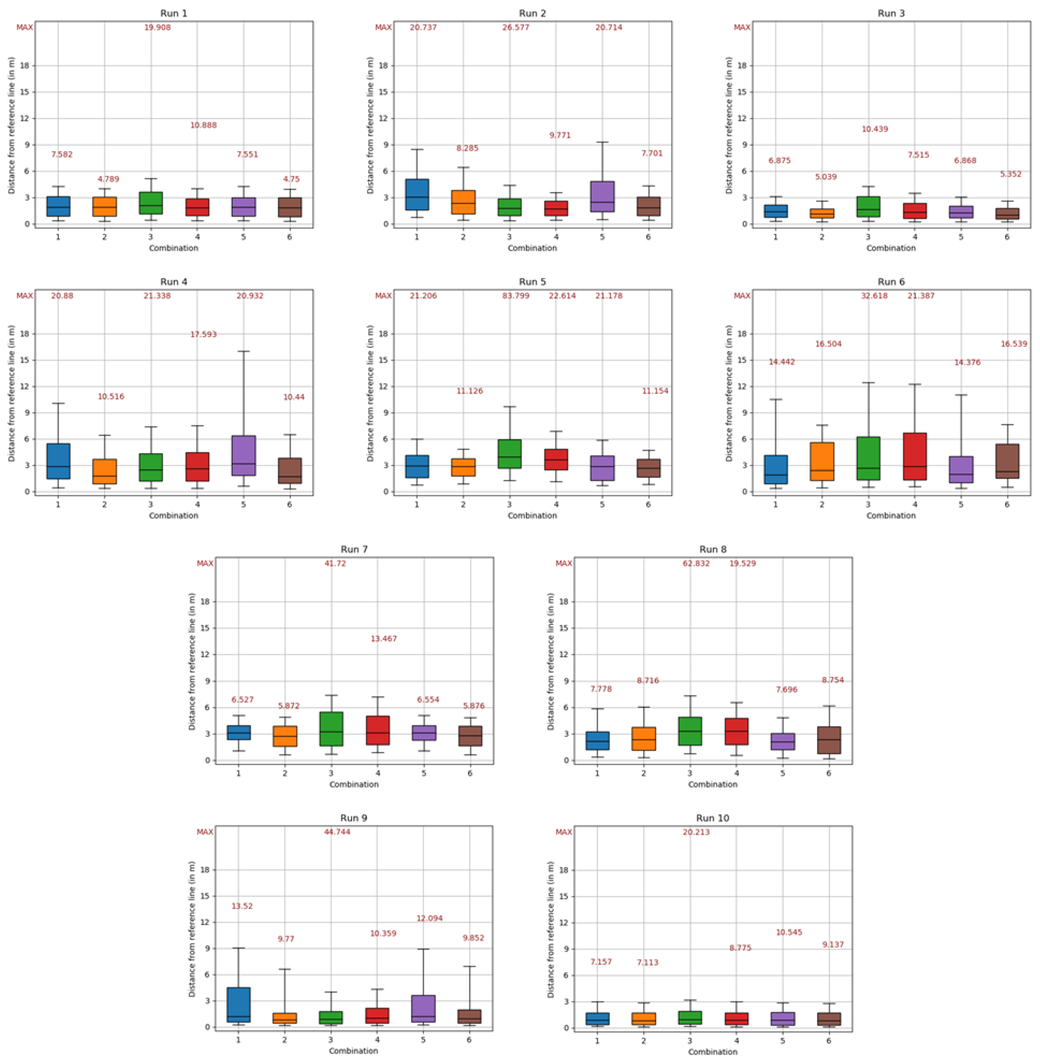
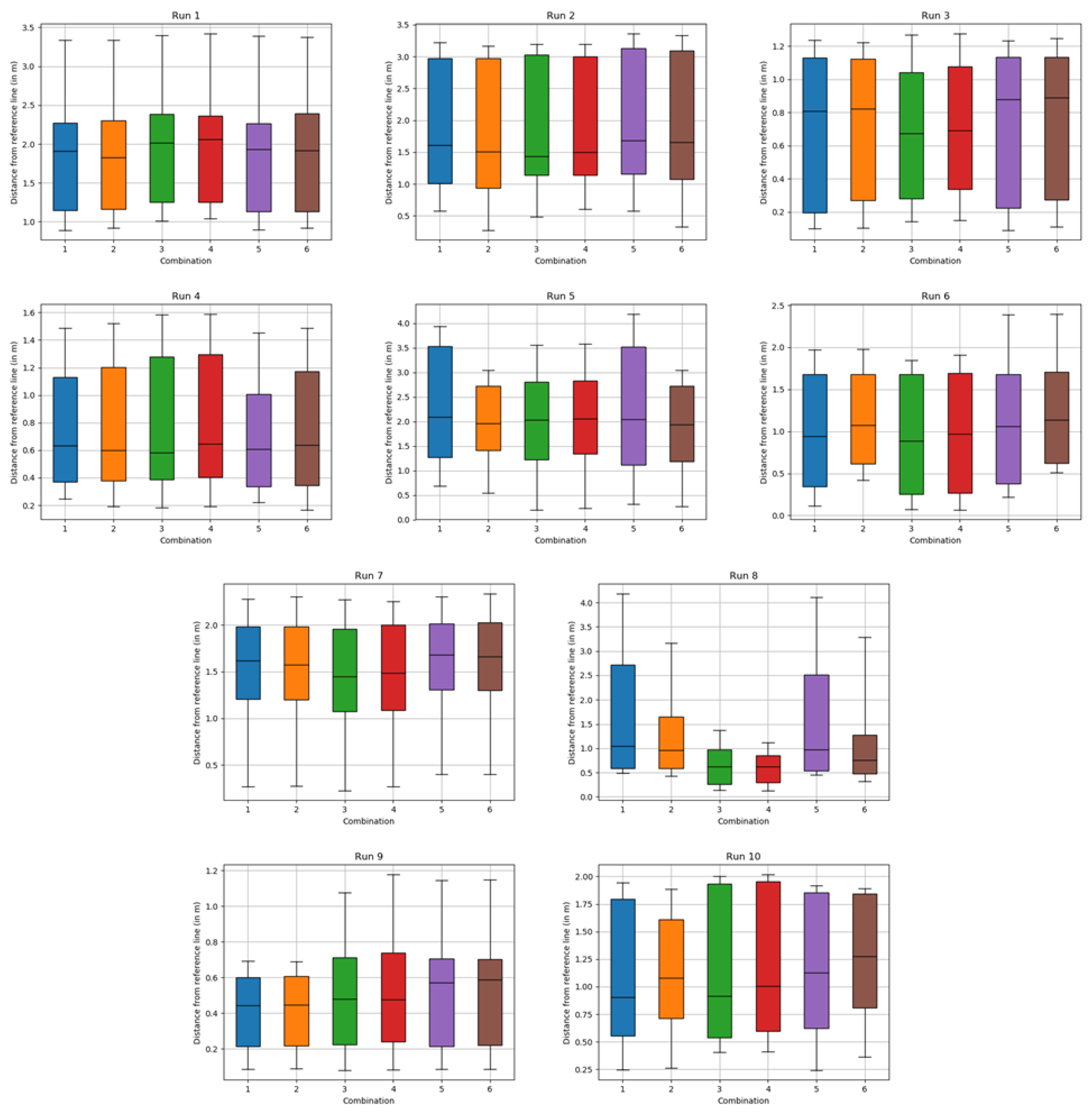
• Distance from the reference tracks: Mean perpendicular distance of the mapped center lines from the reference tracks, measured at every 10 meters.
• Completeness of the result: Percentage of the track that was automatically mapped. Higher percentage implies higher completeness and vice versa.
• Discontinuity of the result: Average number of line segments representing the tracks. Higher number of line segments implies higher discontinuity and vice versa.

3. Results and Discussion

3.1. Performance of Rules

The mean and maximum distance of the GNSS observations for each rule from the reference track for the 10 runs are given in Figure 4. Rule 1 discarded less than 1% of the points. There was no drop in the maximum distance, except in runs 1 and 9, indicating that the points far away from the reference track had more than 4 visible satellites, but still their positional accuracy was poor. On an average, Rule 2 discarded about 1.177% of the points. There was a drop of about 32.486 m (averaged over 10 runs) in the maximum distance, implying that the Rule was successful in discarding points far from the reference line. However, some points that were at a distance of 10 to 15 m from the reference track had passed the rule. One major issue with HDOP is that it does not take into account the local obstructions. Even with a good satellite geometry (that leads to a lower HDOP value), the signals might bounce off the objects around the receiver on its path, thus travelling a longer distance than the straight line distance between the satellite and the receiver. This leads to errors in the computed position. This is called the multi-path effect [11,25,29]. Research has been done to identify these effects using a 3D model of the environment [25,29,30] or using Signal-to-Noise Ratio (SNR) values [31,32,33,34,35]. However, this effect has not been considered in the current work.

On applying Rule 3, the mean and maximum distances were even lower than those of Rule 2 in 7 out of 10 runs, indicating that this Rule was also successful. On an average, the maximum distance reduced by 32.447 m. Rule 3 discarded 68.11% of the points, on an average. The Combined Rule had the lowest mean and maximum distances and could discard most of the points that were more than 10 m away from the reference track. Comparing with the initial dataset, the maximum distance had dropped by 43.020 m after applying the three rules. It was also found that the HDOP (Rule 2) and speed difference (Rule 3) rules complemented each other. Some points far from the reference track passed one of these rules, but failed the other rule. On an average, 67.69% of the points passed the Combined Rule.

3.2. Effect of Conditional Selection of GNSS Data on Kalman Filter Framework

Figure 5 shows the boxplot of perpendicular distance of the mapped main track of combinations 1 (without conditional selection) and 2 (with conditional selection) to the reference track for 10 runs. The whiskers in the boxplots extend from the 10th to the 90th percentile. All distributions are right-skewed. In terms of completeness and discontinuity, both the combinations were able to map almost 100% of the main track as a single line. However, the result from combination 2 was closer to the reference track than the result from combination 1, except in runs 6 and 8, wherein the Conditional Selection of GNSS data had discarded too many points in some sections of the track, causing the result from Kalman filter framework to deviate from the true position. One such example is shown in Figure 6 wherein the Kalman filter could not perform measurement update for about 40 seconds (The RailDriVE was moving at a speed of approximately 27 km/h). Most of the sections of the track far from the reference track were found in areas covered by trees (also see Appendix D.3). The GNSS observations had huge errors in these areas and the Kalman filter framework was able to considerably reduce the uncertainty in position, even with all GNSS observations as input (combination 1). Furthermore, the three rules were successful in removing most of the erroneous observations in these areas, leading to an enhancement of the results from Kalman filter framework. On the other hand, the quality of the GNSS observations in areas with no obstructions were already good before applying the rules. The results from combinations 1 and 2 were very similar (averaged difference in mean and maximum distance was 0.104 m and 0.710 m respectively) in these areas.

If the Conditional Selection of GNSS data takes into account the multi-path effects, it might produce a further improved subset of GNSS observations with which the Kalman filter framework could produce better results. Additionally, a quality score could be calculated for each point to represent how well the point passed each rule. This could be used in the Kalman filter as a measure of the error associated with each GNSS measurement.

3.3. Effect of Weather on Extraction of Center Lines from Laser Scanner Data

In all the combinations with laser scanner data (combinations 3 to 6), 80% to 95% of the main track was automatically mapped, except in runs 9 and 10, where about 30.114% and 75.055% respectively were mapped. It was raining during run 9. During run 10, it was not raining but the ground was still wet. The RSSI value of points that hit the rails was lower when the ground was wet, than it was during sunny conditions because increase in moisture leads to higher specular reflection and lesser scattering [27]. Since a constant set of threshold values were used in the algorithm, which were not suitable for these runs, there were too many false positives and subsequent steps failed to properly map the tracks. This effect is illustrated with an example in Figure 7 which shows a section of the point cloud from run 1 and run 9 ((a) and (b)), the rail points identified at the end of Step 1 of the algorithm ((c) and (d)) and the center lines generated from the point cloud ((e) and (f)). Hence, the result from runs 9 and 10 were skipped for calculating the metrics for evaluating the performance of combinations 3 to 6 (Section 3.4, Section 3.5 and Section 3.6). A different set of threshold values could be used in Step 1 of the center line extraction algorithm in runs 9 and 10 for improved mapping.

3.4. Effect of Conditional Selection of GNSS Data on Extraction of Center Lines from Laser Scanner Data

The automatically identified track center line from combination 3 (mean distance: 2.146 m, maximum distance: 37.404 m; averaged over 8 runs) was farther from the reference tracks than combination 4 (mean distance: 1.806 m, maximum distance: 15.346 m; averaged over 8 runs) because the point cloud from laser scanner was georeferenced using unfiltered set of GNSS points in combination 3. The center lines were far from the reference tracks wherever the error in GNSS observation was large.

Table 3. Averaged Completeness and Discontinuity of tracks mapped in combinations 3 to 6.

Metric		Main Track	First Parallel Tracks	Second Parallel Tracks
Completeness (%)	C3	81.31	57.15	32.30
	C4	85.42	64.23	38.06
	C5	94.85	71.80	39.41
	C6	94.28	69.79	40.40
Discontinuity	C3	1805	9.013	4.508
	C4	795.6	6.199	3.955
	C5	461.5	8.841	3.576
	C6	455.4	3.839	3.525

shows the completeness and discontinuity, averaged over runs 1 to 8, for the main track and first and second parallel tracks. Both the metrics had better values in combination 4 than combination 3, mainly because of the removal of erroneous GNSS observations. Similar to the results in Section 3.2, the results were greatly affected in tree-covered areas (also see Appendix D.3). In areas with no obstructions, the result of combinations 3 and 4 were very close (averaged difference in mean and maximum distance was 0.052 m and 0.291 m respectively). However, one major problem in both the combinations was the noise in the heading values from the GNSS receiver, due to which laser scans were not properly oriented in the point cloud, leading to higher discontinuity values. This issue was fixed by the use of Kalman filters in combinations 5 and 6.

3.5. Effect of Kalman Filter Framework on Extraction of Center Lines from Laser Scanner Data

The Kalman filter framework was very successful in reducing the noise in the heading values (as illustrated in Figure 8), which was the main problem in combinations 3 and 4. Therefore, in combinations 5 and 6, the laser scans were oriented in a much better way while georeferencing the point cloud, which led to improved mapping of center lines. This, in turn, increased the completeness and decreased the discontinuity values. The completeness and discontinuity averaged over runs 1 to 8 for the main and parallel tracks in combinations 5 and 6 are given in Table 3. However, the Conditional Selection of GNSS data did not affect these values, that is, the completeness and discontinuity of results from combinations 5 and 6 were very close in all runs. Furthermore, another source of error in the generation of the point cloud is the vibration of the laser scanner. This could also be a reason for discontinuity in results from processing the point cloud. In order to compensate for this effect, a tilt sensor could be attached close to the laser scanner to measure the vibration experienced by it and these measurements can be used while georeferencing the point cloud.

3.6. Comparison of the Result from the Six Combinations

The boxplot of perpendicular distance of the results from the reference tracks for all combinations for the entire main track, sections of the main track in tree-covered areas, and the sections of the main track in areas without obstructions are given in Appendices Appendix D.1, Appendix D.2 and Appendix D.3 respectively. The mean perpendicular distance from the reference track for combinations 2, 4 and 6 which use the rule-set to select GNSS observations of good quality were 1.48 m, 1.63 m and 1.48 m, respectively. The corresponding maximum distances were 9.41 m, 14.64 m and 9.60 m. The mean perpendicular distance from reference track for combinations 1, 3 and 5 which do not use the rule-set were 1.64 m, 1.91 m and 1.66 mm respectively. The corresponding maximum distances were 13.20 m, 36.42 m and 13.62 m. The distances were lower for all the combinations used the rule-set, when compared with that of the respective combinations not using the rule-set, primarily in areas covered by trees.

A short section of the track in a tree-covered area with the results of all combinations and the reference line is given in Figure 9a. Among the combinations using the rule-set, the result from combinations 2 and 6 were the closest to the reference track (maximum perpendicular distance of 8.77 m and 8.95 m respectively). The result from combination 3 was the farthest from the reference track in all runs (maximum perpendicular distance of 36.42 m), the reason being the use of unfiltered set of GNSS data consisting of erroneous observations and noisy heading values, as pointed out previously in Section 3.4 and Section 3.5. With respect to completeness and discontinuity, combinations 1 and 2 could map almost 100% of the main track as a single line (as explained in Section 3.2), whereas combinations 3 to 6 could map between 80% to 95% of the main track, but as several line segments which will have to be joined manually before using it for other applications (See Table 3).

After looking at the three metrics, it can be concluded that the best results for the main line were obtained in combination 2, in which the rule-set to select GNSS observations and the Kalman filter framework were used. This combination also performed better than the others in tree-covered areas. The laser scanner data did not provide any significant benefit in mapping the main track. Nevertheless, in areas with no obstructions around the railway track, all combinations performed equally good (one example is shown in Figure 9b). So, in these parts, the conditional selection did not provide any significant benefit. It is also important to mention that the Kalman filters used in this work required to make measurement updates without a long gap, without which the results had deviated from the true position (as explained in Section 3.2). Even though they were able to give good results for the sections of tracks in areas covered by trees, they might not work well in tunnels, where there would be no visible satellites for the time period the measurement vehicle moves in the tunnel. Therefore, the Kalman filters need to be adjusted so that it can cope with longer intervals without measurement updates.

The parallel tracks were mapped in combinations 3 to 6. Similar to the main track, combination 3 gave the poorest results, with the lowest completeness and highest discontinuity, as given in Table 3. The results were from either combinations 5 or 6 had the highest completeness and lowest discontinuity, and 60% to 85% of the first parallel tracks and 25% to 65% of the second parallel tracks were automatically mapped. Unlike the previous case with the main track, none of the combinations could map the first and second parallel tracks completely as a single line. Therefore, the line segments have to be manually joined. Nevertheless, the use of RSSI values from the laser scanner reduced false positives in the detection of laser points that had hit rails, providing additional proof to the observation made by Yang and Feng [3] that RSSI values are useful in distinguishing rails from the surrounding entities such as sleepers and ballast. On the other hand, it was also observed that the center line detection algorithm was not very successful in generating center lines at switches. Though the rail points were identified continuously in Step 1, the subsequent steps did not connect them properly as shown in Figure 10. Therefore, the algorithm that connects the points by lines needs to be improved.

The second parallel tracks, which were at a distance of about 10 meters from the main track were less completely mapped when compared with the main track and first parallel tracks with a mean difference in completeness of 51.42% and 27.70% respectively. A similar result was observed in the work by Yang and Fang [3], where the second parallel tracks were not properly detected. However, in the study by Elberink and Khoshelham [4], the detection became noisy from the fourth parallel track. They had used two 360° laser scanners, but the height at which they were mounted on the vehicle is not mentioned. Nevertheless, mounting the laser scanner of the RailDriVE at a higher position could improve the mapping of second parallel tracks (and beyond). Additionally, the algorithm of center line extraction can be improved by applying corrections to the RSSI values from laser scanner. The RSSI values were not taken into account for the detection of the second parallel tracks as the drop in RSSI value was not prominent. These values are affected mainly by the distance between the object and laser scanner, incidence angle, material of the object and atmospheric and instrumental errors. In order to improve the detection of the parallel tracks, existing methods to apply corrections to RSSI values [36,37,38] can be used. In addition to that, the window sizes and threshold values in Step 1 of the center line extraction algorithm could be altered to potentially improve the performance of the method.

In another study using data collected from a terrestrial platform [3], an overall completeness of 95.42% for the detected rails (main track and parallel tracks together) was achieved, which they had calculated by overlaying them on Google Earth imagery. In the current work, 99.91%, 91.48% and 90.81% of the tracks were mapped in combinations 2, 5 and 6 respectively (combination 2 gave the best result for the main track, and combinations 5 and 6 for parallel tracks). Nevertheless, it must be noted that they had collected their measurement data in an environment with few obstructions and had detected rails, not center lines. Other works with related methods, cited in Section 1 were not comparable with the current work for varying reasons. For instance, References [1,10] had used data collected from an aerial platform. Reference [5] had fitted models to the point cloud from laser scanner and evaluated the accuracy of model fitting, whereas the current study evaluated the positioning, completeness and discontinuity of the results. Another reason is the difference in the nature of the reference dataset used. For instance, Reference [4] had used for evaluation the laser scanner data collected by a system different from the system that collected their measurement data, whereas the current work used aerial images for evaluation. Furthermore, the cited works do not provide sufficient details on GNSS/IMU data integration. They specify the device they used, but do not provide algorithmic details to enable comparison with one of our combinations. In contrast, our work discusses these in detail.

4. Conclusions

This work demonstrated the use of data from three sensors (a GNSS receiver, an inertial measurement unit (IMU) and a laser scanner) to automatically map the center line of railway tracks. The aim of this research was to compare six combinations of methods that employ different sensor data: (i) conditional selection of GNSS data, (ii) combination of the GNSS and IMU data in a Kalman filtering framework, and (iii) extraction of center lines from laser scanner data. The study used a large test dataset (approximately 12 Gigabytes) collected using the DLR measurement vehicle RailDriVE which was driven ten times on different sections of the same 33 km long railway track. The data were collected under different weather conditions (sunny, rainy and cloudy). The generated center lines were evaluated using reference data manually digitised from freely available aerial images.

The conditional selection of GNSS points (i) was very successful in discarding erroneous GNSS observations, most of which were found to be in areas covered by trees. After conditional selection, the maximum distance of the points from the reference line reduced by 75%. It was found that the combination of methods (i) and (ii) gave the best result for the track on which the measurement vehicle had moved. In tree-covered areas, this combination performed better when compared with results from other combinations, thus proving that this approach can accurately map tracks in such areas. Almost 100% of the track was automatically mapped as a single line. Therefore, the mapped center line can be used for other applications, such as routing without further improvement. In sections of the track with unobstructed view to satellites, method (ii) and the combination of methods (i) and (ii) provided similar results.

For other parallel tracks in the neighborhood of the track on which the measurement vehicle had moved, the combination of methods (ii) and (iii) and the combination of all three methods gave good results. The use of received signal strength indicator (RSSI) values from the laser scanner in method (iii) improved the algorithm by removing false positives in the detection of laser points that hit the rails. 25% to 80% of the parallel tracks were automatically mapped. The tracks that were closer to the track on which the measurement vehicle had moved were mapped better. However, these combinations mapped each center line as multiple line segments which would have to be joined. On the whole, this research provided automated approaches that are able to reliably map the center line of railway tracks, particularly in tree-covered areas.

References

1. Beger, R.; Gedrange, C.; Hecht, R.; Neubert, M. Data fusion of extremely high resolution aerial imagery and LiDAR data for automated railroad centre line reconstruction. ISPRS J. Photogramm. Remote Sens. 2011, 66, S40–S51. [Google Scholar] [CrossRef]
2. Arastounia, M. An Enhanced Algorithm for Concurrent Recognition of Rail Tracks and Power Cables from Terrestrial and Airborne LiDAR Point Clouds. Infrastructures 2017, 2, 8. [Google Scholar] [CrossRef] [Green Version]
3. Yang, B.; Fang, L. Automated Extraction of 3-D Railway Tracks from Mobile Laser Scanning Point Clouds. IEEE J. Sel. Top. Appl. Earth Obs. Remote Sens. 2014, 7, 4750–4761. [Google Scholar] [CrossRef]
4. Elberink, S.O.; Khoshelham, K. Automatic Extraction of Railroad Centerlines from Mobile Laser Scanning Data. Remote Sens. 2015, 7, 5565–5583. [Google Scholar] [CrossRef] [Green Version]
5. Elberink, S.O.; Khoshelham, K.; Arastounia, M.; Benito, D.D. Rail track detection and modelling in mobile laser scanning data. ISPRS Int. Arch. Photogramm. Remote Sens. Spat. Inf. Sci. 2013, 223–228. [Google Scholar] [CrossRef] [Green Version]
6. Arastounia, M. Automated Recognition of Railroad Infrastructure in Rural Areas from LIDAR Data. Remote Sens. 2015, 7, 14916–14938. [Google Scholar] [CrossRef] [Green Version]
7. Soni, A.; Robson, S.; Gleeson, B. Extracting Rail Track Geometry from Static Terrestrial Laser Scans for Monitoring Purposes. ISPRS Int. Arch. Photogramm. Remote Sens. Spat. Inf. Sci. 2014, 553–557. [Google Scholar] [CrossRef] [Green Version]
8. Hensel, S.; Hasberg, C. Multi Sensor Mapping of Rail Networks. In Proceedings of the 12th International Conference on Information Fusion, Seattle, WA, USA, 6–9 July 2009; pp. 1339–1346. [Google Scholar]
9. Zhu, L.; Hyyppa, J. The Use of Airborne and Mobile Laser Scanning for Modeling Railway Environments in 3D. Remote Sens. 2014, 6, 3075–3100. [Google Scholar] [CrossRef] [Green Version]
10. Neubert, M.; Hecht, R.; Gedrange, C.; Trommler, M.; Herold, H.; Krüger, T.; Brimmer, F. Extraction of Railroad Objects from Very High Resolution Helicopter-borne Lidar and Ortho-image Data. Int. Arch. Photogramm. Remote Sens. Spat. Inf. Sci. 2008, 38, 25–30. [Google Scholar]
11. Teunissen, P.J.; Montenbruck, O. (Eds.) Springer Handbook of Global Navigation Satellite Systems; Springer International Publishing: New York, NY, USA, 2017. [Google Scholar] [CrossRef]
12. Fakharian, A.; Gustafsson, T.; Mehrfam, M. Adaptive Kalman Filtering Based Navigation: An IMU/GPS Integration Approach. In Proceedings of the International Conference on Networking, Sensing and Control, Delft, The Netherlands, 11–13 April 2011; pp. 181–185. [Google Scholar] [CrossRef]
13. Li, Y.; Wang, J.; Rizos, C.; Mumford, P.; Ding, W. Low-cost tightly coupled GPS/INS integration based on a nonlinear Kalman filtering design. In Proceedings of the ION National Technical Meeting 2006, San Diego, CA, USA, 18–20 January 2006; pp. 958–966. [Google Scholar]
14. Zhao, L.; Qiu, H.; Feng, Y. Analysis of a robust Kalman filter in loosely coupled GPS/INS navigation system. Measurement 2016, 80, 138–147. [Google Scholar] [CrossRef]
15. Oh, S.H.; Hwang, D.H. Low-cost and high performance ultra-tightly coupled GPS/INS integrated navigation method. Adv. Space Res. 2017, 60, 2691–2706. [Google Scholar] [CrossRef]
16. Liu, Y.; Fan, X.; Lv, C.; Wu, J.; Li, L.; Ding, D. An innovative information fusion method with adaptive Kalman filter for integrated INS/GPS navigation of autonomous vehicles. Mech. Syst. Signal Process. 2017, 100, 605–616. [Google Scholar] [CrossRef] [Green Version]
17. Falco, G.; Pini, M.; Marucco, G. Loose and Tight GNSS/INS Integrations: Comparison of Performance Assessed in Real Urban Scenarios. Sensors 2017, 17, 255. [Google Scholar] [CrossRef] [PubMed]
18. Roth, M. Advanced Kalman Filtering Approaches to Bayesian State Estimation. Linköping Studies in Science and Technology. Dissertations No. 1832. Ph.D. Thesis, Linköping University, Linköping, Sweden, 2017. [Google Scholar]
19. Gustafsson, F. Statistical Sensor Fusion; Studentlitteratur AB: Lund, Sweden, 2010. [Google Scholar]
20. Särkkä, S. Bayesian Filtering and Smoothing; Cambridge University Press: New York, NY, USA, 2013. [Google Scholar]
21. RailDriVE®. Available online: https://www.dlr.de/ts/desktopdefault.aspx/tabid-10248/17519_read-12871/ (accessed on 27 September 2019).
22. Carstensen, L.W., Jr. GPS and GIS: Enhanced Accuracy in Map Matching through Effective Filtering of Autonomous GPS Points. Cartogr. Geogr. Inf. Syst. 1998, 25, 51–62. [Google Scholar] [CrossRef]
23. Langley, R.B. Dilution of precision. GPS World 1999, 10, 52–59. [Google Scholar]
24. Sairo, H.; Akopian, D.; Takala, J. Weighted dilution of precision as quality measure in satellite positioning. IEE Proc. Radar Sonar Navig. 2003, 150, 430–436. [Google Scholar] [CrossRef]
25. Takeuchi, E.; Yamazaki, M.; Ohno, K.; Tadokoro, S. GPS Measurement Model with Satellite Visibility using 3D Map for Particle Filter. In Proceedings of the 2011 IEEE International Conference on Robotics and Biomimetics, Karon Beach, Phuket, 7–11 December 2011; pp. 590–595. [Google Scholar] [CrossRef]
26. Petovello, M. How Does a GNSS Receiver Estimate Velocity? Inside GNSS 2015, 38–41. Available online: https://insidegnss.com/wp-content/uploads/2018/01/marapr15-SOLUTIONS.pdf (accessed on 27 January 2020).
27. Shan, J.; Toth, C.K. (Eds.) Topographic Laser Ranging and Scanning: Principles and Processing; CRC Press: Boca Raton, FL, USA, 2008. [Google Scholar]
28. Geoportal Sachsen. Available online: https://geoportal.sachsen.de/cps/metadaten_portal.html?id=cd01c334-7e32-482f-bd43-af286707178a (accessed on 27 September 2020).
29. Maier, D.; Kleiner, A. Improved GPS Sensor Model for Mobile Robots in Urban Terrain. In Proceedings of the 2010 IEEE International Conference on Robotics and Automation, Anchorage, AK, USA, 3–7 May 2010; pp. 4385–4390. [Google Scholar] [CrossRef] [Green Version]
30. Wang, L.; Groves, P.D.; Ziebart, M.K. Multi-Constellation GNSS Performance Evaluation for Urban Canyons Using Large Virtual Reality City Models. J. Navig. 2012, 65, 459–476. [Google Scholar] [CrossRef] [Green Version]
31. Bilich, A.; Larson, K.M. Mapping the GPS multipath environment using the signal-to-noise ratio (SNR). Radio Sci. 2007, 42. [Google Scholar] [CrossRef]
32. Bilich, A.; Larson, K.M.; Axelrad, P. Modeling GPS phase multipath with SNR: Case study from the Salar de Uyuni, Bolivia. J. Geophys. Res. Space Phys. 2008, 113. [Google Scholar] [CrossRef]
33. Lau, L.; Cross, P. A New Signal-to-Noise-Ratio Based Stochastic Model for GNSS High-Precision Carrier Phase Data Processing Algorithms in the Presence of Multipath Errors. In Proceedings of the 19th International Technical Meeting of the Satellite Division of The Institute of Navigation (ION GNSS 2006), Fort Worth, TX, USA, 26–29 September 2006; pp. 76–285. [Google Scholar]
34. Strode, P.R.R.; Groves, P.D. GNSS multipath detection using three-frequency signal-to-noise measurements. GPS Solut. 2016, 20, 399–412. [Google Scholar] [CrossRef] [Green Version]
35. Benton, C.J.; Mitchell, C.N. Isolating the multipath component in GNSS signal-to-noise data and locating reflecting objects. Radio Sci. 2011, 46. [Google Scholar] [CrossRef] [Green Version]
36. Kaasalainen, S.; Jaakkola, A.; Kaasalainen, M.; Krooks, A.; Kukko, A. Analysis of Incidence Angle and Distance Effects on Terrestrial Laser Scanner Intensity: Search for Correction Methods. Remote Sens. 2011, 3, 2207–2221. [Google Scholar] [CrossRef] [Green Version]
37. Krooks, A.; Kaasalainen, S.; Hakala, T.; Nevalainen, O. Correction of Intensity Incidence Angle Effect in Terrestrial Laser Scanning. ISPRS Ann. Photogramm. Remote Sens. Spat. Inf. Sci. 2013, 2, 145–150. [Google Scholar] [CrossRef] [Green Version]
38. Höfle, B.; Pfeifer, N. Correction of laser scanning intensity data: Data and model-driven approaches. ISPRS J. Photogramm. Remote Sens. 2007, 62, 415–433. [Google Scholar] [CrossRef]
Figure 1. Workflow for the investigated combinations of methods. The figure illustrates how the global navigation satellite system (GNSS), inertial measurement unit (IMU), and laser data are processed using combinations (indicated by arrows of different colors) of three different methods (blue boxes) to yield center lines of railway tracks.
Remotesensing 12 00411 g001
Figure 2. Terms used in the description of the algorithm. Image source: Camera mounted on RailDriVE.
Remotesensing 12 00411 g002
Figure 3. Plot of Height (in mm) and RSSI values of points in one sweep made by the laser scanner.
Remotesensing 12 00411 g003
Figure 4. (a) Mean and (b) Maximum distance of the GNSS points from the reference track while applying the rules.
Remotesensing 12 00411 g004
Figure 5. Boxplots of perpendicular distance of the mapped track from combinations 1 (blue) and 2 (orange) to the reference track. The numbers in red are the maximum distances from the reference line.
Remotesensing 12 00411 g005
Figure 6. A section of the track where the result from Kalman filter had deviated due to fewer measurement updates.
Remotesensing 12 00411 g006
Figure 7. Illustration of the effect of weather on center line mapping process. (a,b): Georeferenced point cloud. (c,d): Points identified as rails in Step 1 of the algorithm. (e,f): Centerlines extracted from the point cloud.
Remotesensing 12 00411 g007
Figure 8. Heading values of a portion of the data in combinations with (5 and 6) and without (3 and 4) Kalman filter framework.
Remotesensing 12 00411 g008
Figure 9. Map of result of all combinations and the reference line in (a) tree-covered area (result from combinations 1 and 5 as well as 2 and 6 are similar in this section of the track) and, (b) area with no obstructions (result from all combinations are similar in this section of the track).
Remotesensing 12 00411 g009
Figure 10. Rail points and center lines identified in two different sections (a,b) of the track with a switch.
Remotesensing 12 00411 g010