Assessment of UAV-Onboard Multispectral Sensor for Non-Destructive Site-Specific Rapeseed Crop Phenotype Variable at Different Phenological Stages and Resolutions

Abstract

Unmanned aerial vehicles (UAVs) equipped with spectral sensors have become useful in the fast and non-destructive assessment of crop growth, endurance and resource dynamics. This study is intended to inspect the capabilities of UAV-onboard multispectral sensors for non-destructive phenotype variables, including leaf area index (LAI), leaf mass per area (LMA) and specific leaf area (SLA) of rapeseed oil at different growth stages. In addition, the raw image data with high ground resolution (20 cm) were resampled to 30, 50 and 100 cm to determine the influence of resolution on the estimation of phenotype variables by using vegetation indices (VIs). Quadratic polynomial regression was applied to the quantitative analysis at different resolutions and growth stages. The coefficient of determination (R²) and root mean square error results indicated the significant accuracy of the LAI estimation, wherein the highest R² values were attained by RVI = 0.93 and MTVI2 = 0.89 at the elongation stage. The noise equivalent of sensitivity and uncertainty analyses at the different growth stages accounted for the sensitivity of VIs, which revealed the optimal VIs of RVI, MTVI2 and MSAVI in the LAI estimation. LMA and SLA, which showed significant accuracies at (R² = 0.85, 0.81) and (R² = 0.85, 0.71), were estimated on the basis of the predicted leaf dry weight and LAI at the elongation and flowering stages, respectively. No significant variations were observed in the measured regression coefficients using different resolution images. Results demonstrated the significant potential of UAV-onboard multispectral sensor and empirical method for the non-destructive retrieval of crop canopy variables.

1. Introduction

Applications of the unmanned aerial vehicle (UAV) platform in precision agriculture (PA) offered a precise and reliable solution for the optimisation of crop monitoring and management [1]. UAV in PA is a new but reliable remote sensing tool that can acquire high spectral, spatial and temporal resolution data and has the advantages of low cost, flexible platform and bird’s eye view for rapid data collection [2,3]. UAV in PA can customise the imaging sensor to meet the spectral and spatial requirements and to achieve fast utilisation [4]. Compared with other remote sensing platforms, UAVs can fly at low altitudes and can capture high-resolution imagery, which offers very detailed spectral and spatial descriptions of the field [1,4]. For highly dynamic vegetation monitoring, the UAV-onboard sensor allows the precise determination of plant location during the growing season to act with corrective measures [2,4,5]. The timely monitoring of crop dynamics is critical in addressing various forms of environmental issues, agricultural practices, degasses and pest control that can eventually lead to enhanced production [6,7,8]. UAV, sensors and other geospatial techniques (e.g., GIS, remote sensing and GPS) help in determining field variations and optimum fertilisation, disease diagnosis and pest control for sustainable production; this type of determination process is called PA [2,9]. The application of remote sensing in agriculture has become an important research direction because it provides valuable information in terms of agronomic parameters, which facilitate sustainable crop monitoring. Remote sensing data also produce repeated and useful non-destructive crop biophysical attributes for PA [7,10]. Gathering these information required for the enhancement of agricultural production in PA is the key issue that requires the use of a proper design and decision-making system [2,11].

The data collected through the aerial and satellite approaches of remote sensing are useful; however, these platforms are limited by temporal and spatial resolutions, cloud covers and operational costs [12,13]. During the last decade, UAV has been typically used in crop monitoring with high-spatial resolution imagery, low operational cost and near-real-time data acquisition based on powerful sensor-bearing ideal platforms for mapping and monitoring [2,14,15]. In the practical applications of remote sensing techniques in PA, various agricultural equipment units have been developed but require major improvements to meet the variation requirements of seasonal patterns in numerous indices that are used in agronomic evaluations [7].

Leaf area index (LAI), leaf mass per area (LMA) and specific leaf area (SLA) are leaf functional traits that provide information about vegetation canopies in the functional diversity assessment and quantification of physiological processes to prescribe optimum management strategies [16]. These traits correspond to the analytical variables of the plant physiological process, such as growth rates, photosynthetic capacity and plant life strategies [17]. LAI refers to the one-sided green leaf area per unit of ground surface area and is a dimensionless parameter that characterises photosynthesis and respiration and defines the functional link to the canopy spectral reflectance [8,10,18]. LMA is calculated as the ratio of leaf dry mass to leaf area, which is a key biophysical variable involved in plant light capture and carbon gain [19]. Numerous studies identified its significance to the photosynthesis–nitrogen relationship and other essential characteristics, such as the leaf mass-based nitrogen content, which can be inferred from the remote sensing data as the leaf dry mass composed of several organic elements that absorb radiation at a fixed wavelength [19,20]. SLA refers to the leaf area per unit of dry leaf mass or the leaf mass per unit area, which are usually expressed in m²/kg. SLA is an important trait associated to the plant growth rate, which provides information about photosynthetic capacity and leaf nitrogen variations [17]. This trait is indicative of the physiological processes, such as growth rate, light capture and survival [21].

Crop growth and yield models require the estimates of crop biophysical parameters and the association of infrared reflectance to the biophysical parameter of crop canopies that offer the tool for linking multispectral remote sensing to crop growth behaviour [8]. For instance, the soil and water assessment tool model uses the maximum LAI as the key parameter that influence crop growth and watershed flow routing; this parameter can also be changed according to the agronomists’ feedback [22,23]. Agricultural studies need to compute and monitor the biochemical and biophysical properties of plants for crop growth, chlorophyll content, nitrogen content and LAI that provide clues to crop health and productivity. Compared with direct field surveys, the remote sensing techniques for the acquisition of these parameters are performed in real time, are non-destructive and provide the spatial details for the measurement and monitoring of these parameters. The empirical relationship between the biophysical parameters and spectral vegetation indices (VIs) has been developed and used to address the relationship between crop traits and canopy reflectance. The empirical relationship of spectral data is effective in predicting the crop biophysical traits because of its simplicity and ability to capture various canopy variations, and this approach is widely used because of its ease in computation [24].

VIs have been developed as a mathematical combination of various spectral bands of the electromagnetic spectrum and are related to various canopy parameters, which can enhance the vegetation signals by reducing the atmospheric and soil effects. The spectral VIs measure vegetation activity and demonstrate the spatial variations of the different seasons through space [7,25]. Substantial developments have been made in the interpretation and analysis of the spectral VIs, which have been applied from the field to the global level [25]. However, these indices are species-specific and are therefore not robust in different species with various leaf and canopy architectures [2,7,25].

Several studies regarding the application of UAV in rice crop yield and biomass estimation have been published [13]. The UAV application in sunflower crop has shown a significant correlation between normalized difference vegetation index (NDVI) and grain yield biomass and applied nitrogen content [2], whereas the UAV platform (‘VIPtero’) for onboard multispectral camera in vineyard management demonstrated a clear crop heterogeneity, which was consistent with the ground observations [9]. The multispectral sensor mounted on a UAV over potato crops demonstrated a significant correlation between NDVI and green normalized vegetation index (GNDVI) with LAI, plant cover and chlorophyll content [12].

Although the application of UAV has progressed considerably, it still has many limitations, such as payload, cost and operation consistency in agriculture. Thus, a substantial amount of work is still required. UAVs capture numerous high-resolution images that require lengthy processing times, high storage devices and high labour intensity even for professionals because of its low-altitude image acquisition capability [26,27]. Fine-resolution VIs demonstrated a significant influence on the accuracy of prediction models [28]. Although studies have determined that high-resolution images might not be the optimal choice for environmental variable and concluded that fine-resolution VIs obtain a similar prediction model accuracy [2,29,30]. The measuring scale is dependent on the association between biophysical traits and VIs from images with different resolutions, which can help select the appropriate resolution for site-specific management.

Remotely sensed VIs can offer significant information derivatives to agronomic parameters at the field scale. Therefore, the sensor that can monitor crops during the growth season at high spectral, spatial and temporal resolutions will provide useful information in the efficient and sustainable crop management with site-specific basis. Amongst the phenotypical parameters derived using remotely sensed data, LMA and SLA have received minimal attention. However, the retrieval of the mentioned parameters using the radiative transfer model (RTM) inversion could be ill-advised and computationally demanding because it requires a number of leaf and canopy variables. In this study, we optimised and validated numerous VIs for LAI and leaf dry weight (DW) prediction and investigated the potential of empirically estimated LAI and DW for the estimation of the two leaf functional traits, namely, LMA and SLA. Therefore, our study mainly aims to (1) evaluate the potential of a multispectral sensor onboard a UAV in relation to crop biophysical parameters, such as LAI and DW, during the growing season over rapeseed crops at different phenological stages, (2) assess the spectrally predicted leaf DW and LAI for the calculation of LMA and SLA at different phenological stages and (3) assess the effects of resolution on the LAI prediction over the phenological stages to provide simple, rapid and useful information for PA.

2. Materials and Methods

2.1. Study Area

The field experiment was conducted at the Zishi experimental station of Huazhong Agricultural University in Jingzhou (30°11′28.62″ N, 112°23′31.61″ E) located in the south-central part of Hubei Province, China from 18 December 2017 to 10 March 2018. This area has a subtropical monsoon climate with an average rainfall of 1100–1300 mm, average annual temperature of 15.9 °C to 16.6 °C, hydrothermal synchronisation and consistent good climatic condition suitable for agricultural activities. Winter rapeseed was used as the experimental material in this study. To imitate the high variability of growing conditions and investigate the spectral VIs for the estimation of crop phenotype parameters, the data were collected from 16 different fields and 170 point locations. The experimental fields and sampling points are presented in Figure 1.

2.2. Biophysical Parameter Measurements

The non-destructive LAI was measured using a plant canopy analyser (SunScan, Probe type SS1, Delta-T Devices, England) over all point locations (Figure 1) after 55 days of plantation on 18 December 2017, after 79 day of plantation on 11 January 2018, 106 days after plantation on 7 February 2018 and after 138 day of plantation on 10 March 2018 according to the crop growth stages from seedling to maturity during the growing season. Measurements were obtained on clear cloudless days. At each phenological stage, 30 subsampling points were selected randomly, and four plants were sampled destructively with their roots. The plant density was also recorded in each point, location, latitude and longitude. The samples were stored in bags and moved to the laboratory. The leaves, stems and roots of the samples were separated to obtain their fresh weights and then placed in an oven at 70 °C for 48 hours to obtain the dry mass. The fresh and dry weights of each leaf sample were determined using a high-precision digital scale. LMA and SLA were calculated as follows:

$$LMA=Dw/LA$$

(1)

where Dw and LA are the leaf DW and leaf area, respectively.

$$SLA=LA/Dw$$

(2)

where LA and Dw are the leaf area and the corresponding Dw, respectively [17,31].

2.3. UAV Image Acquisition

Multispectral images were also acquired on the days of LAI measurement using the UAV platform. Prior to the flight campaign, the camera was mounted on the UAV under suitable working condition. A lightweight RedEdge MicaSense multispectral camera (MicaSense RedEdge®) onboard a fixed-wing UAV (T-EZ; Golden Wing UAS Co., Ltd.; Chengdu, China) was used to capture the field images shown in Figure S1. A stable platform was used to adjust the camera pointing towards the nadir. The spectral bands covered the wavelength intervals 450 nm centre, 20 nm bandwidth (blue), 560 nm centre, 20 nm bandwidth (green), 668 nm centre, 10 nm bandwidth (red), 717 nm centre, 10 nm bandwidth (RedEdge), 840 nm centre and 40 nm bandwidth (near-infrared). After take-off, the UAV was programmed to follow the predefined route and complete the flight campaign. The flight altitude was 300 m and resulted in a ground resolution of 20 cm.

2.4. Image Processing

The raw multispectral images acquired by the RedEdge camera were processed in terms of image mosaicking, vignetting correction and raw digital number (DNs) for the reflectance conversion using the Pix4Dmapper (Pix4D SA, Switzerland) software. The raw digital numbers of the acquired images were firstly converted into radiance and then into surface reflectance based on the linear regression models by using the calibration target data, wherein the surface reflectance is a linear function of the digital numbers [32]. In each stage, 1024 images were captured and mosaicked from the study area, and the georeferenced images of the study area were acquired at the end of the fourth crop season. Moreover, the raw images with the ground resolution of 20 cm were resampled to 30, 50 and 100 cm by using the pixel aggregate interpolation method to assess the influence of image resolution on VIs. Lastly, the VIs were calculated.

2.5. Multispectral VIs

The canopy spectral data were used to develop the VIs, which are sensitive to canopy structure, pigments and chlorophyll, for the LAI, LMA and SLA estimation in rapeseed crops. Nine VIs were calculated, several of which have been proposed as surrogates for LAI estimation [10,25,32]. The calculated VIs, their formula and description are listed in

Table 1. Description and formulas of the investigated VIs.

Indices	Formulas	Description	References
RVI	$RVI={\rho }_{nir}/{\rho }_{red}$	Sensitive to nitrogen	[33,10]
NDVI	$NDVI=\left({\rho }_{nir}-{\rho }_{red}\right)/\left({\rho }_{nir}+{\rho }_{red}\right)$	Structure (LAI, fraction) Chlorophyll content	[34]
GNDVI	$GNDVI= \left({\rho }_{nir}-{\rho }_{green}\right)/\left({\rho }_{nir}+{\rho }_{green}\right)$	Biomass, LAI, photosynthesis and plant stress	[7,35]
BNDVI	$BNDVI=\left({\rho }_{nir}-{\rho }_{blue}\right)/\left({\rho }_{nir}+{\rho }_{blue}\right)$	Chlorophyll content	[36]
SAVI	$SAVI=\frac{ \left( {\rho }_{nir}- {\rho }_{red}\right)}{ \left({\rho }_{nir}+ {\rho }_{red}+0.5\right)}\left(1+0.5\right)$	Structure (LAI, fraction)	[37,38]
OSAVI	$OSAVI=\left(1+0.16\right)\frac{\left( {\rho }_{nir}- {\rho }_{red}\right)}{\left({\rho }_{nir}+ {\rho }_{red}+0.16\right)}$	Structure (LAI, fraction)	[39,40]
MSAVI	$\mathrm{MSAVI}={\rho }_{nir}+0.5-(0.5\sqrt[ ]{\left(2*{\rho }_{nir}+1\right){ }^2-8({\rho }_{nir}-\left(2*{\rho }_{red}))\right)}$	Structure (LAI, sensitive to canopy effects)	[41]
MSAVI2	$MSAVI2=\frac{1}{2}\left[2{\rho }_{nir}+1-\sqrt{{\left(2{\rho }_{nir}+1\right)}^2-8({\rho }_{nir}-{\rho }_{red}}\right]$	Structure (LAI, fraction)	[41]
MTVI2	$MTVI2=\frac{1.5\left[1.2\left({\rho }_{nir}-{\rho }_{green}\right)-\left(2.5{\rho }_{red}-{\rho }_{green}\right)\right]}{\sqrt{{\left(2{\rho }_{nir}+1\right)}^2-(6{\rho }_{nir}-5\sqrt{{\rho }_{red})}-0.5}}$	Structure (Sensitive to LAI, resistant to chlorophyll influence)	[38]

Note: RVI, ratio vegetation index; NDVI, normalized difference vegetation index; GNDVI, green normalized vegetation index; BNDVI, blue normalized difference vegetation index; SAVI, soil-adjusted vegetation index; OSAVI, optimised soil-adjusted vegetation index; MSAVI, modified soil-adjusted vegetation index; MSAVI2, modified soil-adjusted vegetation index 2; MTVI2, modified triangular vegetation index 2.

. For all VIs, the images with the same resolution were stacked, and the mean VI values centred on the 1 m² location were extracted for 160 point locations in ENVI 5.1 (Exelis Visual Information Solution, Inc.; Boulder, CO, USA).

2.6. Statistical Analysis

Regression models were used for the quantitative analysis between spectral VIs as independent and LAI and leaf DW as dependent variables at the different phenological stages. A total of 140 and 30 sample points for LAI and LD were used for model calibration, respectively, whereas 30 sample points each were used for validation. To assess the model performance, the coefficient of determination (R²), root mean square error (RMSE) and relative RMSE (RRMSE) were used and calculated using Equations. (3), (4) and (5), respectively [18,42,43]. The large R² value and low RMSE and RRMSE values indicated the high precision and accuracy of the model as follows:

$$R^2=1-\frac{{\sum }_{i=1}^n{(y_{i }- {\hat{y}}_i)}^2}{{\sum }_{i=1}^n{(y_i-\overline{y} )}^2}$$

(3)

$$RMSE=\sqrt{\frac{{\sum }_{i=1}^n{(y_i-{\hat{y}}_i)}^2}{n}}$$

(4)

$$RRMSE=\frac{RMSE}{\overline{y}}\times 100$$

(5)

where R² and RMSE measure the relationship of the fitting function. However, for the nonlinear functions amongst LAI and VIs, the R² values may be misleading because sensitivity changes continuously [10]. Thus, a different accuracy matric noise equivalent (NE) was needed to evaluate and determine the LAI estimation accuracy. NE also accounts for the slope and scattering of data points in the best-fit function as follows [10,25,44]:

$$NE\mathsf{\Delta }LAI=\frac{RMSE\left\{VI VS. LAI\right\}}{d\left(VI\right)/d\left(LAI\right)}$$

(6)

where RMSE is the root mean square error of the best-fit function between the spectral Vis and LAI, and $\mathrm{d}\left(\mathrm{VI}\right)/\mathrm{d}\left(\mathrm{LAI}\right)$ is the first-order derivative of the observed relationship.

3. Results

3.1. Association of VIs to the Phenolgical Stages

A wide range of variations in LAI, DW, LMA and SLA due to different canopy architectures as well as variations due to leaf sizes and shapes at different phenological stages was recorded.

Table 2. Descriptive statistics of canopy LAI, DW, LMA and SLA of rapeseed oil at the different phenological stages in the Zishi experimental station.

Phonological stage	Statistics	LAI (m2m−2)	DW (g·cm−2)	LMA (g·cm−2)	SLA (cm2g−1)
Seedling stage	Minimum value	0.2	0.005	0.004	0.001
	Maximum value	4.9	0.051	0.037	0.055
	Mean value	1.72	0.025	0.016	0.012
	Standard deviation	1.13	0.014	0.009	0.012
Elongation stage	Minimum value	0.2	0.008	0.003	0.001
	Maximum value	5.03	0.083	0.087	0.024
	Mean value	2.23	0.038	0.023	0.005
	Standard deviation	1.15	0.019	0.014	0.004
Flowering stage	Minimum value	0.1	0.010	0.002	0.001
	Maximum value	4.83	0.044	0.082	0.032
	Mean value	1.60	0.027	0.023	0.006
	Standard deviation	0.99	0.010	0.014	0.006
Maturity stage	Minimum value	0.1	0.001	0.002	0.001
	Maximum value	3.72	0.052	0.046	0.045
	Mean value	1.74	0.022	0.013	0.007
	Standard deviation	0.70	0.010	0.009	0.008

presents the descriptive statistics of canopy LAI, DW, LMA and SLA of rapeseed oil at the phenological stages in the Zishi experimental station.

All the VIs investigated at the different growth stages revealed close associations with the crop reflectance characteristics. The spectral VIs demonstrated significant variations in all the phenological stages from seedling to maturity, and the results are compiled in

Table 3. Relationship of spectral VIs at the different phenological stages.

	Phenological stages
	R2				RMSE
VIs	Seedling	Elongation	Flowering	Maturity	Seedling	Elongation	Flowering	Maturity
RVI	0.86	0.93	0.89	0.45	0.44	0.30	0.32	0.49
NDVI	0.86	0.88	0.87	0.41	0.47	0.40	0.35	0.54
GNDVI	0.82	0.87	0.82	0.41	0.50	0.41	0.42	0.51
BNDVI	0.82	0.86	0.79	0.44	0.50	0.42	0.44	0.50
SAVI	0.86	0.85	0.83	0.45	0.43	0.44	0.41	0.49
OSAVI	0.85	0.86	0.84	0.49	0.45	0.42	0.40	0.48
MSAVI	0.85	0.87	0.86	0.47	0.44	0.40	0.37	0.49
MSAVI2	0.86	0.85	0.82	0.48	0.43	0.44	0.42	0.48
MTVI2	0.88	0.89	0.86	0.52	0.40	0.38	0.36	0.46

. The VIs attained its peak values at the elongation stage and started to decline afterwards. All the VIs demonstrated a significant relation with LAI at the seedling stage. Furthermore, the MSAVI2, MTVI2 and SAVI showed the most sensitive VIs with an R² value of 0.87, followed by MSAVI (R² = 0.86), whilst NDVI and OSAVI achieved R² = 0.85, GNDVI R² = 0.82 and BNDVI obtained an R² value of 0.81 at the seedling stage. RVI, NDVI, MSAVI and MTVI2 showed the most influenced VIs to LAI from the seedling to maturity stages and attained the maximum R² (0.93–0.89, 0.88–0.86, 0.87–0.86 and 0.89–0.86) from the elongation to flowering stages. The minimum R² values at the maturity stage were expected due to crop senescence.

3.2. Evaluation of Spectral VIs for Estimation of Rapeseed LAI

The optimal spectral VIs for the estimation of the LAI best-fit model relationship for VIs and LAI at all the phenological stages are shown in

Table 4. Quadratic polynomial regression and summary statistics of relationship between LAI and studied VIs based on calibration data set at different phenological stages.

Phenological Stage	VIs	Model	R2	RRMSE
Seedling Stage	RVI	y = 0.0462x2 − 0.1042x + 0.3819	0.86	24%
	NDVI	y = 43.705x2 − 47.037x + 13.056	0.84	26%
	GNDVI	y = 65.417x2 −54.631x + 11.848	0.82	28%
	BNDVI	y = 104.91x2 − 130.44x + 40.965	0.82	28%
	SAVI	y = 46.485x2 − 30.462x + 5.4871	0.86	24%
	OSAVI	y = 44.048x2 − 38.005x + 8.6542	0.85	25%
	MSAVI	y = 24.965x2 − 6.9701x + 0.9874	0.86	25%
	MSAVI2	y = 28.964x2 − 16.621x + 2.9121	0.86	24%
	MTVI2	y = 22.307x2 − 4.5415x + 0.7493	0.88	22%
Elongation Stage	RVI	y = 0.011x2 + 0.5195x − 1.6884	0.93	13%
	NDVI	y = 68.09x2 − 79.03x + 23.531	0.88	17%
	GNDVI	y = 60.213x2 − 48.337x + 10.064	0.87	18%
	BNDVI	y = 119.49x2 − 142.14x + 42.779	0.86	18%
	SAVI	y = 31.046x2 −17.785x + 2.8609	0.85	19%
	OSAVI	y = 43.247x2 − 37.807x + 8.7777	0.86	18%
	MSAVI	y = 18.643x2 − 3.1952x + 0.433	0.88	17%
	MSAVI2	y = 19.239x2 − 8.6972x + 1.2314	0.85	19%
	MTVI2	y = 17.139x2 −1.3713x + 0.3066	0.89	16%
Flowering Stage	RVI	y = 0.1402x2 − 0.273x − 0.2612	0.89	19%
	NDVI	y = 49.059x2 − 46.541x + 11.289	0.87	21%
	GNDVI	y = 42.303x2 − 27.235x + 4.1857	0.82	25%
	BNDVI	y = 94.642x2 − 102.03x + 27.677	0.79	27%
	SAVI	y = 27.79x2 − 17.512x + 2.8845	0.83	25%
	OSAVI	y = 38.042x2 − 31.109x + 6.6067	0.84	24%
	MSAVI	y = 12.155x2 + 1.2127x − 0.3412	0.86	22%
	MSAVI2	y = 26.44x2 − 17.359x + 3.1088	0.82	25%
	MTVI2	y = 15.947x2 − 0.3135x + 0.0678	0.86	22%

. The spectral pattern variations and close association with crop reflectance revealed the potential capability of the explored VIs in LAI estimation. All the VIs demonstrated a high significant relationship to the temporal distribution of LAI at the different growth stages, except at the maturity stage, which revealed the lowest coefficient of determination (R² < 0.50) and were omitted from the calculations. Amongst the investigated phenological stages, all the VIs attained their highest coefficient of determination at the elongation stage, whereas the highest R² value was achieved by RVI (R² = 0.93), followed by MTVI2 (R² = 0.89) at the different phenological stages, as provided in Table 3. At the next flowering phenological stage, R² started to decrease until maturity, and the best-fit model of LAI with spectral VIs provided RVI (R² = 0.89), followed by NDVI (R² = 0.87) and MTVI2, MSAVI (R² = 0.86) and OSAVI (R² = 0.84), whereas SAVI attained R² = 0.83 and GNDVI and MSAVI2 attained R² = 0.82. The least R² value was attained by BNDVI (R² = 0.79). MSAVI and MTVI2 have the modifying factor to deal with the saturation problem when the LAI surpasses the saturation level (LAI > 3), whilst the sensitivity of NDVI suffered and levelled out.

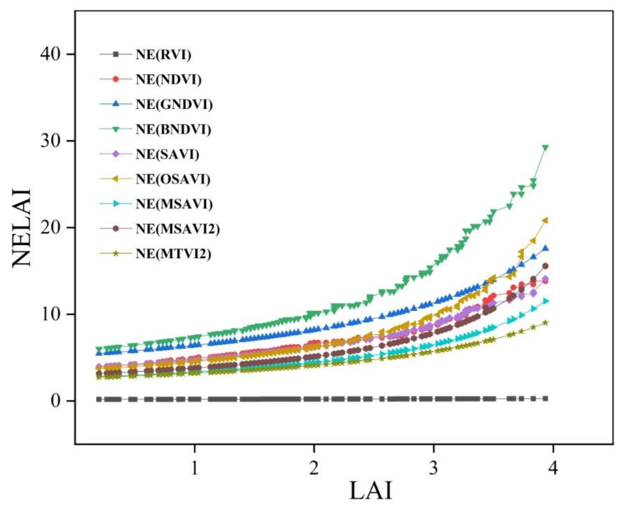
3.3. Sensitivity Analysis

The sensitivity analysis results demonstrated that BNDVI and GNDVI presented the maximum insensitivity, whereas OSAVI exhibited moderately higher sensitivity and was unreliable during the entire range of LAI. NDVI and SAVI exhibited higher sensitivity for LAI < 2.5 m²m⁻² and a decreasing sensitivity trend was observed for higher LAI > 3.0 m²m⁻², whereas MSAVI2 performed better than NDVI and SAVI even at LAI > 3.0 m²m⁻² [25,45]. RVI showed higher sensitivity to LAI and is the best index for the detection of numerical variations in LAI because other indices are not robust at higher LAI values. MSAVI and MTVI2 exhibited higher and consistent sensitivity for LAI < 3.0 m²m⁻², and a decreasing trend was observed for higher LAI > 3.0 m²m⁻² for MSAVI. Therefore, RVI and MTVI2 demonstrated the lowest NE values to ensure the highest sensitivities to LAI and the best multispectral indices for quantitatively detecting variations in LAI (Figure 2).

3.4. Relationship of VIs and Leaf DW

To evaluate the optimal VIs in the estimation of leaf DW (gm⁻²), the best-fit model relationship was used between the leaf DW and VIs presented in Table 1 at the different phenological stages demonstrated in

Table 5. Power function models and summary statistics of the relationship between LD and the explored VIs based on the calibration data set at different phenological stages.

Phenological Stage	VIs	Model	R2	RRMSE
Seedling Stage	RVI	y = 23.32562x1.31245	0.59	38%
	NDVI	y = 1047.82027x3.91124	0.60	38%
	GNDVI	y = 1803.29932x3.25556	0.53	41%
	BNDVI	y = 1626.95299x5.62912	0.59	38%
	SAVI	y = 1403.98804x2.28148	0.68	34%
	OSAVI	y = 1135.78629x2.72497	0.62	37%
	MSAVI	y = 947.33922x1.16294	0.59	38%
	MSAVI2	y = 1014.56073x1.83346	0.63	36%
	MTVI2	y = 725.25602x0.84641	0.45	44%
Elongation Stage	RVI	y= 16.96029x1.69583	0.75	27%
	NDVI	y = 2130.44779x5.10758	0.70	29%
	GNDVI	y = 4586.364x4.33196	0.75	26%
	BNDVI	y = 3529.73179x6.18505	0.66	31%
	SAVI	y = 2522.0947x2.78668	0.67	31%
	OSAVI	y = 2119.82125x3.48711	0.67	30%
	MSAVI	y = 1879.90964x1.59398	0.68	30%
	MSAVI2	y = 1548.72146x2.08531	0.65	31%
	MTVI2	y = 1885.3379x1.47159	0.68	30%
Flowering Stage	RVI	y = 18.43701x1.82708	0.70	25%
	NDVI	y = 1884.4817x3.95822	0.71	24%
	GNDVI	y = 2335.00995x3.18035	0.66	26%
	BNDVI	y = 3603.56195x5.83675	0.61	28%
	SAVI	y = 1742.20092x2.77482	0.71	24%
	OSAVI	y = 1710.05981x3.23342	0.66	26%
	MSAVI	y = 1496.06954x1.47261	0.72	24%
	MSAVI2	y = 1466.35551x2.51978	0.71	24%
	MTVI2	y = 1295.23183x1.1978	0.70	24%

. The best-fit function demonstrated the nonlinear relationship between VIs and leaf DW with R² that range from 0.34 to 0.68 and maximum R² (0.68) attained by using SAVI at the seedling stage. At the early seedling stage, SAVI performed well with the maximum R² value, which was demonstrated at the early growth stage, wherein the canopy is not fully developed, and the soil contributed to the reflectance. The highest R² (0.75) value was obtained by RVI and GNDVI, followed by NDVI with R² = 0.70 at the elongation stage and then began to decline afterwards. At the flowering stage, the maximum R² (0.72) value was achieved by MSAVI, followed by NDVI, SAVI and MSAVI2 at 0.71. All the VIs showed similar asymptotic patterns with a certain degree of scattering from the nonlinear fits.

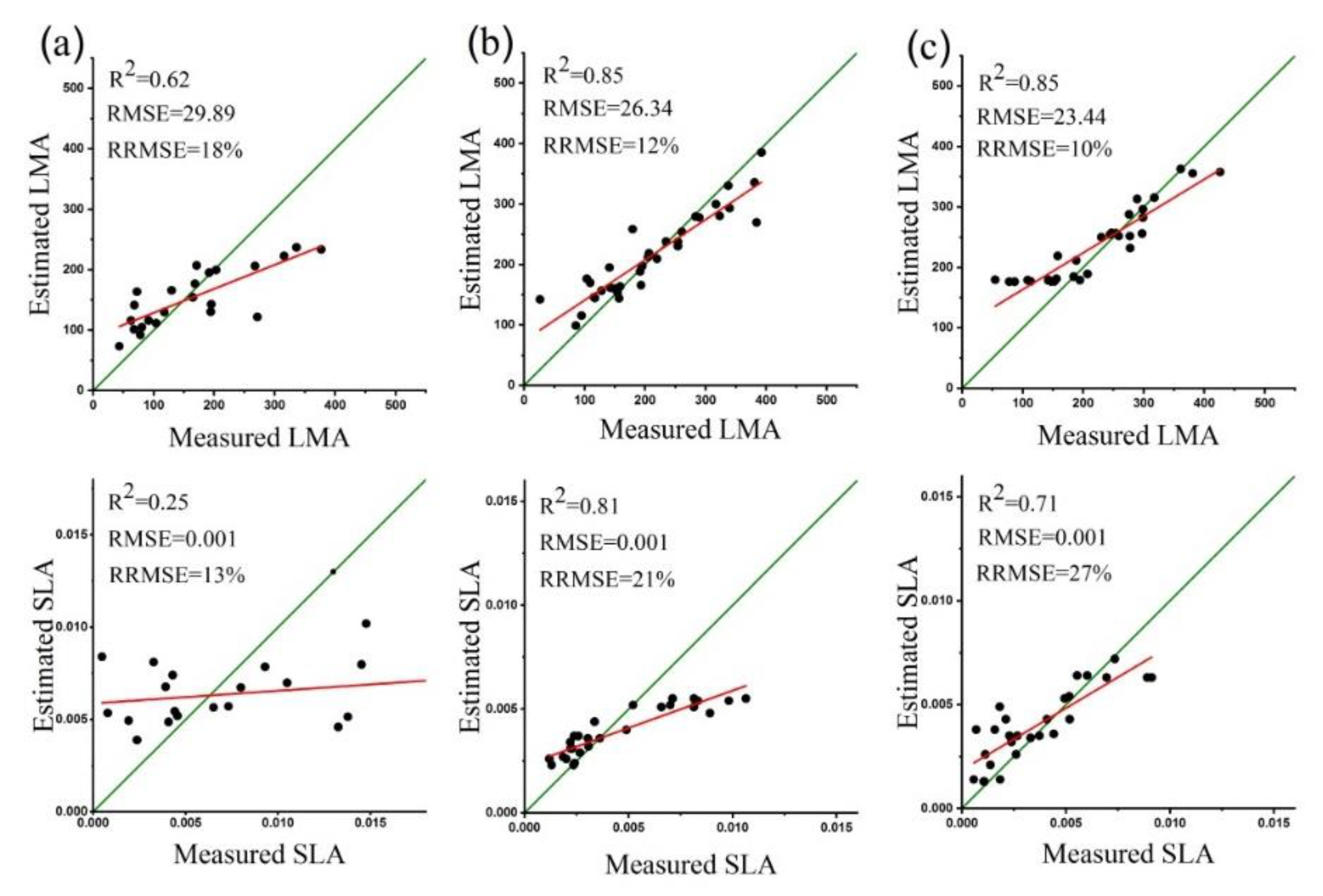
3.5. Estimation LMA and SLA using Spectral VIs

The performance of all the indices were compared at the different phenological stages to select the optimum index in the prediction of LAI and DW. The best-fit regression model illustrated the good relationship in the prediction of LAI and DW (Table 4 and Table 5), respectively, at nearly all growth stages, except the maturity stage, which was excluded from the data. The best-fit model equations of the optimal VIs were applied for the prediction of LAI and DW at each phenological stage and used in Equations (1) and (2) in the estimation of LMA and SLA, respectively. The spatial distributions of LAI, LMA and SLA are shown in Figures S2–S4. The optimal prediction equation was used in the LAI estimation, whereas LMA and SLA were utilised in Equations (1) and (2) for the generation of maps at all the explored phenological stages, respectively. Field measurement with the estimations from composited maps provided the validation results and illustrated the potential use of LAI, LMA and SLA derivation at all the growth stages.

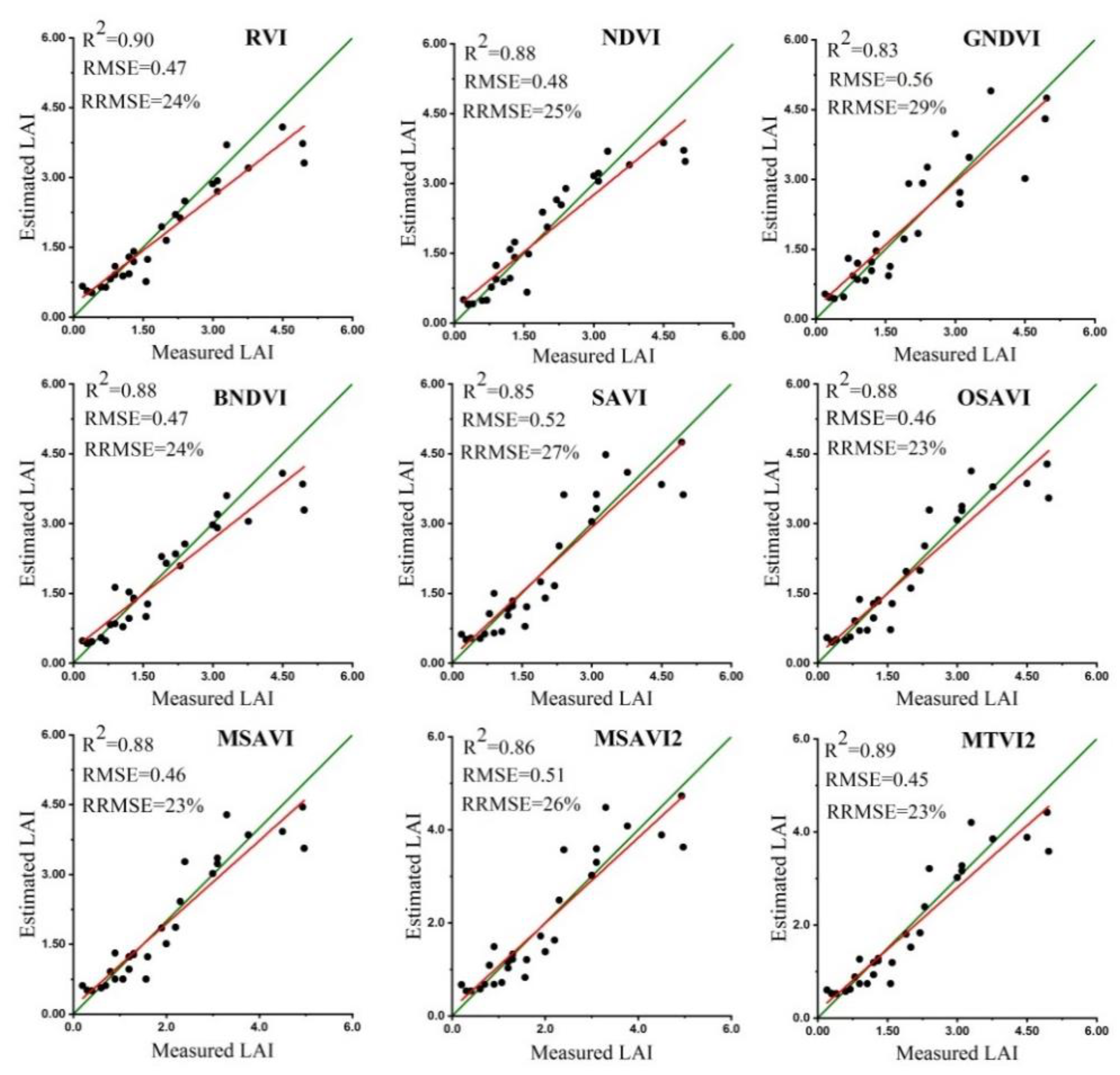
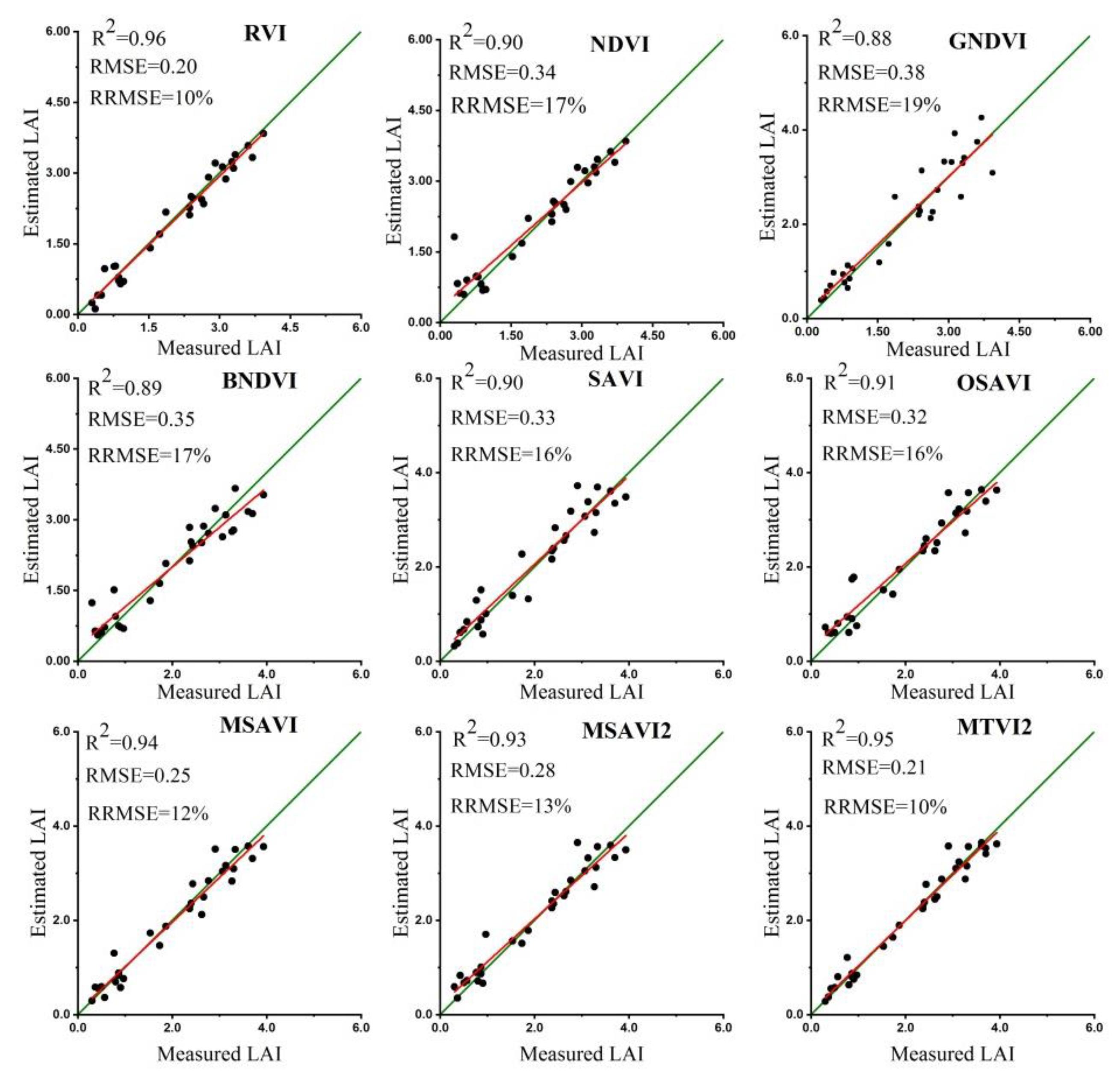
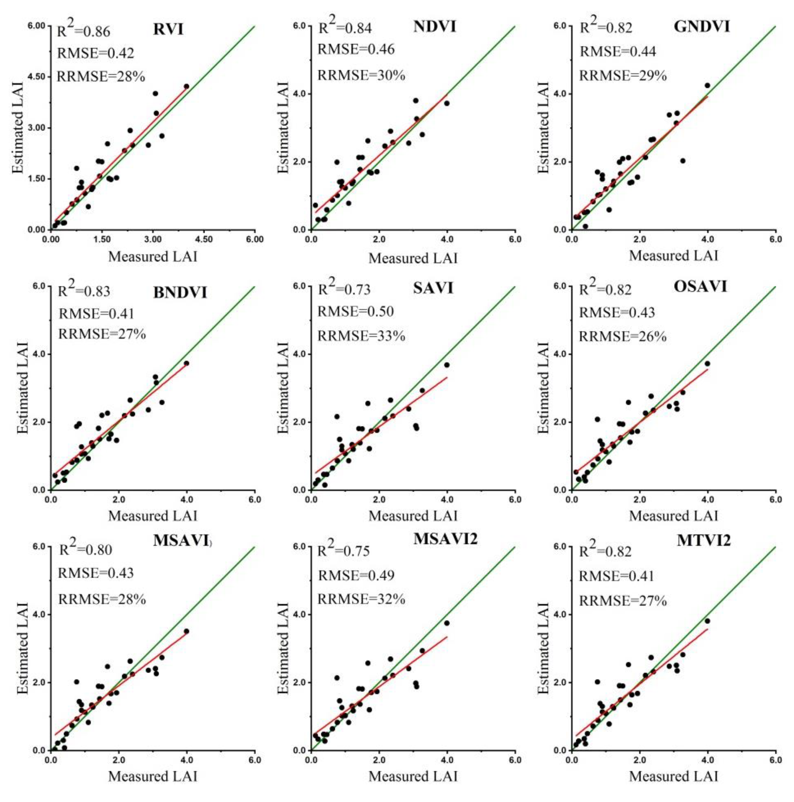
3.6. Validation of LAI, LMA and SLA Estimates

To validate the calibration model for LAI and estimated LMA, SLA with the predicted LAI and DW, multispectral images and ground measured data were used whilst the determined optimal VIs were considered in the prediction of LAI and DW at each growth stage and used in the estimation of LMA and SLA. The observed and estimated LAI, LMA and SLA were compared in Figure 3, Figure 4, Figure 5 and Figure 6. The predictions of optimal VIs were selected on the basis of the highest R² and lowest RMSE, which were plotted against the ground observed LAI, LMA and SLA. The optimal VIs, RVI and MTVI2 suggested consistency between the measured and estimated LAI (R² > 0.80) of rapeseed oil crops at all the growth stages. By contrast, the model validation demonstrated less adequate results for LMA and SLA at the seedling stage (R² = 0.62, 0.25) but realised consistent results at the elongation (R² = 0.85, 0.80) and flowering (R² = 0.85, 0.71) stages (Figure 6). Plotting the measured–estimated LMA values demonstrated less deviation from the 1:1 line, whereas SLA was strong under and over the prediction that occurs at higher SLA values, thereby suggesting the saturation of the spectral signal [46].

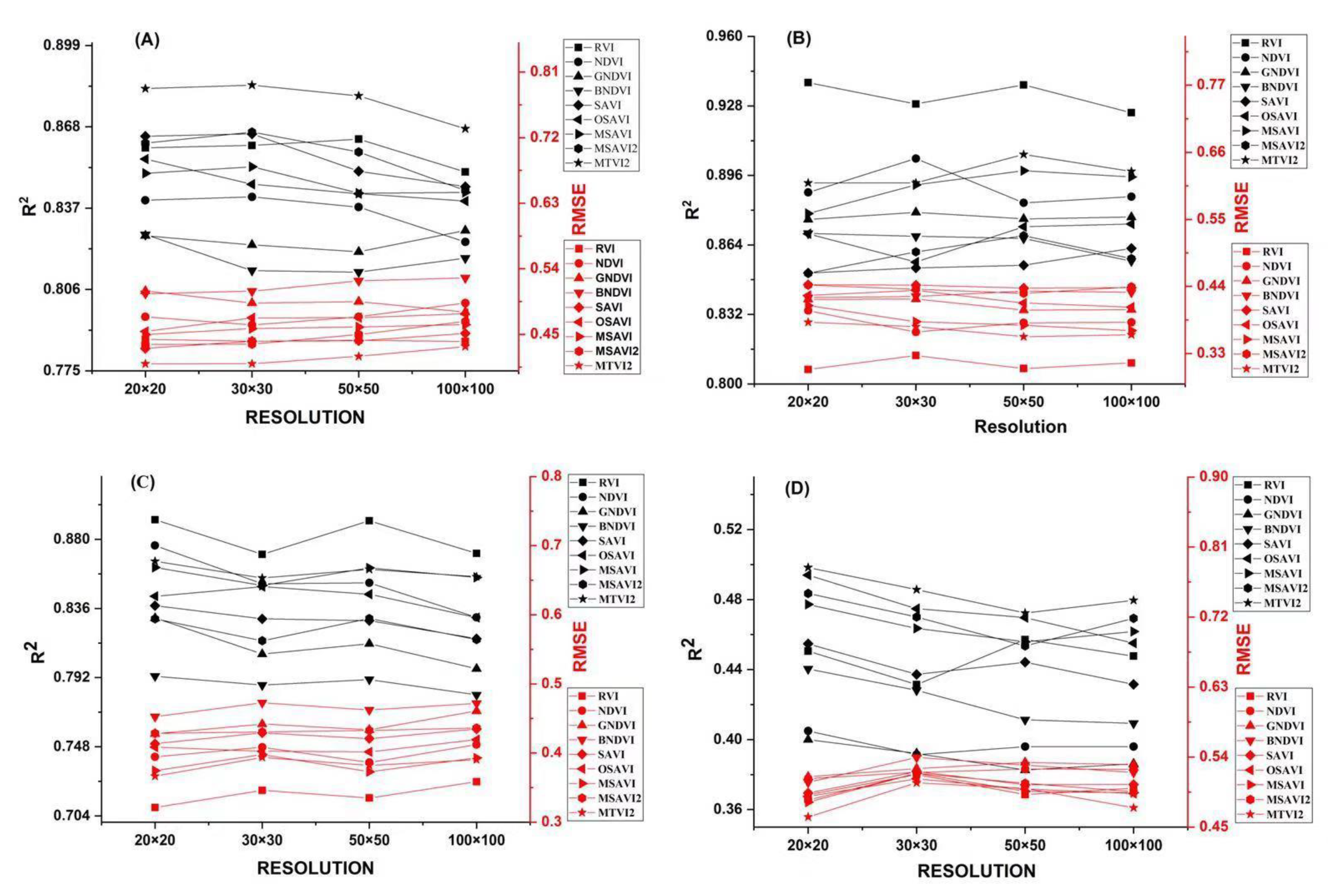
3.7. Evaluation of Image Resolution Effect

Four images with 20 cm pixel resolution were acquired over the rapeseed crops during the growing season and resampled to 30, 50 and 100 cm pixel resolutions. To evaluate the effects of image resolutions on the remote estimation of LAI over the rapeseed crops, the quantitative relationship between VIs and LAI were obtained at different image resolutions (20, 30, 50 and 100 cm). At all the mentioned image resolutions, the estimated LAI using VIs had no significant differences. The precision of the best-fit regression model between the LAI and VIs determined no significant variations and was similar at all the image resolutions. Thus, a significant high correlation between spectral VIs and LAI was acquired at the elongation and flowering stages, which are independent of image resolution. The best-fit model R² and RMSE are presented in Figure 7.

4. Discussion

As a remote sensing platform, UAVs are ideal for mapping and monitoring in PA [9,15]. With the recent developments in UAV technologies, numerous studies have been conducted using remote sensors onboard UAVs to evaluate its application for PA and subsequently obtained considerable attention from researchers [2,9,12,13,14,15,25,31,47].

The key canopy biophysical and biochemical parameter retrievals can be attained adequately using certain spectral bands, that is, the green spectrum is ideal for leaf chlorophyll estimation [35]. Reflectance in the near-infrared (NIR) is recognised as sensitive to variant biomass and canopy structures, whereas the red and green reflectance values respond to the background variations and senescent vegetation [48].

This study aimed to determine the optimal VIs derived from UAV multispectral images that could be used for the remote and empirical non-destructive estimation of biophysical parameters, such as LAI, LMA and SLA over rapeseed crops at the different growth stages. The empirical method for the estimation of biophysical parameters is proficient and delivers precise estimations [24,32]. Moreover, this type of method has been widely applied for the improved quantitative accuracy of spectral VIs and used for the evaluation of crop attributes, such as LAI, N status and biomass for various crops [10,49]. In this study, the potential capability of multispectral VIs mentioned in Table 1 was evaluated over rapeseed crops at different growth stages. The results revealed that the crop variations from seedling to maturity are similar to the canopy reflectance characteristics. Variations in the crop canopy reflectance attains its peak value at the elongation stage and begins to decline afterwards until the maturity stage; this behaviour is due to crop senescence, as reported previously in [10,50]. Variations in canopy reflectance at the different spectral wave bands are synchronised with LAI because of the modification of leaf chlorophyll contents at different phenological stages [51]. Spectral reflectance from the canopy is affected not only by the biophysical characteristics of foliage but also by the direction of incidence radiation, canopy architecture and soil background [52]. The small variations in spectral reflectance at the early phenological stage in the visible region are likely due to the crop nitrogen content and soil water background. However, variations in NIR reflectance with variant leaf orientations at certain growth stages are due to the overlapping leaves that decrease the active photosynthetic size as the LAI reaches a plateau [53,54].

Table 2 demonstrates the highly significant relationship between LAI with all the aforementioned spectral VIs derived from the multispectral remote sensing data. However, a close relationship was obtained by RVI with LAI because LAI had a value of approximately 3 m²m⁻², followed by NDVI and MTVI2 [55]. When LAI reached its saturation point, the reduced variability of red and NIR reflectance make RVI and NDVI insensitive. However, GNDVI apparently did not reach the saturation level even at LAI with moderate to high (4–5) values. The precision of the LAI estimate was better when green and blue bands were used instead of that that with the red band even at LAI values greater than 3 m²m⁻² [42]. The NIR band has a considerably strong impact on the relationship between LAI and spectral reflectance and must be considered under varying crop situations [7,10,56]. The nonlinear best-fit function between LAI and VIs demonstrated inconsistent sensitivity, and R² and RMSE values for estimating the accuracy of LAI can be misleading. Thus, the sensitivity analysis (NE) can be applied as the precision indicator to verify the performance of VIs in LAI estimation [57,58].

LMA and SLA are important in determining plant composition and eco-physiological characterisation [17,59,60,61,62]. Compared with the general empirical approach for the estimation of SLA, as reported in [32,48], its indirect estimation using the predicted LAI and DW illustrated highly significant retrieval accuracy. The SLA results showed remarkable variations between the different growth stages, as shown in Figure 6. The estimation results of SLA at the elongation and flowering stages are consistent with those of previously reported studies [63]. Soil background has less affected the correlation results as the data were captured at mature seedling (rosette) stage. The slight change in the performance of multispectral VIs from the UAV images could be awarded to the different viewing geometries and instrument spectral response functions [32].

Remotely sensed LMA (R² = 0.85, nRMSE= 0.10) and (R² = 0.85, nRMSE = 0.12) at the elongation and flowering stages was calculated with high estimation accuracy, as previously reported in [47]. The study estimated LMA using the LUT-based PROSAIL inversion method over the rapeseed crop. The LMA estimation results were also consistent with [19] who estimated LMA across a wide range of plant species through continuous wavelet analysis, and the study demonstrated remarkable implications in the prediction of dry matter content at the canopy level.

In terms of image resolution, our study concluded that the application of very fine-resolution remote sensing images does not reflect any significant difference. Thus, the fine-resolution images would not essentially increase the prediction accuracy of the regression model between LAI and spectral VIs. The precision of regression model between LAI and VIs did not change significantly by using images with different resolutions, as shown in Figure 7. The end users of UAV images need to consider the spatial, spectral and temporal resolutions and processing time for site-specific crop monitoring and management, as previously reported in [2,29,64,65,66].

5. Conclusions

In summary, herein we reported the application of multispectral sensors onboard UAV in acquiring images of rapeseed crops and retrieving their biophysical characteristics, such as LAI, LMA and SLA, throughout the phenological stages. The results revealed that the strongest relationship of spectral VIs was obtained in the elongation stage. The sensitivity analysis between LAI and VIs revealed that RVI, MSAVI and MTVI2 were the optimal VIs for LAI estimation. LMA and SLA results demonstrated the significant estimation accuracy by using the predicted leaf DW and LAI at the elongation and flowering stages, respectively. In terms of image resolutions, robust results can still be obtained when the maximum 100 cm resolution imagery is used for oil rapeseed crop characterisation. Therefore, high-altitude images will be preferred in obtaining a decreased number of images, which will significantly influence image acquisition and processing time.

Compared with earlier remote sensing platforms, the sensor onboard UAVs had the basic advantage of reaching the targeted site and acquiring very comprehensive information throughout the growing season. Unlike satellite- and aircraft-based remote sensing platforms, the UAV remote sensing platform demonstrated better operational advantages, such as the provision of high-spatial resolution imagery with low operational cost and near-real-time data acquisition. Although satellite data were limited because of temporal resolution, cloud cover, availability at the ideal time and the operational cost for high-resolution imagery, this technology has become an important tool for large area mapping and monitoring because of its distinctive capabilities in satellite remote sensing imagery that offers extensive information in a synoptic and frequent manner.

References

1. Turner, D.; Lucieer, A.; Watson, C. An Automated Technique for Generating Georectified Mosaics from Ultra-High Resolution Unmanned Aerial Vehicle (UAV) Imagery, Based on Structure from Motion (SfM) Point Clouds. Remote Sens. 2012, 4, 1392–1410. [Google Scholar] [CrossRef] [Green Version]
2. Vega, F.A.; Ramirez, F.C.; Saiz, M.P.; Rosua, F.O. ScienceDirect Multi-temporal imaging using an unmanned aerial vehicle for monitoring a sunflower crop. Biosyst. Eng. 2015, 132, 19–27. [Google Scholar] [CrossRef]
3. Zhang, C.; Kovacs, J.M. The application of small unmanned aerial systems for precision agriculture: A review. Precis. Agric. 2015, 13, 693–712. [Google Scholar] [CrossRef]
4. Tremblay, N.; Vigneault, P.; Bélec, C.; Fallon, E.; Bouroubi, M.Y. A comparison of performance between UAV and satellite imagery for N status assessment in corn. In Proceedings of the 12th International Conference on Precision Agriculture, Sacramento, CA, USA, 20–23 July 2014. [Google Scholar]
5. Hunt, E.R.; Daughtry, C.S.T.; Mirsky, S.B.; Hively, W.D. Remote sensing with unmanned aircraft systems for precision agriculture applications. In Proceedings of the 2013 Second International Conference on Agro-Geoinformatics (Agro-Geoinformatics), Fairfax, VA, USA, 12–16 August 2013. [Google Scholar]
6. Zhao, G.; Miao, Y.; Wang, H.; Su, M.; Fan, M.; Zhang, F.; Jiang, R.; Zhang, Z.; Liu, C.; Liu, P.; et al. A preliminary precision rice management system for increasing both grain yield and nitrogen use efficiency. Field Crops Res. 2013, 154, 23–30. [Google Scholar] [CrossRef]
7. Hatfield, J.L.; Prueger, J.H. Value of Using Different Vegetative Indices to Quantify Agricultural Crop Characteristics at Different Growth Stages under Varying Management Practices. Remote Sens. 2010, 2, 562–578. [Google Scholar] [CrossRef] [Green Version]
8. Warren, G.; Metternicht, G. Agricultural Applications of High-Resolution Digital Multispectral Imagery: Evaluating Within-Field Spatial Variability of Canola (Brassica napus) in Western Australia. Photogramm. Eng. Remote Sens. 2005, 71, 595–602. [Google Scholar] [CrossRef]
9. Primicerio, J.; Di Gennaro, S.F.; Fiorillo, E.; Genesio, L.; Lugato, E.; Matese, A.; Vaccari, F.P. A flexible unmanned aerial vehicle for precision agriculture. Precis. Agric. 2012, 13, 517–523. [Google Scholar] [CrossRef]
10. Din, M.; Zheng, W.; Rashid, M.; Wang, S.; Shi, Z. Evaluating Hyperspectral Vegetation Indices for Leaf Area Index Estimation of Oryza sativa L. at Diverse Phenological Stages. Front. Plant Sci. 2017, 8, 1–17. [Google Scholar] [CrossRef] [Green Version]
11. Lan, Y.; Thomson, S.J.; Huang, Y.; Hoffmann, W.C.; Zhang, H. Current status and future directions of precision aerial application for site-specific crop management in the USA. Comput. Electron. Agric. 2010, 74, 34–38. [Google Scholar] [CrossRef] [Green Version]
12. Hunt, E.-R.; Horneck, D.; Gadler, D.; Bruce, A.; Turner, R.; Spinelli, C.; Brungardt, J.; Hamm, P. Detection of nitrogen deficiency in potatoes using small unmanned aircraft systems. In Proceedings of the 12th International Conference on Precision Agriculture, Sacramento, CA, USA, 20–23 July 2014. [Google Scholar]
13. Swain, K.C.; Zaman, Q.U. Rice Crop Monitoring with Unmanned Helicopter Remote Sensing Images. In Remote Sensing of Biomass—Principles and Applications; Fatoyinbo, T., Ed.; InTech: Rijeca, Croatia, 2012; pp. 253–272. [Google Scholar]
14. Laliberte, A. Unmanned aerial vehicle-based remote sensing for rangeland assessment, monitoring, and management. J. Appl. Remote Sens. 2009, 3, 033542. [Google Scholar] [CrossRef]
15. Lelong, C.; Burger, P.; Jubelin, G.; Roux, B.; Labbé, S.; Baret, F. Assessment of Unmanned Aerial Vehicles Imagery for Quantitative Monitoring of Wheat Crop in Small Plots. Sensors 2008, 8, 3557–3585. [Google Scholar] [CrossRef] [PubMed]
16. Tilman, D. Functional Diversity. In Encyclopedia of Biodiversity; Elsevier: Amsterdam, The Netherlands, 2001; Volume 3, pp. 109–120. [Google Scholar] [CrossRef]
17. Ali, A.M.; Darvishzadeh, R.; Skidmore, A.K.; van Duren, I.; Heiden, U.; Heurich, M. Prospect inversion for indirect estimation of leaf dry matter content and specific leaf area. Int. Arch. Photogramm. Remote Sens. Spat. Inf. Sci. 2015, 40, 277–284. [Google Scholar] [CrossRef] [Green Version]
18. Jin, X.; Diao, W.; Xiao, C.; Wang, F.; Chen, B.; Wang, K.; Li, S. Estimation of Wheat Agronomic Parameters using New Spectral Indices. PLoS ONE 2013, 8, e72736. [Google Scholar] [CrossRef] [PubMed] [Green Version]
19. Cheng, T.; Rivard, B.; Sánchez-Azofeifa, A.G.; Féret, J.-B.; Jacquemoud, S.; Ustin, S.L. Deriving leaf mass per area (LMA) from foliar reflectance across a variety of plant species using continuous wavelet analysis. ISPRS J. Photogramm. Remote Sens. 2014, 87, 28–38. [Google Scholar] [CrossRef]
20. De Riva, E.G.; Olmo, M.; Poorter, H.; Ubera, J.L.; Villar, R. Leaf Mass per Area (LMA) and Its Relationship with Leaf Structure and Anatomy in 34 Mediterranean Woody Species along a Water Availability Gradient. PloS ONE 2016, 11, 1–18. [Google Scholar] [CrossRef] [Green Version]
21. Homolova, L.; Malenovsky, Z.; Clevers, J.G.P.W.; Garcı´a-Santos, G. Review of optical-based remote sensing for plant trait mapping. Ecol. Complex. 2013, 15, 1–16. [Google Scholar] [CrossRef] [Green Version]
22. Wei, Z.; Zhang, B.; Liu, Y.; Xu, D. The Application of a Modified Version of the SWAT Model at the Daily Temporal Scale and the Hydrological Response unit Spatial Scale: A Case Study Covering an Irrigation District in the Hei River Basin. Water 2018, 10, 1064. [Google Scholar] [CrossRef] [Green Version]
23. Singh, G.; Saraswat, D. Development and evaluation of targeted marginal land mapping approach in SWAT model for simulating water quality impacts of selected second generation biofeedstock. Environ. Model. Softw. 2016, 81, 26–39. [Google Scholar] [CrossRef] [Green Version]
24. Xie, Q.; Huang, W.; Liang, D.; Chen, P.; Wu, C.; Yang, G.; Zhang, J.; Huang, L.; Zhang, D. Leaf area index estimation using vegetation indices derived from airborne hyperspectral images in winter wheat. IEEE J. Sel. Top. Appl. Earth Obs. Remote Sens. 2014, 7, 3586–3594. [Google Scholar] [CrossRef]
25. Viña, A.; Gitelson, A.A.; Nguy-Robertson, A.L.; Peng, Y. Comparison of different vegetation indices for the remote assessment of green leaf area index of crops. Remote Sens. Environ. 2011, 115, 3468–3478. [Google Scholar]
26. Marques, P.; Martins, M.; Baptista, A.; Torres, J.P.N. Communication Antenas for UAVs. J. Eng. Sci. Technol. Rev. 2018, 11, 90–102. [Google Scholar] [CrossRef]
27. Hardin, P.J.; Hardin, T.J. Small-Scale Remotely Piloted Vehicles in Environmental Research. Geogr. Compass 2010, 4, 1297–1311. [Google Scholar] [CrossRef]
28. Taylor, J.A.; Jacob, F.; Galleguillos, M.; Prévot, L.; Guix, N.; Lagacherie, P. The utility of remotely-sensed vegetative and terrain covariates at different spatial resolutions in modelling soil and watertable depth (for digital soil mapping). Geoderma 2013, 193–194, 83–93. [Google Scholar] [CrossRef]
29. Xu, Y.; Smith, S.E.; Grunwald, S.; Abd-Elrahman, A.; Wani, S.P. Evaluating the effect of remote sensing image spatial resolution on soil exchangeable potassium prediction models in smallholder farm settings. J. Environ. Manag. 2017, 200, 423–433. [Google Scholar] [CrossRef]
30. Kim, J.; Grunwald, S.; Rivero, R.G. Soil Phosphorus and Nitrogen Predictions Across Spatial Escalating Scales in an Aquatic Ecosystem Using Remote Sensing Images. IEEE Trans. Geosci. Remote Sens. 2014, 52, 6724–6737. [Google Scholar]
31. Vergara-Díaz, O.; Zaman-Allah, M.A.; Masuka, B.; Hornero, A.; Zarco-Tejada, P.; Prasanna, B.M.; Cairns, J.E.; Araus, J.L. A Novel Remote Sensing Approach for Prediction of Maize Yield Under Different Conditions of Nitrogen Fertilization. Front. Plant Sci. 2016, 7, 1–13. [Google Scholar]
32. Liu, S.; Li, L.; Gao, W.; Zhang, Y.; Liu, Y.; Wang, S.; Lu, J. Diagnosis of Nitrogen Status In Winter Oilseed Rape (Brassica napus L.) Using In-situ Hyperspectral Data and Unmanned Aerial Vehicle (UAV) Multispectral Images. Comput. Electron. Agric. 2018, 151, 185–195. [Google Scholar] [CrossRef]
33. Pearson, R.L.; Miller, L.D. Remote Mapping of Standing Crop Biomass for Estimation of the Productivity of the Shortgrass Prairie; Colorado State University: Fort Collins, CO, USA, 1972. [Google Scholar]
34. J Rouse, J.W.; Haas, R.W.; Schell, J.A.; Deering, D.H.; Harlan, J.C. Monitoring the Vernal Advancement and Retrogradation (Greenwave effect) of Natural Vegetation; NASA/GSFC: Greenbelt, MD, USA, 1974.
35. Gitelson, A.A.; Kaufman, Y.J.; Merzlyak, M.N. Use of a green channel in remote sensing of global vegetation from EOS-MODIS. Remote Sens. Environ. 1996, 58, 289–298. [Google Scholar] [CrossRef]
36. Wang, F.M.; Huang, J.F.; Tang, Y.L.; Wang, X.Z. New Vegetation Index and Its Application in Estimating Leaf Area Index of Rice. Rice Sci. 2007, 14, 195–203. [Google Scholar] [CrossRef]
37. Huete, A. A soil-adjusted vegetation index (SAVI). Remote Sens. Environ. 1988, 25, 295–309. [Google Scholar] [CrossRef]
38. Haboudane, D. Hyperspectral vegetation indices and novel algorithms for predicting green LAI of crop canopies: Modeling and validation in the context of precision agriculture. Remote Sens. Environ. 2004, 90, 337–352. [Google Scholar] [CrossRef]
39. Rondeaux, G.; Steven, M.; Baret, F. Optimization of soil-adjusted vegetation indices. Remote Sens. Environ. 1996, 55, 95–107. [Google Scholar] [CrossRef]
40. Whiting, M.L.; Ustin, S.L.; Zarco-Tejada, P.; Palacios-Orueta, A.; Vanderbilt, V.C. Hyperspectral mapping of crop and soils for precision agriculture. In Remote Sensing and Modeling of Ecosystems for Sustainability III; Gao, W., Ustin, S.L., Eds.; SPIE: Bellingham, WA, USA, 2006; Volume 6298, p. 62980B. [Google Scholar]
41. Qi, J.; Chehbouni, A.; Huete, A.R.; Keer, Y.H.; Sorooshian, S. A modified soil adusted vegetation index. Remote Sens. Environ. 1994, 48, 119–126. [Google Scholar] [CrossRef]
42. Li, F.; Mao, L.; Hennig, S.D.; Gnyp, M.L.; Chen, X.P.; Jia, L.L.; Bareth, G. Evaluating hyperspectral vegetation indices for estimating nitrogen concentration of winter wheat at different growth stages. Precis. Agric. 2010, 11, 335–357. [Google Scholar] [CrossRef]
43. Din, M.; Ming, J.; Hussain, S.; Ata-Ul-Karim, S.T.; Rashid, M.; Tahir, M.N.; Hua, S.; Wang, S. Estimation of dynamic canopy variables using hyperspectral derived vegetation indices under varying N rates at diverse phenological stages of rice. Front. Plant Sci. 2019, 9, 1–16. [Google Scholar] [CrossRef] [Green Version]
44. Taylor, P.; Gitelson, A.A. Remote estimation of crop fractional vegetation cover : the use of noise equivalent as an indicator of performance of vegetation indices. Int. J. Remote Sens. 2013, 34, 37–41. [Google Scholar]
45. Nguy-Robertson, A.L.; Peng, Y.; Gitelson, A.A.; Arkebauer, T.J.; Pimstein, A.; Herrmann, I.; Karnieli, A.; Rundquist, D.C.; Bonfil, D.J. Estimating green LAI in four crops: Potential of determining optimal spectral bands for a universal algorithm. Agric. For. Meteorol. 2014, 192–193, 140–148. [Google Scholar] [CrossRef]
46. Roelofsen, H.D.; Van Bodegom, P.M.; Kooistra, L.; Witte, J.P.M. Predicting leaf traits of herbaceous species from their spectral characteristics. Ecol. Evol. 2014, 4, 706–719. [Google Scholar] [CrossRef]
47. Wang, S.Q.; Gao, W.H.; Ming, J.; Li, L.T.; Xu, D.H.; Liu, S.S.; Lu, J.W. A TPE based inversion of PROSAIL for estimating canopy biophysical and biochemical variables of oilseed rape. Comput. Electron. Agric. 2018, 152, 350–362. [Google Scholar] [CrossRef]
48. Houborg, R.; Anderson, M.; Daughtry, C. Utility of an image-based canopy reflectance modeling tool for remote estimation of LAI and leaf chlorophyll content at the field scale. Remote Sens. Environ. 2009, 113, 259–274. [Google Scholar] [CrossRef]
49. Li, F.; Mistele, B.; Hu, Y.; Chen, X.; Schmidhalter, U. Comparing hyperspectral index optimization algorithms to estimate aerial N uptake using multi-temporal winter wheat datasets from contrasting climatic and geographic zones in China and Germany. Agric. For. Meteorol. 2013, 180, 44–57. [Google Scholar] [CrossRef]
50. Xiong, D.; Wang, D.; Liu, X.; Peng, S.; Huang, J.; Li, Y. Leaf density explains variation in leaf mass per area in rice between cultivars and nitrogen treatments. Ann. Bot. 2016, 117, 963–971. [Google Scholar] [CrossRef] [PubMed] [Green Version]
51. Jégo, G.; Pattey, E.; Liu, J. Using Leaf Area Index, retrieved from optical imagery, in the STICS crop model for predicting yield and biomass of field crops. Field Crops Res. 2012, 131, 63–74. [Google Scholar]
52. Carvalho, S.; Van der Putten, W.H.; Hol, W.H.G. The Potential of Hyperspectral Patterns of Winter Wheat to Detect Changes in Soil Microbial Community Composition. Front. Plant Sci. 2016, 7, 1–11. [Google Scholar] [CrossRef] [Green Version]
53. Huang, M.; Yang, C.; Ji, Q.; Jiang, L.; Tan, J.; Li, Y. Tillering responses of rice to plant density and nitrogen rate in a subtropical environment of southern China. Field Crops Res. 2013, 149, 187–192. [Google Scholar] [CrossRef]
54. Tian, Y.-C.; Yang, J.; Yao, X.; Zhu, Y.; Cao, W.-X. Quantitative relationships between hyper-spectral vegetation indices and leaf area index of rice. J. Appl. Ecol. 2009, 20, 1685–1690. [Google Scholar]
55. Zhang, F.; Zhou, G.; Nilsson, C. Remote estimation of the fraction of absorbed photosynthetically active radiation for a maize canopy in Northeast China. J. Plant Ecol. 2015, 8, 429–435. [Google Scholar] [CrossRef] [Green Version]
56. Darvishzadeh, R.; Atzberger, C.; Skidmore, A.K.; Abkar, A.A. Leaf Area Index derivation from hyperspectral vegetation indicesand the red edge position. Int. J. Remote Sens. 2009, 30, 6199–6218. [Google Scholar] [CrossRef]
57. Xiao, Y.; Zhao, W.; Zhou, D.; Gong, H. Sensitivity Analysis of Vegetation Reflectance to Biochemical and Biophysical Variables at Leaf, Canopy, and Regional Scales. IEEE Trans. Geosci. Remote Sens. 2014, 52, 4014–4024. [Google Scholar] [CrossRef]
58. Marshall, M.; Thenkabail, P.; Biggs, T.; Post, K. Hyperspectral narrowband and multispectral broadband indices for remote sensing of crop evapotranspiration and its components (transpiration and soil evaporation). Agric. For. Meteorol. 2016, 218–219, 122–134. [Google Scholar] [CrossRef] [Green Version]
59. Reich, P.B.; Ellsworth, D.S.; Walters, M.B. Leaf structure (specific leaf area) modulates photosynthesis–nitrogen relations : Evidence from within and across species and functional groups. Funct. Ecol. 1998, 12, 948–958. [Google Scholar] [CrossRef]
60. Nautiyal, P.C.; Rao, N.; Joshi, Y.C. Moisture-deficit-induced changes in leaf-water content, leaf carbon exchange rate and biomass production in groundnut cultivars differing in specific leaf area. Field Crops Res. 2002, 74, 67–79. [Google Scholar] [CrossRef]
61. Vergara-díaz, O.; Zaman-allah, M.A.; Masuka, B.; Hornero, A. A Novel Remote Sensing Approach for Prediction of Maize Yield Under Different Conditions of Nitrogen Fertilization. Front. Plant Sci. 2016, 7, 1–13. [Google Scholar]
62. Li, C.; Wulf, H.; Schmid, B.; He, J.; Schaepman, M.E.; Member, S. Estimating Plant Traits of Alpine Grasslands on the Qinghai-Tibetan Plateau Using Remote Sensing. IEEE J. Sel. Top. Appl. Earth Obs. Remote Sens. 2018, 11, 1–13. [Google Scholar] [CrossRef]
63. Anser, G.P.; Martin, R.E. Airborne spectranomics : mapping canopy chemical and taxonomic diversity in tropical forests. Environ. Front. Ecol. 2009, 7, 269–276. [Google Scholar]
64. Myneni, R.B.; Williams, D.L. On the relationship between FAPAR and NDVI. Remote Sens. Environ. 1994, 49, 200–211. [Google Scholar] [CrossRef]
65. Steinberg, A.; Chabrillat, S.; Stevens, A.; Segl, K.; Foerster, S. Prediction of common surface soil properties based on Vis-NIR airborne and simulated EnMAP imaging spectroscopy data: Prediction accuracy and influence of spatial resolution. Remote Sens. 2016, 8, 613. [Google Scholar] [CrossRef] [Green Version]
66. Maynard, J.J.; Johnson, M.G. Scale-dependency of LiDAR derived terrain attributes in quantitative soil-landscape modeling: Effects of grid resolution vs. neighborhood extent. Geoderma 2014, 230–231, 29–40. [Google Scholar] [CrossRef] [Green Version]
Figure 1. Zishi experimental station and field view.
Remotesensing 12 00397 g001
Figure 2. Sensitivity analysis for VIs evaluated for LAI estimation.
Remotesensing 12 00397 g002
Figure 3. Estimated vs. measured LAI at the seedling stage. The green line shows the 1:1 correlation of the estimated and measured variables, whereas the red lines present the linear regression models.
Remotesensing 12 00397 g003
Figure 4. Estimated vs. measured LAI at the elongation stage. The green line shows the 1:1 correlation of the estimated and measured variables, whereas the red lines present the linear regression models.
Remotesensing 12 00397 g004
Figure 5. Estimated vs. measured LAI at the flowering stage. The green line shows the 1:1 correlation of the estimated and measured variables, whereas the red lines represent the linear regression models.
Remotesensing 12 00397 g005
Figure 6. Estimated vs. measured LMA and SLA at the (a) seedling, (b) elongation and (c) flowering stages. The green line shows the 1:1 correlation of the estimated and measured variables, whereas the red lines are the linear regression models.
Remotesensing 12 00397 g006
Figure 7. Best-fit model R2 and RMSE that describe the relationship between spectral VIs and LAI with respect to the image resolution at the (a) seedling, (b) elongation, (c) flowering and (d) maturity stages.
Remotesensing 12 00397 g007