Article

Quantitative Landscape Assessment Using LiDAR and Rendered 360° Panoramic Images

by
Rafał Wróżyński
1,*,
Krzysztof Pyszny
2 and
Mariusz Sojka
1
1
Institute of Land Improvement, Environmental Development and Geodesy, Faculty of Environmental Engineering and Spatial Management, Poznań University of Life Sciences, Piątkowska 94, 60-649 Poznań, Poland
2
EnviMap, ul. Piątkowska 118/31, 60-649 Poznań, Poland
*
Author to whom correspondence should be addressed.
Remote Sens. 2020, 12(3), 386; https://doi.org/10.3390/rs12030386
Submission received: 23 December 2019 / Revised: 15 January 2020 / Accepted: 23 January 2020 / Published: 25 January 2020

Abstract

:
The study presents a new method for quantitative landscape assessment. The method uses LiDAR data and combines the potential of GIS (ArcGIS) and 3D graphics software (Blender). The developed method allows one to create Classified Digital Surface Models (CDSM), which are then used to create 360° panoramic images from the point of view of the observer. In order to quantify the landscape, 360° panoramic images were transformed to the Interrupted Sinusoidal Projection using G.Projector software. A quantitative landscape assessment is carried out automatically with the following landscape classes: ground, low, medium, and high vegetation, buildings, water, and sky according to the LiDAR 1.2 standard. The results of the analysis are presented quantitatively—the percentage distribution of landscape classes in the 360° field of view. In order to fully describe the landscape around the observer, graphs of little planets have been proposed to interpret the obtained results. The usefulness of the developed methodology, together with examples of its application and the way of presenting the results, is described. The proposed Quantitative Landscape Assessment method (QLA360) allows quantitative landscape assessment to be performed in the 360° field of view without the need to carry out field surveys. The QLA360 uses LiDAR American Society of Photogrammetry and Remote Sensing (ASPRS) classification standards, which allows one to avoid differences resulting from the use of different algorithms for classifying images in semantic segmentation. The most important advantages of the method are as follows: observer-independent, 360° field of view which simulates human perspective, automatic operation, scalability, and easy presentation and interpretation of results.

Graphical Abstract

1. Introduction

The landscape plays an important role in the cultural, ecological, environmental, and social fields. Landscape is an important element of the quality of life of people all over the world, both for urban and countryside inhabitants [1]. Landscape analysis plays a key role in research on urban ecology [2], urban planning [3], urban heat island studies [4], and monitoring of landscape changes [5]. The procedures for landscape identification and assessment should be based on the exchange of experience and methodology.
The interest in landscape research increased significantly at the beginning of the 21st century. Dynamic progress of Geographic Information Systems (GIS) and widespread availability of high-resolution data contributed to the development of many methods used for landscape assessment. Among the methods developed so far, two are the most frequently used. The first one is based on spatial data analyses, which describe the landscape compositions and patterns in the form of 2D categorical maps [6,7]. The second one is based on eye-level photographs, and the landscape is characterized either by qualitative questionnaire surveys [8,9,10,11] or quantitative computer vision and machine learning algorithms [12,13].
The 2D categorical maps can be made with a series of developed metrics that can effectively characterize landscape structures, but they can be misleading when correlated with people’s 3D visual landscape preferences [14] because of the lack of quantitative information in the vertical direction [15]. The availability of high-resolution Digital Elevation Models (DEMs), Digital Surface Models (DSMs), and LiDAR point clouds allowed for the generation of 3D models [16,17,18] and the implementation of the third dimension to the analysis workflow in environmental modeling [19,20,21,22]. Although it greatly improved the quality of landscape classifications, it does not solve the biggest issue of landscape mapping, which is the potential discrepancy between landscape classification and the actual view from the observer location. The main problem with landscape classification mapping is the strict borders of adjacent classes. Zheng et al. [23] pointed out that the two most commonly used approaches, which are moving window and grid methods, takes groups of contiguous pixels as neighborhoods while overlooking the fact that ecological processes do not occur in fixed boundaries. In the moving window method, the results of landscape metrics are summarized in the central pixel of the window to construct a new metric map. On the other hand, the grid method subdivides a map with equal-size blocks. The same applies to the viewshed area of the observer, which is variable in different, sometimes very close locations (just around the corner). The fact that the observer sees only the first reflection of the surrounding environment makes the practical usefulness of landscape classification maps questionable.
From the observer point of view, the methods of landscape characterization using eye-level photographs seem to be more useful, as they try to simulate the perspective from the human eye instead of 2D maps. Visual assessment of landscapes and landscape elements has relied heavily on the use of photographs since the 1960s [24]. However, the lack of a uniform methodology of taking photos and making questionnaire surveys makes it difficult to compare the results from different studies. The basic factor, which is the camera focal length, varies in different studies and takes, for example, 38 [25], 50 [26], and 55 mm [27]. The sensor size is often undefined despite the fact that it is, together with the focal length value, crucial for defining the field of view (FOV). There are many factors that may influence the perception of landscape photographs during questionnaire surveys, such as image exposure, highlights, black point, hue, and saturation [28]. The composition of the landscape photo may unintentionally have a direct impact on the perception, as it is used by professional photographers to direct viewers’ attention to the intended focal point and yield a visually appealing image [29]. The issue related to the composition and unstandardized FOV can be resolved with the use of 360° panoramic images, which capture the whole scene surrounding the observer. Huge progress in computer vision and machine learning algorithms observed lately allowed for observer-independent image classification, which can be applied for landscape description [13,30,31]. Panoramic images from the Google Street View (GSV) database along with machine learning has proved to be useful for quantification of the landscape in an urban environment [32,33,34,35]; however, GSV image locations are biased towards streets and do not offer complete coverage of open areas at this point.
Simensen et al. [36], on the basis of a review of 54 contemporary landscape characterization approaches, stated that no single method can address all dimensions of the landscape without important trade-offs. Thus, there is still a need for quantitative, observer-independent methods for landscape characterization.
In this work, a landscape is defined as any permanent object in the human 360° field of view at a given location. This assumption meets the definition of a European Landscape Convention that defines a landscape as an area, as perceived by people, whose character is the result of the action and interaction of natural and/or human factors [1].
The aims of the study were to (1) develop a methodology of Quantitative Landscape Assessment (QLA360) from the perspective of an observer in the full 360° panoramic field of view and (2) demonstrate the practical applicability of the methodology. The following requirements were assumed at the stage of developing the method concept: observer-independent, 360° field of view, automatic operation, scalability, and easy presentation of results. The methodology is based on the data obtained from airborne laser scanning (LiDAR) and integrates the use of GIS and 3D graphics software.

2. Methodology

2.1. Data

The QLA360 is based on point clouds obtained from airborne laser scanning (LiDAR). The basic information contained in the point cloud are coordinates presenting the location in 3D space. Moreover, the RGB values, intensity, number of returns, and classification are attached to each point. The classes of point cloud in the LAS 1.2 format are shown in Table 1. The LiDAR data used in this study were obtained from the Polish Head Office of Land Surveying and Cartography. The surveying was done in July 2012. The mean spatial error of data was 0.08 m horizontal and 0.1 m vertical. The average density of a point cloud was 6.8 points per square meter. According to LiDAR data provider, the point cloud classification was carried out in TerraScan and TerraModeler modules of TerraSolid software according to the LAS 1.2 standard of the American Society of Photogrammetry and Remote Sensing (ASPRS) (Table 1). The classification was carried out in two stages. First, automatic classification was carried out using TerraSolid algorithms. Then a manual correction was made, which is a process of checking the effectiveness of the automatic classification and its completion in places where the automatic filtration process did not bring satisfactory results. The classification process is completed when the classification error is less than 5%. Six classes were used for landscape analysis: ground, low vegetation (height < 0.4 m), medium vegetation (height 0.4–2 m), high vegetation (height > 2 m), building, and water.

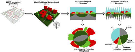
2.2. Classified Digital Surface Model (CDSM) Development

The QLA360 methodology assumes the inclusion of all objects within the sight range of the observer. The input data are the LiDAR point cloud and the observer’s locations (Figure 1).
The DSM in raster format was developed in 1 m resolution on the basis of a LiDAR point cloud. The observer location is a vector shapefile layer containing one or multiple points with X and Y coordinates and height 1.7 m above the ground level to simulate the line of sight [12]. The Viewshed tool identifies the areas that can be seen from one or multiple observer points. The result of the analysis was a raster map with a resolution of 1 m, where 0 means no visibility and 1 means visibility. Based on the results of the Viewshed analysis and by using the Minimum Bounding Geometry tool, an area of further analysis was determined (vector shape file—AoI.shp).
Using the AoI.shp file, the point cloud was clipped to an area that will be subject to further detailed analysis. From the clipped point cloud, points representing ground (2), low vegetation (3), medium vegetation (4), high vegetation (5), buildings (6), and water (9) were selected for separate layers. Then, based on point clouds, mesh files were created in the form of TIN (Triangulated Irregular Network). Mesh files allowed us to reconstruct the topography and low, medium, and high vegetation and buildings. The process of converting point clouds to meshes was conducted in CloudCompare v.2.1 (https://www.danielgm.net/cc/), which is an open-software project for 3D point cloud processing that provides a set of tools for managing and editing point clouds and triangular meshes [38]. The process consists of rasterization of the point cloud with specified resolution and then converting it to a mesh in the form of TIN. The process is relatively easy with the continuous ground mesh, but the automatic transformation of relatively sparse (4–12 points/m2) point clouds of objects above the ground level, which lack points on the sides, is a difficult task and can introduce some errors, especially in the case of vegetation. In this study, a simplified method was used in which the meshes were created on the basis of first returns of points in each class, and then they were extruded on the z-axis to the ground. This allowed for automation of the task and moreover, for correct representation of vertical features (building elevations) on the 3D model. All of the models were exported separately in the .fbx format.
In the next step, all of the developed models were imported into Blender Software v.2.79. Blender is a free and open-source 3D creation suite. It supports the entirety of the 3D pipeline—modeling, rigging, animation, simulation, rendering, compositing and motion tracking, video editing, and game creation. The great versatility of the program allows for performing a 3D visual impact analysis [39]. Blender’s scene consisting of a complete, natural scale, 3D model of the study site can be used to perform renders from any location.

2.3. 360° Panoramic Images Rendering

Blender uses the Cycles Render Engine, which is a ray tracing, physically-based production renderer used for creating photo-realistic images and animations. Rendering is the process of creating 2D images from a 3D scene. The final look of the image is dependent on four factors, which can be controlled by the user: a camera, lighting, object material, and various render settings, such as resolution, sampling, and light paths. Blender’s virtual camera was set to panoramic view, which captures the full 360° field of view from the location of the camera and uses the equirectangular transformation to store the result in the form of a rectangular .png image. The camera can be set in any location of the 3D space. For the purpose of this study, camera (observer) locations were specified in the ArcGIS software as the point vector shapefile. The shapefiles were imported to the Blender scene using the BlenderGIS addon (https://github.com/domlysz/BlenderGIS), and the height value was fixed at 1.7 m above the ground surface. The scene lighting was set as the default background with blue color imitating the sky. Having the separated models representing all classes allows for the simple assignment of materials (colors) to them. At this stage, it is possible to add new 3D objects with unique RGB material assigned, in order to perform visual impact analysis or to add objects that are not included in the LiDAR point cloud but are needed in landscape analysis. The final scene consisting of the CDSM resulted in combining meshes representing each class with different material of known RGB values (Table 2). In order to achieve images of solid colors only, all the Cycle Engine settings, such as shadows, reflections, and volume, were disabled. In order to automate the rendering for multiple locations, the Python script was developed in the Blender environment (Appendix A).

2.4. Presentation of the Outputs

The output of the QLA360 method is the set of equirectangular 360° panoramic images, including ground, low, medium, and high vegetation separately, buildings, water, and sky visible from the perspective of the observers of known locations. This gives a wide variety of result presentation possibilities. The equirectangular images can be directly used in Virtual Reality devices, which can be useful for subjective visual impact assessment by the observers. Moreover, the equirectangular renders can be easily converted to stereographic (little planet) projections, which can help to understand the direction and spatial distribution of landscape features from the human perspective. In order to quantify the amount of visible landscape features, 360° panoramic images have been transformed to the Interrupted Sinusoidal Projection, which is a type of Equal-Area projection [40]. For the transformation, the G.Projector software developed by the National Aeronautics and Space Administration (NASA) was used. In order to reduce the distortion to a minimum, the 10° Gores Interruption was applied. Next, the pixels of colors representing each class were counted in every image. As the different classes are represented with different colors (RGB values), the amount of landscape features can be quantified as the percentage of pixels representing different colors (classes). In this study, in order to automate the task, the pixels were counted using Python and the PIL library (Appendix B), but it can be done in most graphic editor software such as Photoshop or Gimp. Percentage quantities of landscape features can be joined to the observer location vector points as the attributes. The results can be presented as charts with a percentage distribution of landscape features or thematic maps showing the classes separately.

3. Results

The QLA360 methodology was tested in the example of the City of Poznań, Poland. In the first stage, on the basis of the LiDAR point cloud, a DSM was developed. Then, the viewshed analysis was carried out for the six example observer locations with the set height of 1.7 m above the ground (Figure 2a). On the basis of the viewshed analysis results, the minimum bounding geometry tool was used to create an AoI polygon. It has an area of 1.71 km2 and was used to limit the range of further analysis. The point cloud with assigned RGB color values (Figure 2b) and class values according to the LAS 1.2 standard (Figure 2c) was clipped to the AoI extent. Next, the points were extracted separately by their class values, converted to meshes in CloudCompare software, and imported to Blender software (Figure 2d). In Blender, the material was assigned for each mesh class (Figure 2e). Next, the CDSM created in Blender and observer locations were used for rendering the 360° panoramic images.
Renders were made as equirectangular images with the resolution of 10,000 × 5000 pixels for all analyzed observer locations. This resolution was selected on the basis of the analysis performed on a set of images rendered with different resolutions for a single location (Figure 3). The difference in the number of pixels representing particular classes was less than 0.005%, and the render time was 129 s. All renders were made on the PC with the following parameters: Intel(R) Core(TM) i7-8700K CPU with 48 GB RAM and NVIDIA GeForce GTX 1080Ti GPU.
Rendered panoramic images are shown in Figure 4a–f (right top corner). In order to perform visual verification, the GSV panoramas were downloaded, using the methodology presented by Gong et al. [32] (Figure 4a–f, left top corner). The rendered and GSV panoramic images were then overlaid with 50% transparency, and the lines presenting north, south, east, and west directions were added for easier interpretation (Figure 4, bottom). The obtained results indicate that the CDSM developed on the basis of the LiDAR point cloud in Blender represents the landscape elements visible from the perspective of the observer well. The discrepancies between the rendered and GSV panoramic images are mainly temporary elements, such as cars, people, and others. There are also some differences in landscape features, particularly with regard to low vegetation and the lack of billboards (Figure 4c) and street lamps (Figure 4a,c,d). Individual inconsistencies in the classification of objects were also identified; for example, the street lamp was classified as high vegetation (Figure 4f). Differences between panoramic images may result from different dates of LiDAR and GSV surveys. Moreover, the classification of the LiDAR point cloud in the LAS standard is characterized by the quality of classification at the level of not less than 95%. The analysis shows that 360° panoramic images created with the QLA360 method can be used as the basis for further analysis of the landscape assessment. In order for the rendered panoramic images to be useful for further quantitative analysis, it is necessary to transform them. This is due to large distortion in the upper and lower part of the panoramic images in the equirectangular projection. The panoramic images were transformed using an Interrupted Sinusoidal Projection from the Equal-Area projections group using G.Projector software developed by NASA. The results of the 360° panoramic images transformation are shown in Figure 5.
The transformed panoramic images were used for further calculations to determine the percentage distribution of each landscape feature in the entire 360° panoramic image. In order to automate the calculation process, a Python script was developed for counting pixels of different classes. It allowed us to calculate the percentage values of separated classes in accordance with the LAS 1.2. standard, which were shown as pie charts (Figure 6a). Additionally, the panoramic images were transformed into a stereographic projection, which enabled presentation of the results with so-called little planets (Figure 6b). In addition, the results can be presented independently for each landscape feature as low vegetation, medium vegetation, high vegetation (Figure 6c), buildings (Figure 6d), and sky.
Pie charts quantify the contribution of individual landscape elements. However, they do not fully show which elements of the landscape are in the immediate vicinity of the observer and to which extent they may dominate in the 360° FOV. The little planet charts, although not allowing the quantitative landscape assessment on their own, enable one to determine the impact of particular landscape elements on the observer depending on their size and distance. A comparison of little planet charts from GSV images and renders from the Blender environment is shown in Figure 7.
The QLA360 method allows for automatic visibility analysis for any number of locations in an area where LiDAR data is available. An exemplary analysis was carried out for 113 observer points located manually on streets and sidewalks at a distance of approximately 25 m. The results can be presented in the GIS environment for all separated landscape elements (Figure 8). The results can be useful in comparing the visual aspects of different areas and to complement the spatial planning process.
Imperfections resulting from the LiDAR point cloud can be corrected in the Blender environment. The next example shows the analysis carried out for an observer located near the lake (Figure 9a). A common problem with LiDAR is its poor representation of water (Figure 9b). This problem can be easily resolved by implementing the CDSM with a polygon representing the water surface (Figure 9c).
Working in the 3D environment of the Blender software makes it easy to add new objects that can be considered in the visual impact analysis. It can be very helpful for planning new infrastructure, expanding green infrastructure [41], planning decision support systems for smart cities [42,43], and for performing an environmental impact assessment of potential investments. For example, three potential buildings were added to the CDSM (Figure 10a) and assigned with a different material of known RGB values (Figure 10c). The analysis shows the visual impact of the new buildings on the observers located down the road. The mean visibility of the new buildings for eight observer locations equals 5.77% of the 360° field of view with a maximum of 9.71% for observer 3 (before Figure 10b and after Figure 10e building construction). A slightly different view is obtained by observer 7 where the buildings are visible from the side and mutually obscure each other (before Figure 10c and after Figure 10f building construction). The new buildings are not visible for observer 8, as they are obstructed by high vegetation. The average sum of the total buildings fraction increased from 7.09% to 12.8%.

4. Discussion

The QLA360 method is based entirely on the classified LiDAR point cloud and does not require any additional data or surveys. As it is highly observer-independent, it can be used in any geographic location in the world, where LiDAR data are available, and gives comparable results. The application of LiDAR ASPRS classification standards as landscape classes allows avoiding differences resulting from the application of different algorithms for classifying images in semantic segmentation. The methodology can be applied in any location, which enables a quantitative comparison of the landscape obtained in the various areas. So far, mapping with LiDAR is a newly emerging, expensive technology. Most large-scale scans have only been performed once. In the near future, when more LiDAR scans are available, landscape changes can easily be tracked using the proposed methodology.
Many recently developed landscape assessment methods use semantic segmentation [34,44,45,46], also called scene labeling, which refers to the process of assigning a semantic label (e.g., vegetation, buildings, and cars) to each pixel of an image. In the QLA360 methodology, the same results in the form of classified images are obtained. The use of standardized classification allows one to avoid differences resulting from the use of different algorithms for classifying images. The image segmentation methods are able to define landscape features on the photographs with high accuracy, but their wide applicability of landscape assessment can be limited by the high cost of field work for taking the photographs. The objective comparison of the results can also be an issue as these methods use different classification algorithms and there is a lack of standard methodology for obtaining the photographs. The use of 360° panoramic images can eliminate the problem with subjective framing of photographs and could be a way of standardizing the input data for semantic segmentation algorithms. The GSV is a database that can be successfully used in landscape assessment allowing a great number of input data to be obtained for analysis, eliminating the issue of taking photographs manually [34]. GSV image locations, however, do not cover every location as they are biased toward the streets at the moment. Our method allows one to generate one’s own panoramic images so they can be applied in any location regardless of the availability of GSV. Another problem to confront in semantic segmentation is the elimination of temporary objects (cars, people). The QLA360 method is based on the classified LiDAR point cloud, which is already filtered from temporary objects. Many different classifications of landscape features can be found in the literature (Table 3).
The definition of classes depends on the input data used. GSVs and photographs may contain more detailed classes, but their analysis is more difficult and time consuming. Our methodology, entirely based on LiDAR, will evolve along with the standards of point cloud classification. The methodology can be easily adapted to different LAS standards. The LAS 1.4 version additionally includes: railway, surface, wire, transmission, and bridge classes [50]. All these classes can be included in the analysis simply by assigning new, unique RGB material to them and slightly modifying the script (Appendix B) to include new classes in the pixel counting process. In addition to the LAS classification, the QLA360 allows implementing additional classes by assigning new RGB material to them. It can be used, for example, to differentiate buildings as public, private, historic, etc.
The proposed methodology can be useful for urban planners. Quantified results of visible landscape features can help maintain or restore balance between natural and anthropogenic features and can help to adapt the urban environment to people’s landscape preferences [14]. The presentation of the results in the form of stereographic projection—little planet diagrams—can be useful in urban planning as it shows the cumulation and direction of landscape features. Unlike methods based on image manipulation and photomontage, a visual impact assessment can be performed for many observer locations without additional effort. The implementation of the planned infrastructure into the photographs is time-consuming and requires appropriate skills, so in practice, no more than a few photomontages are performed from different perspectives [51]. The QLA360 method allows for integration of 3D models in the CDSM so it is possible to automatically generate a render with an appropriate scale and perspective from any number of observation sites. The result of the visual impact assessment is automatically generated in the quantified form of percentages in the observer’s field of view. This paper presents a simple example of implementing new buildings as basic 3D shapes, but it is possible to make an analysis for highly detailed 3D models of designed structures. It can also be used to assess the impact on the landscape by implementing new 3D models of vegetation. The generated equirectangular panoramic renders can be directly displayed with a virtual-reality head-set, which can be helpful for subjective evaluation of visual impact [52].
The use of LiDAR data also has certain limitations. The method of constructing the CDSM for the analysis consisting of meshing and extruding the first return of the object is simple, fast, user-independent, and does not require any additional data but can generate geometry errors and inaccuracies especially in the case of buildings and tree objects. The QLA360 method can be directly applied for already existing 3D city models with different Level of Detail (LOD), which can improve analysis results due to the better buildings geometry representation [53,54], and virtual environments made with game engines [55]. The reconstruction of individual trees is possible but requires a very high density LiDAR collected using UAV platforms [56,57] or Terrestrial Laser Scanning [58,59] or manually modeling vegetation in 3D modeling software. The versatility of the proposed methodology allows every object of the CDSM to be replaced with more detailed geometry when necessary.

5. Conclusions

The study shows great potential in extending GIS features with 3D graphic software and remote sensed data for landscape assessment. Presented methodology uses LiDAR point cloud as the only input data. It shows great versatility of LiDAR technology, as it is used for generating 3D models and, at the same time, divides generated objects by class. The classification of landscape features is directly adapted with ASPRS LAS classification, which makes the method observer-independent. As presented, the QLA360 method can be easily applied in the landscape impact assessment of new investments. The following detailed conclusions were reached:
  • The main advantages of the QLA360 method are: observer-independent, 360° field of view, automatic operation, scalability, and easy presentation and interpretation of results,
  • The QLA360 method allows for quantitative analysis of landscape elements from the perspective of an observer in the 360° field of view based on classified LIDAR point clouds,
  • A quantitative assessment of landscape features can be performed for any location without additional field studies,
  • The use of GIS tools and 3D graphics software in the QLA360 method allows to assess changes in the landscape caused by the introduction of new elements such as trees, buildings, and infrastructure,
  • The method is based on processed LIDAR point clouds developed in accordance with ASPRS standards; therefore, it allows for standardization of the classification of landscape features, gives comparable results, and can be easily applied in practice.

Author Contributions

Conceptualization, R.W.; methodology, R.W.; software, R.W.; investigation, R.W., K.P., M.S.; writing—original draft preparation, R.W., K.P., M.S.; writing—review and editing, R.W., K.P., M.S.; visualization, R.W.; supervision, R.W. All authors have read and agreed to the published version of the manuscript.

Funding

The publication was co-financed within the framework of the Ministry of Science and Higher Education programme as “Regional Initiative Excellence” in years 2019-2022, Project No. 005/RID/2018/19.

Conflicts of Interest

The authors declare no conflict of interest. The funders had no role in the design of the study; in the collection, analyses, or interpretation of data; in the writing of the manuscript, or in the decision to publish the results.

Appendix A

Remotesensing 12 00386 i001

Appendix B

Remotesensing 12 00386 i002

References

  1. Council of Europe. Council of European Landscape Convention, Florence, Explanatory Report. CETS No. 176; Council of Europe: Strasbourg, France, 2000. [Google Scholar]
  2. Aronson, M.F.J.; Lepczyk, C.A.; Evans, K.L.; Goddard, M.A.; Lerman, S.B.; MacIvor, J.S.; Nilon, C.H.; Vargo, T. Biodiversity in the city: Key challenges for urban green space management. Front. Ecol. Environ. 2017, 15, 189–196. [Google Scholar] [CrossRef] [Green Version]
  3. Badach, J.; Raszeja, E. Developing a framework for the implementation of landscape and greenspace indicators in sustainable urban planning. Waterfront landscape management: Case studies in Gdańsk, Poznań and Bristol. Sustainability 2019, 11, 2291. [Google Scholar] [CrossRef] [Green Version]
  4. Estoque, R.C.; Murayama, Y.; Myint, S.W. Effects of landscape composition and pattern on land surface temperature: An urban heat island study in the megacities of Southeast Asia. Sci. Total Environ. 2017, 577, 349–359. [Google Scholar] [CrossRef] [PubMed]
  5. Houet, T.; Verburg, P.H.; Loveland, T.R. Monitoring and modelling landscape dynamics. Landsc. Ecol. 2010, 25, 163–167. [Google Scholar] [CrossRef] [Green Version]
  6. De Vries, S.; Buijs, A.E.; Langers, F.; Farjon, H.; Van Hinsberg, A.; Sijtsma, F.J. Measuring the attractiveness of Dutch landscapes: Identifying national hotspots of highly valued places using Google Maps. Appl. Geogr. 2013, 45, 220–229. [Google Scholar] [CrossRef]
  7. Walz, U.; Stein, C. Indicator for a monitoring of Germany’s landscape attractiveness. Ecol. Indic. 2018, 94, 64–73. [Google Scholar] [CrossRef]
  8. Hedblom, M.; Hedenås, H.; Blicharska, M.; Adler, S.; Knez, I.; Mikusiński, G.; Svensson, J.; Sandström, S.; Sandström, P.; Wardle, D.A. Landscape perception: Linking physical monitoring data to perceived landscape properties. Landsc. Res. 2019, 00, 1–14. [Google Scholar] [CrossRef] [Green Version]
  9. Olszewska, A.A.; Marques, P.F.; Ryan, R.L.; Barbosa, F. What makes a landscape contemplative? Environ. Plan. B Urban Anal. City Sci. 2018, 45, 7–25. [Google Scholar] [CrossRef]
  10. White, M.; Smith, A.; Humphryes, K.; Pahl, S.; Snelling, D.; Depledge, M. Blue space: The importance of water for preference, affect, and restorativeness ratings of natural and built scenes. J. Environ. Psychol. 2010, 30, 482–493. [Google Scholar] [CrossRef]
  11. Sakici, C. Assessing landscape perceptions of urban waterscapes. Anthropologist 2015, 21, 182–196. [Google Scholar] [CrossRef]
  12. Dupont, L.; Ooms, K.; Antrop, M.; Van Eetvelde, V. Comparing saliency maps and eye-tracking focus maps: The potential use in visual impact assessment based on landscape photographs. Landsc. Urban Plan. 2016, 148, 17–26. [Google Scholar] [CrossRef]
  13. Tang, J.; Long, Y. Measuring visual quality of street space and its temporal variation: Methodology and its application in the Hutong area in Beijing. Landsc. Urban Plan. 2019, 191, 103436. [Google Scholar] [CrossRef]
  14. Chen, Z.; Xu, B. Enhancing urban landscape configurations by integrating 3D landscape pattern analysis with people’s landscape preferences. Environ. Earth Sci. 2016, 75, 1018. [Google Scholar] [CrossRef]
  15. Chen, Z.; Xu, B.; Devereux, B. Urban landscape pattern analysis based on 3D landscape models. Appl. Geogr. 2014, 55, 82–91. [Google Scholar] [CrossRef]
  16. Biljecki, F.; Ledoux, H.; Stoter, J. Generating 3D city models without elevation data. Comput. Environ. Urban Syst. 2017, 64, 1–18. [Google Scholar] [CrossRef]
  17. Lindberg, F.; Grimmond, C.S.B.; Gabey, A.; Huang, B.; Kent, C.W.; Sun, T.; Theeuwes, N.E.; Järvi, L.; Ward, H.C.; Capel-Timms, I.; et al. Urban Multi-scale Environmental Predictor (UMEP): An integrated tool for city-based climate services. Environ. Model. Softw. 2018, 99, 70–87. [Google Scholar] [CrossRef]
  18. Lukač, N.; Štumberger, G.; Žalik, B. Wind resource assessment using airborne LiDAR data and smoothed particle hydrodynamics. Environ. Model. Softw. 2017, 95, 1–12. [Google Scholar] [CrossRef]
  19. Alavipanah, S.; Haase, D.; Lakes, T.; Qureshi, S. Integrating the third dimension into the concept of urban ecosystem services: A review. Ecol. Indic. 2017, 72, 374–398. [Google Scholar] [CrossRef]
  20. Anderson, K.; Hancock, S.; Casalegno, S.; Griffiths, A.; Griffiths, D.; Sargent, F.; McCallum, J.; Cox, D.T.C.; Gaston, K.J. Visualising the urban green volume: Exploring LiDAR voxels with tangible technologies and virtual models. Landsc. Urban Plan. 2018, 178, 248–260. [Google Scholar] [CrossRef]
  21. Schröter, K.; Lüdtke, S.; Redweik, R.; Meier, J.; Bochow, M.; Ross, L.; Nagel, C.; Kreibich, H. Flood loss estimation using 3D city models and remote sensing data. Environ. Model. Softw. 2018, 105, 118–131. [Google Scholar] [CrossRef] [Green Version]
  22. Wu, Q.; Guo, F.; Li, H.; Kang, J. Measuring landscape pattern in three dimensional space. Landsc. Urban Plan. 2017, 167, 49–59. [Google Scholar] [CrossRef]
  23. Zheng, Z.; Du, S.; Wang, Y.C.; Wang, Q. Mining the regularity of landscape-structure heterogeneity to improve urban land-cover mapping. Remote Sens. Environ. 2018, 214, 14–32. [Google Scholar] [CrossRef]
  24. Bishop, I.D.; Miller, D.R. Visual assessment of off-shore wind turbines: The influence of distance, contrast, movement and social variables. Renew. Energy 2007, 32, 814–831. [Google Scholar] [CrossRef]
  25. Lindemann-Matthies, P.; Briegel, R.; Schüpbach, B.; Junge, X. Aesthetic preference for a Swiss alpine landscape: The impact of different agricultural land-use with different biodiversity. Landsc. Urban Plan. 2010, 98, 99–109. [Google Scholar] [CrossRef]
  26. Molnarova, K.; Sklenicka, P.; Stiborek, J.; Svobodova, K.; Salek, M.; Brabec, E. Visual preferences for wind turbines: Location, numbers and respondent characteristics. Appl. Energy 2012, 92, 269–278. [Google Scholar] [CrossRef] [Green Version]
  27. De Vries, S.; de Groot, M.; Boers, J. Eyesores in sight: Quantifying the impact of man-made elements on the scenic beauty of Dutch landscapes. Landsc. Urban Plan. 2012, 105, 118–127. [Google Scholar] [CrossRef]
  28. Kim, W.H.; Choi, J.H.; Lee, J.S. Objectivity and Subjectivity in Aesthetic Quality Assessment of Digital Photographs. IEEE Trans. Affect. Comput. 2018. [Google Scholar] [CrossRef]
  29. Lee, J.T.; Kim, H.U.; Lee, C.; Kim, C.S. Photographic composition classification and dominant geometric element detection for outdoor scenes. J. Vis. Commun. Image Represent. 2018, 55, 91–105. [Google Scholar] [CrossRef]
  30. Srivastava, S.; Vargas Muñoz, J.E.; Lobry, S.; Tuia, D. Fine-grained landuse characterization using ground-based pictures: a deep learning solution based on globally available data. Int. J. Geogr. Inf. Sci. 2018. [Google Scholar] [CrossRef]
  31. Wang, W.; Zhao, M.; Wang, L.; Huang, J.; Cai, C.; Xu, X. A multi-scene deep learning model for image aesthetic evaluation. Signal Process. Image Commun. 2016, 47, 511–518. [Google Scholar] [CrossRef]
  32. Gong, F.Y.; Zeng, Z.C.; Zhang, F.; Li, X.; Ng, E.; Norford, L.K. Mapping sky, tree, and building view factors of street canyons in a high-density urban environment. Build. Environ. 2018, 134, 155–167. [Google Scholar] [CrossRef]
  33. Li, X.; Ratti, C. Mapping the spatial distribution of shade provision of street trees in Boston using Google Street View panoramas. Urban For. Urban Green. 2018, 31, 109–119. [Google Scholar] [CrossRef]
  34. Middel, A.; Lukasczyk, J.; Zakrzewski, S.; Arnold, M.; Maciejewski, R. Urban form and composition of street canyons: A human-centric big data and deep learning approach. Landsc. Urban Plan. 2019, 183, 122–132. [Google Scholar] [CrossRef]
  35. Zeng, L.; Lu, J.; Li, W.; Li, Y. A fast approach for large-scale Sky View Factor estimation using street view images. Build. Environ. 2018, 135, 74–84. [Google Scholar] [CrossRef]
  36. Simensen, T.; Halvorsen, R.; Erikstad, L. Methods for landscape characterisation and mapping: A systematic review. Land Use Policy 2018, 75, 557–569. [Google Scholar] [CrossRef]
  37. ASPRS Las Specification. 2008. Available online: https://www.asprs.org/a/society/committees/standards/asprs_las_format_v12.pdf (accessed on 23 January 2020).
  38. Wróżyński, R.; Pyszny, K.; Sojka, M.; Przybyła, C.; Murat-Błażejewska, S. Ground volume assessment using “Structure from Motion” photogrammetry with a smartphone and a compact camera. Open Geosci. 2017, 9, 281–294. [Google Scholar] [CrossRef]
  39. Wróżyński, R.; Sojka, M.; Pyszny, K. The application of GIS and 3D graphic software to visual impact assessment of wind turbines. Renew. Energy 2016, 96, 625–635. [Google Scholar] [CrossRef]
  40. Jenny, B.; Bojan, Š.; Arnold, N.D.; Marston, B.E.; Preppernau, C.A. Choosing a Map Projection. Lecture Notes in Geoinformation and Cartography; Springer: Berlin/Heidelberg, Germany, 2017; pp. 213–228. [Google Scholar]
  41. Leonard, L.; Miles, B.; Heidari, B.; Lin, L.; Castronova, A.M.; Minsker, B.; Lee, J.; Scaife, C.; Band, L.E. Development of a participatory Green Infrastructure design, visualization and evaluation system in a cloud supported jupyter notebook computing environment. Environ. Model. Softw. 2019, 111, 121–133. [Google Scholar] [CrossRef]
  42. Kazak, J.; van Hoof, J.; Szewranski, S. Challenges in the wind turbines location process in Central Europe—The use of spatial decision support systems. Renew. Sustain. Energy Rev. 2017, 76, 425–433. [Google Scholar] [CrossRef]
  43. Pettit, C.; Bakelmun, A.; Lieske, S.N.; Glackin, S.; Hargroves, K.C.; Thomson, G.; Shearer, H.; Dia, H.; Newman, P. Planning support systems for smart cities. City Cult. Soc. 2018, 12, 13–24. [Google Scholar] [CrossRef]
  44. Jiang, B.; Deal, B.; Pan, H.Z.; Larsen, L.; Hsieh, C.H.; Chang, C.Y.; Sullivan, W.C. Remotely-sensed imagery vs. eye-level photography: Evaluating associations among measurements of tree cover density. Landsc. Urban Plan. 2017, 157, 270–281. [Google Scholar] [CrossRef] [Green Version]
  45. Liang, J.; Gong, J.; Sun, J.; Zhou, J.; Li, W.; Li, Y.; Liu, J.; Shen, S. Automatic sky view factor estimation from street view photographs—A big data approach. Remote Sens. 2017, 9, 411. [Google Scholar] [CrossRef] [Green Version]
  46. Zhang, F.; Zhang, D.; Liu, Y.; Lin, H. Representing place locales using scene elements. Comput. Environ. Urban Syst. 2018, 71, 153–164. [Google Scholar] [CrossRef]
  47. Jeong, J.; Yoon, T.S.; Park, J.B. Towards a meaningful 3D map using a 3D lidar and a camera. Sensors 2018, 18, 2571. [Google Scholar] [CrossRef] [Green Version]
  48. Shen, Q.; Zeng, W.; Ye, Y.; Arisona, S.M.; Schubiger, S.; Burkhard, R.; Qu, H. StreetVizor: Visual Exploration of Human-Scale Urban Forms Based on Street Views. IEEE Trans. Vis. Comput. Graph. 2018, 24, 1004–1013. [Google Scholar] [CrossRef]
  49. Babahajiani, P.; Fan, L.; Kämäräinen, J.K.; Gabbouj, M. Urban 3D segmentation and modelling from street view images and LiDAR point clouds. Mach. Vis. Appl. 2017, 28, 679–694. [Google Scholar] [CrossRef]
  50. ASPRS Las Specification. 2019. Available online: http://www.asprs.org/wp-content/uploads/2019/03/LAS_1_4_r14.pdf (accessed on 23 January 2020).
  51. Maslov, N.; Claramunt, C.; Wang, T.; Tang, T. Method to estimate the visual impact of an offshore wind farm. Appl. Energy 2017, 204, 1422–1430. [Google Scholar] [CrossRef]
  52. Hayek, U.W. Exploring Issues of Immersive Virtual Landscapes for Participatory Spatial Planning Support. J. Digit. Landsc. Archit. 2016, 1, 100–108. [Google Scholar]
  53. Biljecki, F.; Heuvelink, G.B.M.; Ledoux, H.; Stoter. The effect of acquisition error and level of detail on the accuracy of spatial analyses analyses. Cartogr. Geogr. Inf. Sci. 2018, 45, 156–176. [Google Scholar] [CrossRef] [Green Version]
  54. Park, Y.; Guldmann, J. Computers, Environment and Urban Systems Creating 3D city models with building footprints and LIDAR point cloud classification: A machine learning approach. Comput. Environ. Urban Syst. 2019, 75, 76–89. [Google Scholar] [CrossRef]
  55. Germanchis, T.; Pettit, C.; Cartwright, W. Building a 3D geospatial virtual environment on computer gaming technology. J. Spat. Sci. 2004, 49, 89–96. [Google Scholar] [CrossRef]
  56. Wallace, L.; Lucieer, A.; Watson, C.S. Evaluating tree detection and segmentation routines on very high resolution UAV LiDAR ata. IEEE Trans. Geosci. Remote Sens. 2014, 52, 7619–7628. [Google Scholar] [CrossRef]
  57. Jaakkola, A.; Hyyppä, J.; Yu, X.; Kukko, A.; Kaartinen, H.; Liang, X.; Hyyppä, H.; Wang, Y. Autonomous collection of forest field reference—The outlook and a first step with UAV laser scanning. Remote Sens. 2017, 9, 785. [Google Scholar] [CrossRef] [Green Version]
  58. Bailey, B.N.; Ochoa, M.H. Semi-direct tree reconstruction using terrestrial LiDAR point cloud data. Remote Sens. Environ. 2018, 208, 133–144. [Google Scholar] [CrossRef] [Green Version]
  59. Bremer, M.; Wichmann, V.; Rutzinger, M. Multi-temporal fine-scale modelling of Larix decidua forest plots using terrestrial LiDAR and hemispherical photographs. Remote Sens. Environ. 2018, 206, 189–204. [Google Scholar] [CrossRef]
Figure 1. Proposed workflow scheme.
Remotesensing 12 00386 g001
Figure 2. Study site (a) Digital Surface Model (DSM) and viewshed analysis results, (b) RGB LiDAR point cloud, (c) classified LiDAR point cloud, (d) DSM in Blender software, (e) Classified Digital Surface Model (CDSM) in Blender software.
Remotesensing 12 00386 g002
Figure 3. The influence of image resolution on the results of analysis against the rendering time.
Remotesensing 12 00386 g003
Figure 4. Comparison between Google Street View (GSV) images and panoramic renders for observers 1–6 (af); GSV image (top right corner), rendered panoramic image (top left corner), GSV and rendered panoramic image overlaid with 50% transparency (bottom).
Remotesensing 12 00386 g004
Figure 5. Interrupted sinusoidal projection of rendered images with the distribution of landscape features charts for observers 1–6.
Remotesensing 12 00386 g005
Figure 6. Results of quantitative landscape assessment—pie charts (a), little planet (b), high vegetation fraction (c), buildings fractions (d).
Remotesensing 12 00386 g006
Figure 7. Comparison between stereographic (little planet) projection of GSV (a) and rendered images (b) for observers 1–6.
Remotesensing 12 00386 g007
Figure 8. Percentage distribution of visible features in 360° field of view—low vegetation (a), medium vegetation (b), high vegetation (c), total vegetation (d), buildings (e), sky (f).
Remotesensing 12 00386 g008
Figure 9. Observer location, viewshed analysis, and landscape analysis results (a), RGB LiDAR point cloud (b), CDSM (c).
Remotesensing 12 00386 g009
Figure 10. Landscape features’ percentage distribution (a) and little planet charts for observer 3 (b) and 7 (c); landscape features’ percentage distribution after the construction of new buildings, (d) and little planet charts for observer 3 (e) and 7 (f).
Remotesensing 12 00386 g010
Table 1. American Society of Photogrammetry and Remote Sensing (ASPRS) Standard LiDAR Point Classes (LAS 1.2) [37].
Classification ValueDescription
0Created, never classified
1Unclassified
2Ground
3Low Vegetation
4Medium Vegetation
5High Vegetation
6Building
7Low Point (noise)
8Model Key-point (mass points)
9Water
10Reserved for ASPRS Definition
11Reserved for ASPRS Definition
12Overlap Points
13–31Reserved for ASPRS Definition
Table 2. Object classes in the 3D model.
ClassColorRGB Value
ground 133, 133, 133
low vegetation 0, 99, 0
medium vegetation 206, 206, 0
high vegetation 0, 206, 0
building 206, 0, 0
water 0, 219, 237
sky 166, 203, 205
Table 3. Review of landscape features classifications.
ClassesSource
Road, Sidewalk, Building, Fence, Pole, Vegetation, VehicleJeong et al. [47]
Sky, Previous surface, Trees and plants, Building, Impervious surface, Non-permanent objectMiddel et al. [34]
Greenery, Sky, Building, Road, Vehicle, OthersShen et al. [48]
Sky, Buildings, Pole, Road marking, Road, PavementTang and Long [13]
Building, Road, Car, Sign, Pedestrian, Tree, Sky, WaterBabahajiani et al. [49]
Ground, Low vegetation, Medium Vegetation, High vegetation, Building, Water, SkyOur study

