Article

Ecological Risk Assessment and Impact Factor Analysis of Alpine Wetland Ecosystem Based on LUCC and Boosted Regression Tree on the Zoige Plateau, China

1
State Key Laboratory of Grassland Agro-ecosystems; Key Laboratory of Grassland Livestock Industry Innovation, Ministry of Agriculture and Rural Affairs; Engineering Research Center of Grassland Industry, Ministry of Education; College of Pastoral Agriculture Science and Technology, Lanzhou University; Lanzhou 730000, China
2
Institute of Fragile Eco-environment, Nantong University, 999 Tongjing Road, Nantong 226007, China
*
Author to whom correspondence should be addressed.
Remote Sens. 2020, 12(3), 368; https://doi.org/10.3390/rs12030368
Submission received: 26 November 2019 / Revised: 17 January 2020 / Accepted: 20 January 2020 / Published: 22 January 2020

Abstract

:
The Zoige Plateau is typical of alpine wetland ecosystems worldwide, which play a key role in regulating global climate and ecological balance. Due to the influence of global climate change and intense human activities, the stability and sustainability of the ecosystems associated with the alpine marsh wetlands are facing enormous threats. It is important to establish a precise risk assessment method to evaluate the risks to alpine wetlands ecosystems, and then to understand the influencing factors of ecological risk. However, the multi-index evaluation method of ecological risk in the Zoige region is overly focused on marsh wetlands, and the smallest units of assessment are relatively large. Although recently developed landscape ecological risk assessment (ERA) methods can address the above limitations, the final directionality of the evaluation results is not clear. In this work, we used the landscape ERA method based on land use and land cover changes (LUCC) to evaluate the ecological risks to an alpine wetland ecosystem from a spatial pixel scale (5 km × 5 km). Furthermore, the boosted regression tree (BRT) model was adopted to quantitatively analyze the impact factors of ecological risk. The results show the following: (1) From 1990 to 2016, the land use and land cover (LULC) types in the study area changed markedly. In particular, the deep marshes and aeolian sediments, and whereas construction land areas changed dramatically, the alpine grassland changed relatively slowly. (2) The ecological risk in the study area increased and was dominated by regions with higher and moderate risk levels. Meanwhile, these areas showed notable spatio-temporal changes, significant spatial correlation, and a high degree of spatial aggregation. (3) The topographic distribution, climate changes and human activities influenced the stability of the study area. Elevation (23.4%) was the most important factor for ecological risk, followed by temperature (16.2%). Precipitation and GDP were also seen to be adverse factors affecting ecological risk, at levels of 13.0% and 12.1%, respectively. The aim of this study was to provide more precise and specific support for defining conservation objectives, and ecological management in alpine wetland ecosystems.

Graphical Abstract

1. Introduction

Wetlands are an important type of land use and land cover (LULC) and account for approximately 6% of Earth’s surface area [1]. These ecosystems play an important role in regulating the regional climate, maintaining the ecological balance and protecting biodiversity [2,3]. In the past 30 years, the alpine wetland area on the Qinghai–Tibet Plateau has decreased by 2970.31 km2 because of the impacts of urbanization, dramatically increasing population and global climate change [4,5]. As an unique ecosystem type, the alpine wetlands ecosystems on the Qinghai–Tibet Plateau are facing a serious crisis of shrinkage and degradation. Land use and land cover changes (LUCC) are important components of environmental change, and are essential to maintaining the structural composition and service functions of an ecosystem [6]. Regional LUCC leads to changes in resources and ecological processes, thereby playing a key role in local ecological stability [7]. Within LUCC, most social–ecological compound systems are threatened by human activities and complex natural processes, leading to numerous ecological risks [8].
Ecological risk assessment (ERA) is an effective means to support ecosystem management [9]. This assessment helps us to understand the possibility that components of ecosystems may impose negative influences on the ecosystem, due to disturbances from human activities and changes in natural conditions [10,11]. Research results have practical application value for the formulation of adaptive risk mitigation strategies and efficient allocation of resources [12]. Ecosystem risk assessment can be performed with a single-factor, such as the risks associated with the fields of chemistry, physics, biology or geology [13,14,15]. In general, the risk characteristics of the entire ecosystem of the region are underrepresented by single factor evaluation. At present, description of the ecological risk pressure tends to be extended from a single-index to multisource, multilevel risk factors [16]. The method for constructing an ERA model, by starting with risk sources, habitats and ecological receptors based on certain stress factors known within the region, has been widely applied [17,18,19,20,21]. Jiang et al. (2017) and Shen et al. (2019) established a multi-index model based on different indicators to evaluate the degradation of marsh wetlands in the Zoige region [22,23]. However, their studies still have some limitations. They mainly focus on wetland degradation and pay less attention to the changes of the whole ecosystem. Furthermore, the authors have relied primarily on river basin or township as the smallest assessment unit. This coarse-scale approach leads to relatively rough evaluation results and fails to reflect the precise areas of risk occurrence in a large region. With the broad application of the theory and methods of landscape ecology, the technique of ERA based on landscape patterns has become a focus in regional ecosystem management [24]. The landscape ERA method can characterize the impact of human activities or natural change on the landscape composition, structure, function and process of all LULC types. In addition, this method divides the study area into many small risk regions (i.e., 5 km × 5 km pixel scale), which can represent the risk at a more precise spatial scale. Lv et al. (2018), Mo et al. (2017) and Zhang et al. (2018) used landscape ERA methods to evaluate the ecological risk in river basin, city and arid and semiarid regions, respectively [25,26,27]. These studies obtained good results on regional ERA, however, these studies failed to analyze the impact factors on ERA results, meaning that the directivity of the terminal points for these evaluate results are unclear, thereby reducing their role in supporting policy makers in regional development.
Analysis of the driving force of ERA results can clarify the specific protection objectives in the region and provide support for sustainable landscape planning and ecological management. [12]. The boosted regression tree (BRT) model is a recently developed technique for analysis of impact factors. BRT can deal with different types of independent variables and dependent variables, and effectively explain the influence and contribution of independent variables to dependent variables [28,29]. The BRT model has been successfully applied to the impact factors analysis of medical disease and habitat suitability for species [30,31].
The goals of the present study were to evaluate the landscape ecological risk of the alpine wetland ecosystem and to further develop an understanding of the mechanisms of risks based on LUCC and the BRT model. To these ends, the objectives of this study were to (1) analyze the spatio-temporal dynamics change pattern of LULC types in the alpine wetland ecosystem from 1990 to 2016; (2) assess the ecological risk and analyze its variation characteristics during the study period, and; (3) adopt the BRT model approach to explore the influence of topographical factors, meteorological factors and socioeconomic factors on the probability on ecological risk.

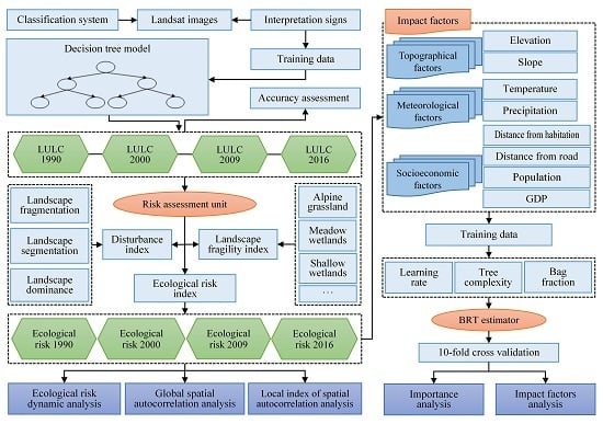
2. Materials and Methods

2.1. Study Area

The Zoige Plateau is located in the northeastern Qinghai–Tibet Plateau. The plateau hosts the largest alpine marsh wetland in the world, and the wetland and alpine meadow areas in this region form a unique alpine wetland ecosystem [32]. The Zoige Plateau is regarded as a sensitive and early warning region for global climate change because it is situated at specific elevations and geographic location [33,34]. The study area consists of parts of Maqu and Luqu Counties in Gansu Province and Ruoergai, Hongyuan, and Aba Counties in Sichuan Province, with a total area of 22,080 km2. It is bounded by the geographic coordinates 101°36′–103°30′E, 32°20′–34°00′N. The elevation of the study area ranges from 3400 m to 3900 m, with an average of 3500 m. There are broad valleys, widely distributed terraces, and a large number of marshes. This area has a semi-humid continental monsoon climate in the sub-frigid zone of the plateau. The region exhibits obvious alpine characteristics, such as long winters and extremely short summers, a cold and dry climate, a long sunshine duration and a short frost-free period. The annual average temperature range is 0–2 °C and the annual precipitation ranges from 600 to 800 mm [35]. There are rich and diverse types of vegetation, which are dominated by alpine grassland, swampland, shrubland, and forest [23]. The soil types include bog soil, peat soil, meadow soil and dark felt-like soil [22]. The river systems within the study area include the main stream and tributaries of the Yellow River, with the Heihe River and Baihe River running from south to north [36]. The wetlands on the Zoige Plateau store 840 million m3 of water. Hence, this area is an important water conservation and supply zone for the upper reaches of the Yellow and Yangtze Rivers [37]. As one of the highest quality natural pastures in Asia, these meadows provide extensive grazing areas, with resident populations of ethnic Gansu and Sichuan minorities (Figure 1).

2.2. Data Sources

2.2.1. Field Data

We conducted field sampling between July and August 2017 and 2018 to establish interpretation signs. We used handheld GPS devices to locate the sampling site and then recorded the land cover type in easily accessible places. In remote and poorly accessible areas, we used a lightweight unmanned aerial vehicle (UAV) to conduct surveys involving the collection of images, GPS information and land cover types. We acquired 224 GPS points and 70 UAV field samples in total. Based on the field GPS information and UAV images, the main types of indicators were established through comparison with the Landsat images (Table S1).

2.2.2. Remote Sensing Data

A total of 16 scenes of Landsat TM/ETM/OLI images (path and row: 131/036, 131/037, 131/038, and 130/037) were downloaded from the United States Geological Survey (USGS) (https://earthexplorer.usgs.gov/). The high-quality images were at 30 m resolution and were obtained between July and August under cloud cover conditions of less than 5%. The data preprocessing mainly included radiometric calibration, atmospheric correction, mosaicking and clipping. The tasseled cap transformation of images from 1990 to 2016 was performed to obtain the brightness component (brightness index, BI) by ENVI5.3 software [38]. The normalized difference vegetation index (NDVI) and the normalized difference water index (NDWI) of the four stages were calculated with ArcGIS10.2 software [39,40]. Gaofen-1 (GF-1) is a high-resolution optical satellite for remote sensing launched by China in 2013 [41]. The images were downloaded from the China Centre for Resources Satellite Data and Application (http://www.cresda.com/CN/). The GF-1 images have a spatial resolution of greater than 8 m and were taken between July and August 2016. GF-1 and Google Earth images were used to verify the precision of the classification results due to limited field measurement data. The topographic data include elevation and slope. The digital elevation model (DEM) is the global digital elevation dataset ASTER GDEM V2, which has a resolution of 30 m (http://srtm.csi.cgiar.org/). The raster surface was adopted to calculate the slope data with a resolution of 30 m in ArcGIS10.2 software. The meteorological data include annual average temperature and annual precipitation for 1990, 2000, 2009 and 2016, with a spatial resolution of 1 km. The socioeconomic data include population and GDP (gross domestic product) in these four stages, with a spatial resolution of 1 km. The spatialization methods and the sources of data can be found at http://www.resdc.cn/.

2.3. Methods

The overall method used for ERA and impact factors analysis is shown in Figure 2. Firstly, the decision tree algorithm with visual interpretation methods and Landsat images was used to classify the LULC types on the study area. Secondly, the study area was divided into many (i.e., 989) risk regions. The ERA model was established to combine the landscape disturbance index and landscape fragmentation index. Finally, the BRT model was adopted to analyze the driving factors of ERA results from the perspectives of topography, climate and socioeconomic factors.

2.3.1. Classification and Accuracy Assessment Methods

According to the classification system in reference [42] and our requirements, eight LULC types were classified for the study area: alpine grassland, meadow wetland, shallow marshes, deep marshes, river and lake, aeolian sediment, construction land and gravel land. Based on consideration of classification accuracy and efficiency, visual interpretation and decision tree classification methods were used to classify the LULC types in 1990, 2000, 2009 and 2016 [43,44]. The visual interpretation method was adopted to extract information about the marsh wetlands and construction land, and then the decision trees were established by utilizing four classification variables (i.e., NDWI, NDVI, DEM, BI) based on 294 field investigation samples and 246 GF-1/Google Earth images points (Table 1, Method S1). When the ground types of field samples collected in 2017–2018 were the same as the Landsat image interpretation types in the study period (1990, 2000, 2009 and 2016), these samples were taken as truth points in the study period. In order to ensure the same quantity, if the LULC types of the field samples changed, then the GF-1 images were used to determine the LULC type in 2016, and the Google Earth images were used to determine the LULC types in 1990, 2000 and 2009. In addition, to assess the accuracy of classification results, another 1147 samples were used to validate the accuracy of the predictions (Table 1). These reference samples from GF-1 images and Google Earth historical images were used to verify the classification results. We established the standard confusion matrix to evaluate the classification accuracy of images in 1990, 2000, 2009 and 2016. The total number of samples correctly classified was divided by the total number of validation samples to calculate the overall accuracy. We also calculated user accuracy (UA), producer accuracy (PA) and Kappa coefficient, respectively [45,46].

2.3.2. LULC Dynamic Degree Model

The dynamic degrees of LULC can directly reflect the range and speed of changes in LULC types [47]. In this study, the comprehensive LULC dynamic degrees model proposed by Gao et al. was used to calculate and analyze the LULC dynamic degrees in the study area from 1990 to 2016 [48]. The formula is as follows:
S   =   Δ S i j   +   Δ S j i S i   ×   1 t   ×   100 %
where S is the dynamic degrees of the LULC type; Si is the total area of an LULC type at the start of monitoring; ΔSi−j is the lost area of an LULC type in the study period; ΔSj−i is the added area of an LULC type in the study period; and t is the time in years.

2.3.3. Construction of the Land Use/Cover ERA Model

To use the empirical relation between the landscape pattern and the ecological environment based on landscape ecology theories and spatial statistical analysis, the disturbance index (EI) and landscape fragility index (FI) were constructed to express the ecological risk quantitatively. EI can measure the degree of disturbance by natural and human factors. This index is used to determine the resistance of the landscape pattern to external disturbance (Method S2). FI refers to the resistance of different landscape types to external disturbance. The lower the value, the higher the resistance of the landscapes in the region to external disturbance and the more stable the ecosystem [49]. FI was obtained through expert consultation method and normalization [50]. Eight landscape types were assigned values according to their ability to resist external influences on the basis of the actual condition of landscape classification in the study area. The FI values after normalization (in decreasing order) were as follows: meadow wetlands = 0.2220, shallow marshes = 0.1944, deep marshes = 0.1667, aeolian sediments = 0.1389, alpine grassland = 0.1110, river and lake = 0.0833, construction land = 0.0556 and gravel land = 0.0278.
The ecological risk index (ERI) was constructed based on the aforementioned landscape disturbance index and the fragmentation index. The higher the index value, the higher the ecological risk of the unit being assessed [51]. The ERI can be expressed as follows:
E R I   = i = 1 n A i A n ( E I i   ×   F I i )
where n is the number of landscape types in the sample area; Ai is the area of landscape i in the sample area; An is the total area of the samples; EIi is the disturbance index of landscape i; and FIi is the fragility index of landscape i.
The study area was separated into 989 ecological risk sampling subareas with a grid of 5 km × 5 km according to equal distance sampling methods, where each subarea was an ERA unit. The comprehensive ecological risk values of different ERA units were calculated individually to obtain the ecological risk level for the center point of the unit, which was the sample for the spatial interpolation analysis within the ERA [52]. An ordinary Kriging interpolation in the geostatistical module of ArcGIS10.2 was used to obtain the spatial distribution for the landscape ecological risk of the Zoige Plateau [24,53]. Combined with the actual condition and the ERI values of the area in the four stages as well as the classification method of Lv et al. and Zhang et al., the ERI was classified into five ecological risk levels [23,27], namely, the lowest-level risk (ERI ≤ 0.050), lower-level risk (0.050 < ERI ≤ 0.060), moderate-level risk (0.060 < ERI ≤ 0.070), higher-level risk (0.070 < ERI ≤ 0.085) and highest-level risk (ERI > 0.085).

2.3.4. Spatial Autocorrelation Analysis Methods

The spatial autocorrelation analysis describes whether a significant correlation is present between the attribute value of a certain element and those of its neighboring elements. This value reflects the spatial correlation characteristics of the spatial reference unit and neighboring units in terms of their characteristic attribute value. Moran’s I is a commonly applied statistical index used to measure global spatial autocorrelation. In this study, Moran’s I was used to measure the global spatial autocorrelation of ecological risk [54,55]. The calculation formula is given below [27]:
G l o b a l   M o r a n s   I   =   i = 1 n j = 1 m w i j ( x i     x ¯ )   ( x j     x ¯   ) s 2 i = 1 n j   = 1 m W i j
S 2   =   1 n   i = 1 n   ( x i     x ) 2
x ¯   =   1 n i = 1 n x i
where xi is the observation value of area i, xj is the observation value of area j; n is the number of grids; Wij is the binary weight matrix of the adjacent space used to represent the adjacency relation of spatial objects; S2 is the mean square deviation. i = 1, 2, …, n; j = 1, 2, …, m; when area i is adjacent to area j, Wij = 1, otherwise, Wij = 0.
The local index of spatial autocorrelation (LISA) is a series of indexes obtained through the direct decomposition of global spatial autocorrelation indexes, and it can be used to determine the spatial difference between region i and its surrounding regions. Moran’s I scatter plot is used to directly reflect the spatial autocorrelation in Geoda1.6.0 software. Under a certain significance level, the LISA cluster gram is obtained in combination with Moran’s I scatter plot. A LISA cluster gram can reflect the spatial heterogeneity and identify the hotspots and cold spots of land use ecological risk in the local space [7,56].

2.3.5. Boosted Regression Tree (BRT) Model

BRT model is a machine learning method based on the classification and regression tree (CART) method [57]. BRT is composed of two algorithms, namely, the regression tree (RT) algorithm and the boosting algorithm. The RT algorithm is used to segment a dataset into many groups of data that are easily modeled by recursion, and then modeling is performed by linear regression. The boosting algorithm is used to enhance the precision of a weak classification algorithm by constructing a series of forecasting functions and then combining them into a single forecasting function in a certain way [57]. The BRT model improves the stability and accuracy of the calculation results. The relative importance of each predictor variable can be obtained when the BRT model was built, therefore, the higher the relative importance, the stronger the effect of the variable on the response. Moreover, the partial dependence graph on the BRT model shows the influence of a predictor on the response after accounting for the average effects of the remaining variables.
In this study, the ERI values of the four stages from 1990 to 2016 were used as dependent variables, the elevation, slope, annual average temperature, annual precipitation, distance from residential areas, distance from road, population and GDP were viewed as independent variables. The eight driving factors are shown in Figure 3. The elevation, slope, distance from residential areas are static variables, the annual average temperature, annual precipitation, population and GDP are dynamic variables.
The value of ecological risk was selected as the response variable. None of the eight predictor variables were highly correlated (R2 < 0.456, Table 2). The “gbm” package programmed by Elith et al. was run in R studio (version 1.2.5) for the BRT analysis [57]. The BRT model with a Gaussian distribution was adopted to investigate the influence of various factors on the ecological risk.
Three parameters are needed in the BRT model, including learning rate (lr), tree complexity (tc) and bag fraction. The learning rate decreases their contributions when each tree is added to the growth model. The tree complexity determines the maximum order of interaction in each tree. When the lr decreases, the ntree increases, which increases the computational cost, but a smaller lr (and larger ntree) tends to get better results [58]. The bag fraction specifies the proportion of training sets used for modeling in each step [30]. Generally, it was reasonable to set the bag fraction to 0.2 [58]. In order to determine the optimal combination of the lr, tc and the number of trees (ntree), models were fitted with lr = 0.05, 0.01, 0.005, 0.001 and tc = 1, 5, 10. Ten-fold cross-validation (CV) was used to verify the accuracy. Figure 4 shows the relationship between the ntree and the prediction deviation under the three tc and four lr values in the model. In general, ntree is optimal when prediction deviation reaches the minimum. The BRT model requires high stability because it is susceptible to overfitting [58], therefore, we set lr = 0.01, tc = 5 and ntree = 10,000 as the optimal scheme according to the accuracy evaluation results (Table 3). In this case, the correlation is relatively high (0.88), while the difference between training data correlation and CV correlation is relatively low (0.06).

3. Results

3.1. Spatio-temporal Patterns in LUCC

3.1.1. Classification Results and Accuracy

Figure 5 shows the spatial distribution map of LULC types on the Zoige Plateau for the four stages from 1990 to 2016. Alpine grassland, shallow marshes and meadow wetlands are the dominant LULC types on the Zoige Plateau, accounting for 71.77%, 12.36% and 9.48% of the total area, respectively.
The accuracy of the classification results was evaluated by calculating the overall accuracy and Kappa coefficients combined with GPS verification points, GF-1 and Google Earth images. The classification results for the four image stages in 1990, 2000, 2009 and 2016 have overall accuracy levels of 88.83%, 87.45%, 89.10% and 90.50%, respectively, with a total average of 89% and they have Kappa coefficients of up to 0.85 (Table 4). These results meet the requirements of this study.

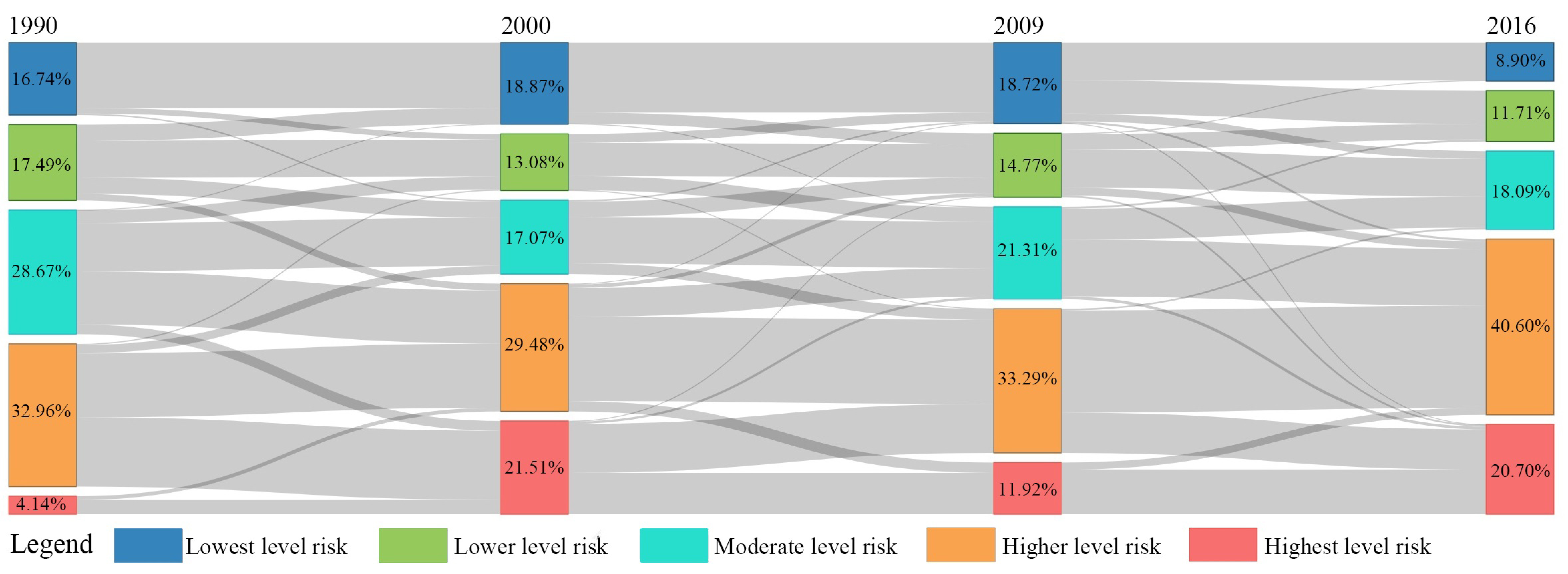
3.1.2. LULC Dynamics Change in 1990–2016

Table 5 shows the area changes and dynamic degrees for the LULC in the study area from 1990 to 2016. Based on the comprehensive dynamic degree research method of Xu et al., landscape change can be divided into four types: extremely slow change (0% to 3%), slow change (3% to 12%), rapid change (12% to 20%) and extremely rapid change (20% to 24%) [59]. Table 5 shows that the LULC changes in the study area from 1990 to 2000 corresponded mainly to the extremely slow type and the slow type. In particular, the meadow wetlands changed the most remarkably, with a comprehensive dynamic degree of up to 11.77%. The dynamic degrees of deep marshes, aeolian sediments and construction land were also relatively high compared with those of other LULC types, all exceeding 8%. The dynamic degree of alpine grassland was the lowest (1.34%), corresponding to the extremely slow change type. From 2000 to 2009, some LULC types exhibited rapid changes and extremely rapid changes. In particular, the change in construction land was the most dramatic, with a dynamic degree exceeding 20%. The LULC dynamic degrees of deep marshes (16.85%) and aeolian sediments (16.81%) were also significant, both exceeding 16%. Compared to those before 2009, the comprehensive dynamic degrees of various ground objects in the study area tended to increase from 2009 to 2016. In particular, the dynamic degree of deep marshes reached 21.67% and was extremely rapid. The aeolian sediments (18.74%), gravel land (16.63%) and construction land (15.10%) also changed significantly and corresponded to the rapid change type. The alpine grassland was still in an extremely slow change state, with a dynamic degree of only 1.47%.

3.2. Analysis of Landscape Ecological Risk

3.2.1. Spatio-temporal Characteristics of Landscape Ecological Risk

In general, the ecological risk on the Zoige Plateau has increased (Figure 6). In particular, the areas with the higher- and moderate-level risk are large. The Zoige Plateau shows significant spatial differences in ecological risk, exhibiting a distribution pattern with higher risk levels in the east and center and lower risk levels in the west and surroundings.
Figure 7 shows the dynamic changes and transfer direction of various types of ecological risk on the Zoige Plateau. From 1990 to 2000, the lower-level risk, moderate-level risk and high-level risk regions in the study area underwent notable changes. In particular, the proportion of lower-level risk areas decreased from 17.49% to 13.08% and primarily transformed into low- and moderate-level risk areas. The proportion of moderate-level risk areas decreased from 28.67% to 17.07% and these areas primarily transformed into higher-level risk areas. The proportion of highest-level risk areas increased from 4.14% to 21.51%, exhibiting the largest change in area among the risk levels, through the transformation of primarily higher- and moderate-level risk areas. From 2000 to 2009, the moderate- and highest-level risk areas changed to a relatively remarkable extent, and in particular, the highest-level risk area changed the most. The proportion of moderate-level risk areas increased from 17.07 to 21.31% through the transformation of higher- and lower-level risks. The proportion of the highest-level risk areas decreased from 21.51 to 11.92% and primarily transformed into higher-level risk areas. From 2009 to 2016, all types levels of ecological risk showed notable changes, and the lowest-, higher- and highest-level risk areas changed the most. The proportion of the lowest-level risk areas decreased from 18.72% in 2009 to 8.9% in 2016 and transformed primarily into lower-level risk areas. The proportion of the higher-level risk area increased from 33.29 to 40.60% through transformation of mainly moderate-level risk areas. The proportion of the highest-level risk area increased from 11.92 to 20.70% through the transformation of mainly higher-level risk areas.

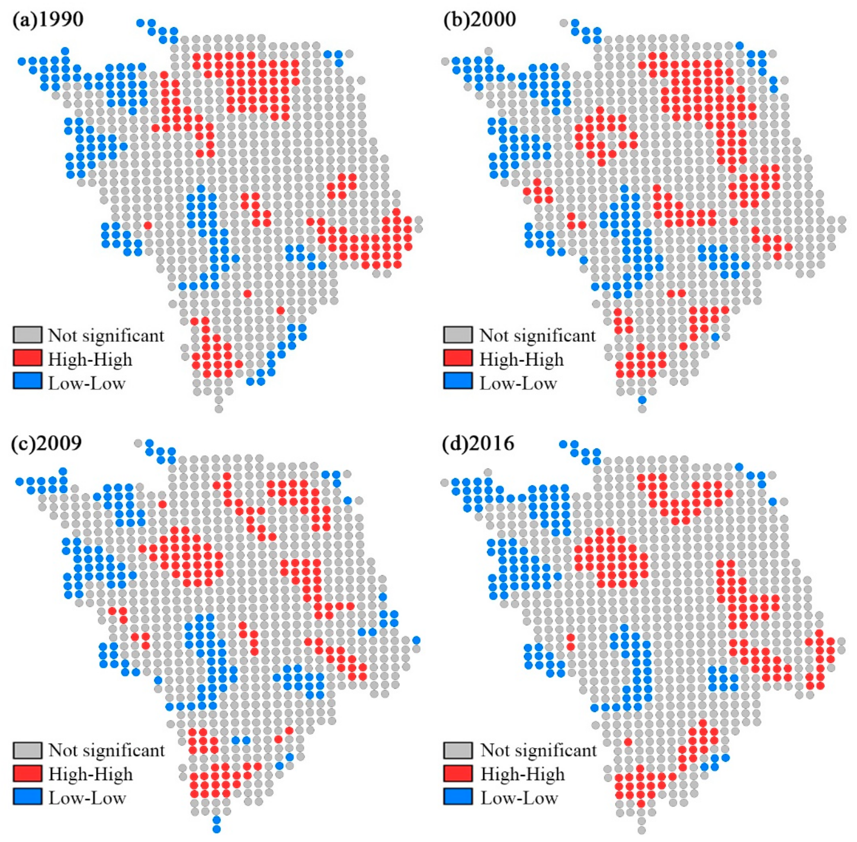
3.2.2. Global Spatial Autocorrelation of Ecological Risk Index (ERI)

Using the spatial distribution data on ecological risk from the Zoige Plateau from 1990 to 2016, Moran’s I scatter plots (Figure 8) were obtained. The global Moran’s I values of ecological risk for the Zoige Plateau were high, reaching 0.7803, 0.7402, 0.7410 and 0.7693 in 1990, 2000, 2009 and 2016, respectively. These results indicate that the ecological risk of the study area shows a clustering effect in space and a strong positive correlation. That is, the ecological risks in the regions around areas of relatively high ecological risk are also relatively high, and the ecological risks in the regions around areas of relatively low ecological risk are also relatively low.

3.2.3. Local Spatial Autocorrelation of ERI

Figure 9 shows that only high–high (HH) and low–low (LL) region autocorrelations are present in the study area. The HH regions are primarily located in the northeastern, central and southernmost parts of the Zoige Plateau, where the marsh wetlands (deep marshes, shallow marshes and meadow wetlands) and aeolian sediments are widely distributed. These types of landscapes are the most fragile and have high ERI values. The LL regions are primarily distributed along the northwestern and southwestern ends of the study area, and the primary LULC types are alpine grassland and gravel land, these landscape types are relatively stable, and thus, the ERI values are relatively low.

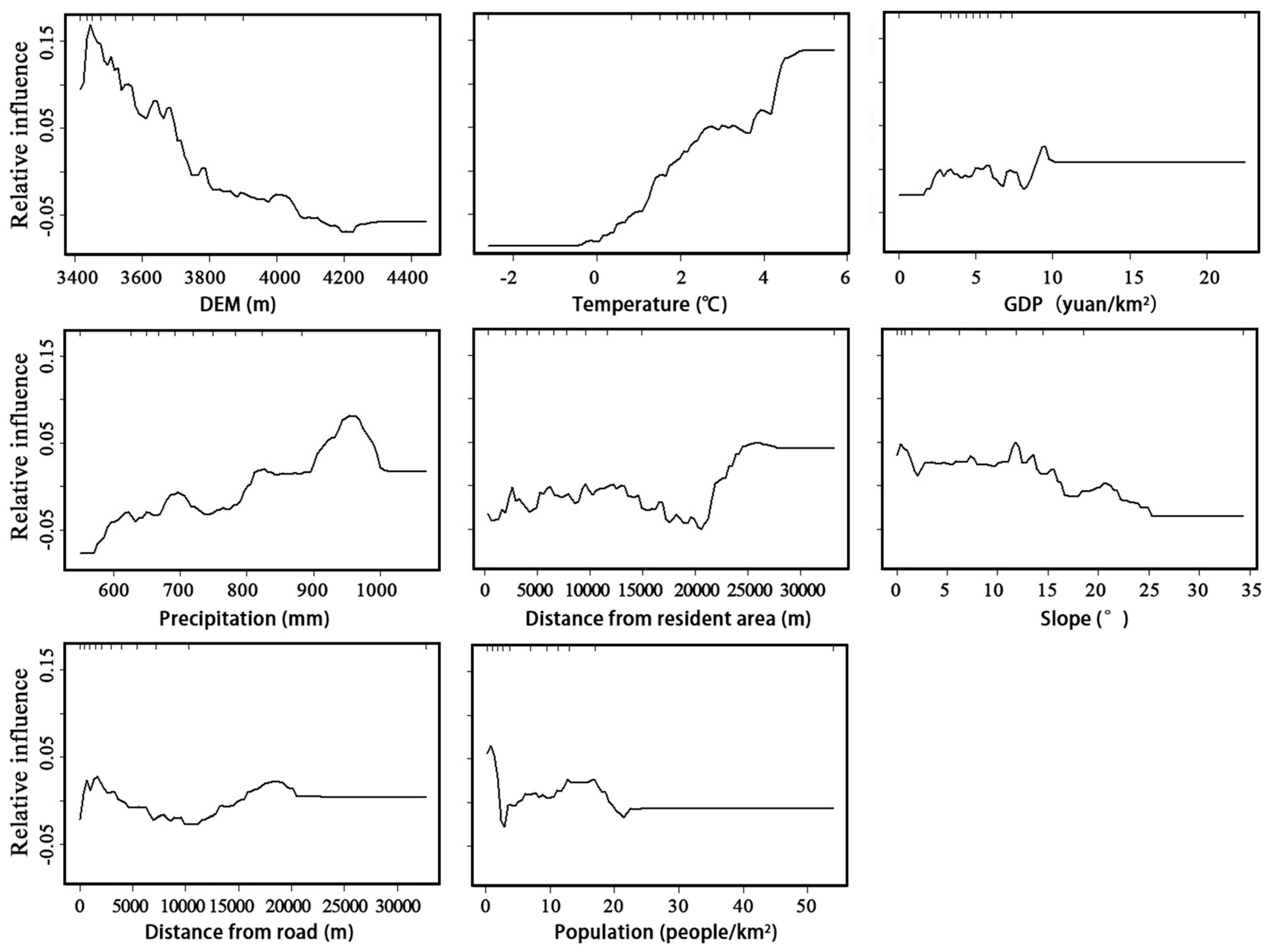
3.3. Analysis of the Impact Factors for ERI

The relative importance of various factors to the ERI of the Zoige Plateau was analyzed using the BRT method (Figure 10). The elevation is the factor that impacts the ERI the most, with a relative importance of 23.4%. The other driving factors in decreasing order of relative importance, are the average temperature (16.2%), GDP (13.0%), annual precipitation (12.1%), distance from residential areas (9.9%), slope (9.0%), distance from roads (8.8%) and population (7.6%).
Figure 11 shows the variation curves for the relative influences of various factors, displaying the changes in factor values and their influences on the ERI. The relative effects of elevation indicate that when the elevation is less than 3740 m, the influence on the ERI is positive. In particular, the influence on the ERI increases with increasing elevation when the elevation is between 3400 and 3460 m, and the influence on the ERI decreases with increasing elevation when the elevation is between 3460 and 3740 m. When the elevation is greater than 3740 m, the influence on the ERI is negative and gradually decreases with increasing elevation. When the temperature is less than 1.7 °C, the influence on the ERI is negative, and this impact decreases with increasing temperature; when the temperature is higher than 1.7 °C, the influence on the ERI is positive, and it increases with increasing temperature. When the GDP is less than 8.5 yuan/km2, the influence of the GDP on the ERI is negative, and in particular, the relative effect is high when the GDP is less than 2.5 yuan/km2. When the GDP is greater than 8.5 yuan/km2, the influence on the ERI displays a positive correlation. When the precipitation is less than 800 mm, the influence on the ERI shows a negative correlation, and the higher the precipitation, the weaker the influence. When precipitation exceeds 800 mm, the influence on the ERI displays a positive correlation. The influence of the distance from residential areas on the ERI first has a negative correlation and then a positive correlation, with a threshold value of 21.9 km. As the slope increases, the value of the ERI first increases and then decreases, with a threshold value of 16°. The influence of the distance from the road on the ERI is primarily within a range of approximately 20 km, and as the distance increases, the influence on the ERI successively shows negative, positive, negative and positive correlations. The relative effect of the population is somewhat irregular, over a range of 4 to 20 people/km2, and the influence on the ERI tends to increase gradually with the increasing population.

4. Discussion

4.1. Mechanisms of Influence on the Ecological Risk

The BRT analysis results of this study indicate that topography, climate and human activities have certain influences on the ecological risk in the study area. In terms of topography, the Zoige Plateau is a hilly plateau with a high elevation [61]. The influence on the ERI is highest when the elevation is within a range of 3400 to 3500 m, primarily because this region is most suitable for human settlements, and the intense human activities in this zone have led to the greatest disturbance.
As the elevation increases, human activities gradually decrease, and the influence on the ERI also decreases accordingly. Because of the challenges posed by the environmental conditions to human activities, few people have settled in this region, and the ERI decreases to the lowest value with decreasing human activity when the elevation exceeds 3800 m. In addition, slope is one of the factors influencing the ERI: the ERI is high when the slope is low, and the ERI is low when the slope is high. The topography of the Zoige Plateau consists primarily of wide valleys and gentle hills. Most of the marsh wetlands are at the bottoms of wide valleys with slopes of <10°; as the slope increases, degradation of the marsh wetlands increases significantly [62], imposing unfavorable influences on the stability of the overall ecosystem and increasing the ecological risk. In addition, human activities are limited to a great extent in steeply sloping regions, and thus, they retain their stable state.
In terms of climate, temperature and precipitation are the primary factors influencing the ERI. The higher the temperature and the lower the precipitation in a region, the relatively higher the ecological risk. According to Figure 12a,b, from 1990 to 2016, the temperature in the study area showed a notable increase, the precipitation basically remained the same, the evaporation increased significantly. With its location east of the Qinghai–Tibet Plateau, the Zoige Plateau is a typical fragile alpine ecological zone and is very sensitive to climate change [63]. In the context of global climate change, the variation in the warming and drying of the Zoige Plateau has caused a decrease in the surface runoff, the drying of marshes, shrinkage of lakes and the desertification of grasslands in this area, resulting in the deterioration of its ecological stability [33,64,65].
Human activities have a significant influence on the ERI. In terms of the GDP, the ecological risk is high when the GDP exceeds 8.5 yuan/km2. Figure 12c shows that the GDP of the study area significantly increased from 1995 to 2015. Due to the specific geographical location and climatic conditions, most regions in this area are not suitable for planting. Animal husbandry is the most important industry in this area, and large animals, such as yaks and Tibetan sheep, and their byproducts are the primary source of income for local farmers. With the rapid economic development and improvement of human living standards in this area, the demand for livestock products has increased and in response, the number of livestock has also increased (Figure 12d), leading to serious overgrazing of the grasslands [66]. The human population has an influence on the ecological risk to a certain extent. Figure 12c shows that the population in each county in the study area has increased gradually over the past 21 years. An increase in the population is also accompanied by an increase in the demand for resources, bringing about enormous pressure on the local area [67]. In the 1970s, to alleviate the population pressure, large-scale trench draining was performed to expand the pasture to meet the grazing demands. The drainage of the trenches deteriorated the water-holding capacity of the wetlands, which is difficult to recover, accelerating the dewatering and shrinkage of marshes and posing a serious threat to the safety and stability of the local ecology [68]. Urban and construction land as a whole did not adversely influence the ecological risk in the study area. Despite the most intense human activities being located in these places, these factors can be effectively planned and managed to maintain stability.

4.2. Innovative Strategies in the Present Study

The method used in this study evaluates the ecological risk of various land cover types in the whole alpine wetland ecosystem on the scale of spatial pixels. Compared with single index assessment, this method comprehensively represents the impact of human activities or natural changes on the landscape composition, structure and function of alpine wetland ecosystems. This approach has good applicability to the eastern part of the Qinghai–Tibet Plateau, which is sensitive to global climate change and is greatly affected by human activities. Compared with the multi-index evaluation method used in recent years, this study takes 5 km × 5 km risk regions as the evaluation unit, which is a finer scale than that of the recent assessment results that take the river basin or township as the smallest unit. Additionally, in view of the limitation that the final directivity of recent landscape ERA are not clear, we used the BRT model and statistical data to quantitatively analyze the driving factors of ecological risk at the pixel scale. Our research provides more refined support for defining the protection objectives and ecological management in the region (i.e., alpine wetland ecosystem).

4.3. The Improvement of Classification and ERA in Future Study

Considering the accuracy and speed of classification, a decision tree with visual interpretation was used to classify the study area. The OA of classification in the four periods can reach 88% on average, and the Kappa coefficient was more than 0.85. The UA and PA of alpine grassland, marsh wetlands and construction land were relatively higher, while those of aeolian sediments were lower. In general, the classification results meet the needs of the present research. The decision tree algorithm is a commonly used automatic machine classification method because of its strong operability, high model interpretation and effectiveness for wetland remote sensing image classification [43]. With the development of computer technology and machine learning algorithms, support vector machine (SVM) and random forest (RF) algorithms have been increasingly adopted in wetland classification. Khatami et al. showed that the classification accuracy of RF and SVM is higher than that of the neural network method (ANN) and maximum likelihood method [69]. Previous researchers have used decision tree and SVM for classification and achieved good results in the Zoige region [22,70]. In the future, the RF method may be an effective way to further improve the classification accuracy of alpine wetland regions. In addition, with the continuous improvement of earth observation systems in various countries, remote sensing data such as Sentinel and GF images have increasing spatial resolution, which has benefits for the more accurate identification of aeolian sediments and addresses the confusion that can arise in the classification of aeolian sediments, meadow grassland and gravel land.
ERA based on landscape patterns is an effective method for performing regional ecological environment assessments of study areas. This method can, not only combine the horizontal interaction of land use systems with the longitudinal interaction of ecosystems, but can also effectively explore their distribution characteristics, local heterogeneity and homogeneity. However, there are still shortcomings. The dominant factors in landscape ecological risk for different study areas vary, and the risk classification setting is still subjective to some extent. Consequently, the classification results can vary. In addition, valuable future studies can include simulating the future LUCC of the study area, combining these changes with ecosystem services and improving and integrating the framework for landscape ERA.

5. Conclusions

Combined with the manual interpretation and machine classification algorithm, and considering both efficiency and precision, the primary ground types of the Zoige Plateau were successfully classified, providing dynamic monitoring of the alpine wetland and alpine grassland resources in the local area from 1990 to 2016. In addition, we performed a spatial analysis on the occurrence of potential ecological risk in the study area, and we determined the factors that influence the ecological stability of the area, providing a basis for local land use management and ecological protection. The primary conclusions are as follows:
(1)
Alpine grassland, alpine wetlands and shallow marshes are the main LULC types on the Zoige Plateau. From 1990 to 2016, the areas of alpine grassland and meadow wetlands showed a gradual increasing trend and the shallow marsh area continuously decreased. From 1990 to 2016, the LULC of the study area experienced remarkable changes, in particular, the changes in deep marshes, aeolian sediments and construction land were the most intense, while the change in alpine grassland was slow.
(2)
From 1990 to 2016, the ecological risk on the Zoige Plateau increased, in particular, regions with higher and moderate ecological risks covered large areas. The ecological risk of the study area showed remarkable spatio-temporal variations, significant spatial correlation and a high degree of spatial clustering.
(3)
The topography, climate and human activities have certain influences on the stability of the alpine wetland ecosystem of the Zoige Plateau. The elevation has the largest influence on the ecological risk of the area, primarily because human activities are the most intense in low-elevation parts of the plateau, disturbing the ecosystems to the greatest extent and causing high ecological risk. Furthermore, warming and drying climate conditions caused decreased surface runoff, the drying of marshes, shrinkage of lakes and the desertification of grasslands, resulting in the deterioration of ecological stability. Economic development has led to an increase in the demand for livestock products, and the resulting increase in the number of livestock has caused overgrazing of pastures and has adversely affected the ecosystem.

Supplementary Materials

The following are available online at https://www.mdpi.com/2072-4292/12/3/368/s1, Table S1: Unmanned Aerial Vehicle (UAV) images and their interpretation signs in study area, Figure S1: Classification rules for various land use/cover types.

Author Contributions

All authors contributed significantly to this article. To be specific, M.H., J.G. (Jing Ge) designed this study and analyzed the data. J.G. (Jinlong Gao), B.M., Y.L., J.Y., and J.L. were responsible for the field investigation, analysis, and paper writing. T.L., Q.F. conceived the idea and contributed to the revision of manuscript. All authors have read and agreed to the published version of the manuscript.

Funding

This research was funded by the National Key Research and Development Program of China Project (2017YFC0504801), the National Natural Science Foundation of China (31672484, 31702175, 41801191 and 41805086), the Program for Changjiang Scholars and Innovative Research Team in University (IRT_17R50), the Earmarked Fund for China Agriculture Research System and the 111 Project (B12002).

Acknowledgments

We acknowledged reviewers and academic editors for their positive and constructive comments and suggestions. We are grateful to the assistance editor and English editor process our manuscript efficient.

Conflicts of Interest

All co-authors declare that there is no conflict of interests.

References

  1. Liu, G.L.; Zhang, L.C.; Zhang, Q.; Musyimi, Z.; Jiang, Q.H. Spatio–temporal dynamics of wetland landscape patterns based on remote sensing in Yellow River Delta, China. Wetlands 2014, 34, 787–801. [Google Scholar] [CrossRef]
  2. Xia, H.M.; Zhao, W.; Li, A.N.; Bian, J.H.; Zhang, Z.J. Subpixel inundation mapping using landsat-8 OLI and UAV data for a wetland region on the Zoige Plateau, China. Remote Sens. 2017, 9, 31. [Google Scholar] [CrossRef] [Green Version]
  3. Li, Y.F.; Liu, H.Y. Advance in wetland classification and wetland landscape classification researches. Wetl. Sci. 2014, 1, 102–108. [Google Scholar]
  4. Liu, Z.W.; Li, S.N.; Wei, W.; Song, X.J. Research progress on alpine wetland changes and driving forces in Qinghai-Tibet Plateau during the last three decades. Chin. J. Ecol. 2019, 38, 856–862. [Google Scholar]
  5. Zhao, Z.L.; Zhang, Y.L.; Liu, L.S.; Zhang, H.F. Recent changes in wetlands on the Tibetan Plateau: A review. J. Geogr. Sci. 2015, 25, 879–896. [Google Scholar] [CrossRef] [Green Version]
  6. Cadavid Restrepo, A.M.; Yang, Y.R.; Hamm, N.A.S.; Gray, D.J.; Barnes, T.S.; Williams, G.M.; Soares Magalhaes, R.J.; McManus, D.P.; Guo, D.H.; Clements, A.C.A. Land cover change during a period of extensive landscape restoration in Ningxia Hui Autonomous Region, China. Sci. Total Environ. 2017, 598, 669–679. [Google Scholar] [CrossRef]
  7. Xie, H.L.; Wang, P.; Huang, H.S. Ecological risk assessment of land use change in the Poyang Lake eco-economic zone, China. Int. J. Environ. Res. Public Health. 2013, 10, 328–346. [Google Scholar] [CrossRef] [Green Version]
  8. Liu, D.; Chen, H.; Liang, X.Y.; Ma, S.; Wang, J.N. The dynamic changes to ecological risk in the Loess Hilly-gully region and its terrain gradient analysis: A case study of Mizhi County, Shaanxi Province, China. Acta Ecol. Sin. 2018, 38, 8584–8592. [Google Scholar]
  9. Zhao, Z.; Zhang, T. Integration of ecosystem services into ecological risk assessment for implementation in ecosystem based river management: A case study of the Yellow River, China. Hum. Ecol. Risk Assess. 2013, 19, 80–97. [Google Scholar] [CrossRef]
  10. Malekmohammadi, B.; Blouchi, L.R. Ecological risk assessment of wetland ecosystems using multi criteria decision making and geographic information system. Ecol. Indic. 2014, 41, 133–144. [Google Scholar] [CrossRef]
  11. Li, Q.P.; Zhang, Z.D.; Wan, L.W.; Yang, C.X.; Zhang, J.; Chen, Y.E.; Chen, Y. Landscape pattern optimization in Ningjiang River Basin based on landscape ecological risk assessment. Acta Geogr. Sin. 2019, 74, 1420–1437. [Google Scholar]
  12. Cao, Q.W.; Zhang, X.W.; Ma, H.K.; Wu, J.S. Review of landscape ecological risk and an assessment framework based on ecological services: ESRISK. Acta Geogr. Sin. 2018, 73, 843–855. [Google Scholar]
  13. Piggott, J.J.; Townsend, C.R.; Matthaei, C.D. Re-conceptualizing synergism and antagonism among multiple stressors. Ecol. Evol. 2015, 5, 1538–1547. [Google Scholar] [CrossRef] [PubMed]
  14. Ban, S.S.; Graham, N.A.J.; Connolly, S.R. Evidence for multiple stressor interactions and effects on coral reefs. Glob. Chang. Biol. 2014, 20, 681–697. [Google Scholar] [CrossRef]
  15. Jiang, T.T.; Pan, J.F.; Pu, X.M.; Wang, B.; Pan, J.J. Current status of coastal wetlands in China: Degradation, restoration, and future management. Estuar. Coast. Shelf Sci. 2015, 164, 265–275. [Google Scholar] [CrossRef]
  16. Landis, W.G. Twenty years before and hence; Ecological risk assessment at multiple scales with multiple stressors and multiple endpoints. Hum. Ecol. Risk Assess. 2003, 9, 1317–1326. [Google Scholar] [CrossRef]
  17. Tian, P.; Shi, X.L.; Li, J.L.; Wang, L.L.; Liu, R.P. Land use change and ecological risk assessment in Hang Zhou city. Bull. Soil Water Conserv. 2018, 38, 274–281. [Google Scholar]
  18. Liu, X.; Su, W.C.; Wang, Z.; Huang, Y.M.; Deng, J.X. Regional ecological risk assessment of land use in the flooding zone of the Three Gorges Reservoir area based on relative risk model. Acta Sci. Circumstantiae 2012, 32, 248–256. [Google Scholar]
  19. Zhou, Q.G.; Zhang, X.Y.; Wang, Z.L. Land use ecological risk evaluation in Three Gorges Reservoir area based on normal cloud model. Trans. Chin. Soc. Agric. Eng. 2014, 30, 289–297. [Google Scholar]
  20. Guo, K.; Kuai, X.; Chen, Y.; Qi, L.; Zhang, L.; Liu, Y. Risk assessment of land ecology on a regional scale: Application of the relative risk model to the mining city of Deye, China. Hum. Ecol. Risk Assess. Int. J. 2017, 23, 550–574. [Google Scholar] [CrossRef]
  21. Bartolo, R.E.; Van Dam, R.A.; Bayliss, P. Regional ecological risk assessment for Australia’s Tropical Rivers: Application of the relative risk model. Hum. Ecol. Risk Assess. Int. J. 2012, 18, 16–46. [Google Scholar] [CrossRef]
  22. Shen, G.; Yang, X.C.; Jin, Y.X.; Xu, B.; Zhou, Q.B. Remote sensing and evaluation of the wetland ecological degradation process of the Zoige Plateau Wetland in China. Ecol. Indic. 2019, 104, 48–58. [Google Scholar] [CrossRef]
  23. Jiang, W.G.; Lv, J.X.; Wang, C.C.; Chen, Z.; Liu, Y.H. Marsh wetland degradation risk assessment and change analysis: A case study in the Zoige Plateau, China. Ecol. Indic. 2017, 82, 316–326. [Google Scholar] [CrossRef]
  24. Jin, X.; Jin, Y.X.; Mao, X.F. Ecological risk assessment of cities on the Tibetan Plateau based on land use/land cover changes – Case study of Delingha City. Ecol. Indic. 2019, 101, 185–191. [Google Scholar] [CrossRef]
  25. Lv, L.T.; Zhang, J.; Sun, C.Z.; Wang, X.R.; Zheng, D.F. Landscape ecological risk assessment of Xi river Basin based on land-use change. Acta Ecol. Sin. 2018, 38, 5952–5960. [Google Scholar]
  26. Mo, W.B.; Wang, Y.; Zhang, Y.X.; Zhuang, D.F. Impacts of road network expansion on landscape ecological risk in a megacity, China: A case study of Beijing. Sci. Total Environ. 2017, 574, 1000–1011. [Google Scholar] [CrossRef] [Green Version]
  27. Zhang, F.; Yushanjiang, A.; Wang, D.F. Ecological risk assessment due to land use/cover changes (LUCC) in Jinghe County, Xinjiang, China from 1990 to 2014 based on landscape patterns and spatial statistics. Environ. Earth Sci. 2018, 77, 491. [Google Scholar] [CrossRef]
  28. Glenn, D. Boosted trees for ecological modeling and prediction. Ecology 2007, 88, 243–251. [Google Scholar]
  29. Main, A.R.; Michel, N.L.; Headley, J.V.; Peru, K.M.; Morrissey, C.A. Ecological and landscape drivers of neonicotinoid insecticide detections and concentrations in Canada’s prairie wetlands. Environ. Sci. Technol. 2015, 49, 8367–8376. [Google Scholar] [CrossRef]
  30. Zhang, W.J.; Du, Z.C.; Zhang, D.M.; Yu, S.C.; Hao, Y.T. Boosted regression tree model-based assessment of the impacts of meteorological drivers of hand, foot and mouth disease in Guangdong, China. Sci. Total Environ. 2016, 553, 366–371. [Google Scholar] [CrossRef]
  31. Elisa, S.V.; Walter, V.; Morgan, P.; Catherine, L.; José, P.G.; Diamantina, M.G.; Philippe, L.; Alejandro, L.C.; Niko, S.; Marie-Pierre, H.; et al. Malaria risk assessment and mapping using satellite imagery and boosted regression trees in the Peruvian Amazon. Sci. Rep. 2019, 9, 15173. [Google Scholar]
  32. Huo, L.L.; Chen, Z.K.; Zou, Y.C.; Lu, X.G.; Guo, J.W.; Tang, X.G. Effect of Zoige alpine wetland degradation on the density and fractions of soil organic carbon. Ecol. Eng. 2013, 51, 287–295. [Google Scholar] [CrossRef]
  33. Bai, J.H.; Wang, J.J.; Zhao, Q.Q.; Hua, O.; Wei, D. Landscape pattern evolution processes of alpine wetlands and their driving factors in the Zoige Plateau of China. J. Mater. Sci. 2013, 10, 54–67. [Google Scholar] [CrossRef]
  34. Shen, G.; Xu, B.; Jin, Y.X.; Chen, S.; Zhang, W.B.; Guo, J.; Liu, H.; Zhang, Y.J.; Yang, X.C. Advances in studies of wetlands in Zoige Plateau. Geogr. Geo-Inf. Sci. 2016, 32, 76–82. [Google Scholar]
  35. Zhang, Y.; Wang, G.X.; Wang, Y.B. Changes in alpine wetland ecosystems of the Qinghai-Tibetan Plateau from 1967 to 2004. Environ. Monit. Assess. 2011, 180, 189–199. [Google Scholar] [CrossRef] [PubMed] [Green Version]
  36. Dong, Z.B.; Hu, G.Y.; Yan, C.Z.; Wang, W.L.; Lu, J.F. Aeolian desertification and its causes in the Zoige Plateau of China’s Qinghai-Tibetan Plateau. Environ. Earth Sci. 2010, 59, 1731–1740. [Google Scholar] [CrossRef]
  37. Yang, Y.X.; Li, K.; Yang, Y. Evaluation index system of swamp degradation in Zoige Plateau of Sichuan. Chin. J. Appl. Ecol. 2013, 24, 1826–1836. [Google Scholar]
  38. Mukhopadhyay, A.; Ghosh, P.; Chanda, A.; Ghosh, A.; Ghosh, S.; Das, S.; Ghosh, T.; Hazra, S. Threats to coastal communities of Mahanadi delta due to imminent consequences of erosion-present and near future. Sci. Total Environ. 2018, 637–638, 717–729. [Google Scholar] [CrossRef]
  39. Ge, J.; Meng, B.P.; Liang, T.G.; Feng, Q.S.; Gao, J.L. Modeling alpine grassland cover based on MODIS data and support vector machine regression in the headwater region of the Huanghe River, China. Remote Sens. Environ. 2018, 218, 162–173. [Google Scholar] [CrossRef]
  40. Tri, A.; Anoj, S.; Dong, L. Evaluation of water indices for surface water extraction in a Landsat 8 scene of Nepal. Sensors 2018, 18, 2580. [Google Scholar]
  41. Liu, Q.Y.; Yu, T.; Zhang, W.H. Validation of GaoFen-1 Satellite Geometric Products Based on Reference Data. J. Indian Soc. Remote Sens. 2019, 47, 1331–1346. [Google Scholar] [CrossRef]
  42. Yu, K.F.; Lehmkuhl, F.; Falk, D. Quantifying land degradation in the Zoige Basin, NE Tibetan Plateau using satellite remote sensing data. J. Mt. Sci. 2017, 14, 77–93. [Google Scholar] [CrossRef]
  43. Xiao, F.Y.; Gao, G.Y.; Shen, Q.; Wang, X.F.; Ma, Y.; Lü, Y.; Fu, B. Spatio-temporal characteristics and driving forces of landscape structure changes in the middle reach of the Heihe River Basin from 1990 to 2015. Landsc. Ecol. 2019, 34, 755–770. [Google Scholar] [CrossRef]
  44. Zhang, F.; Yushanjiang, A.; Jing, Y.Q. Assessing and predicting changes of the ecosystem service values based on land use/cover change in Ebinur Lake Wetland National Nature Reserve, Xinjiang, China. Sci. Total Environ. 2019, 656, 1133–1144. [Google Scholar] [CrossRef] [PubMed]
  45. Luo, K.S.; Li, B.J.; Juana, P.M. Monitoring Land-Use/Land-Cover Changes at a Provincial Large Scale Using an Object-Oriented Technique and Medium-Resolution Remote-Sensing Images. Remote Sens. 2018, 10, 2012. [Google Scholar] [CrossRef] [Green Version]
  46. Cao, J.J.; Liu, K.; Liu, L.; Zhu, Y.H.; Li, J.; He, Z. Identifying Mangrove Species Using Field Close-Range Snapshot Hyperspectral Imaging and Machine-Learning Techniques. Remote Sens. 2018, 10, 2047. [Google Scholar] [CrossRef] [Green Version]
  47. Lin, Q.Y.; Guo, J.Y.; Yan, J.F.; Wang, H. Land use and landscape pattern changes of Weihai, China based on object-oriented svm classification from landsat MSS/TM/OLI images. Eur. J. Remote Sens. 2018, 51, 1036–1048. [Google Scholar] [CrossRef] [Green Version]
  48. Gao, X.Y.; Cheng, W.M.; Wang, N.; Liu, Q.Y.; Ma, T.; Chen, Y.J.; Zhou, C.H. Spatio-temporal distribution and transformation of cropland in geomorphologic regions of China during 1990–2015. J. Geogr. Sci. 2019, 29, 180–196. [Google Scholar] [CrossRef] [Green Version]
  49. Shi, H.P.; Yu, K.Q.; Feng, Y.J. Ecological risk assessment of rural-urban ecotone based on landscape pattern: A case study in Daiyue District of Tai’an City, Shandong Province of East China. Chin. J. Appl. Ecol. 2013, 24, 705–712. [Google Scholar]
  50. Gao, B.; Li, X.Y.; Li, Z.G.; Chen, W.; He, X.Y.; Qi, S. Assessment of ecological risk of coastal economic developing zone in Jinzhou Bay based on landscape pattern. Acta Ecol. Sin. 2011, 31, 3441–3450. [Google Scholar]
  51. Zhang, X.B.; Shi, P.J.; Luo, J. Landscape ecological risk assessment of the Shiyang river Basin. Commun. Comput. Inf. 2013, 399, 98–106. [Google Scholar]
  52. Lu, C.; Zhao, Y.H.; Liu, J.C.; Han, L.; Ao, Y.; Yin, S. Landscape ecological risk assessment in Qinling Mountain. Geol. J. 2018, 53, 342–351. [Google Scholar]
  53. Hui, S.; Yang, Z.P.; Fang, H.; Shi, T.G.; Dong, L. Assessing landscape ecological risk for a world natural heritage site: A case study of Bayanbulak in China. Pol. J. Environ. Stud. 2015, 24, 269–283. [Google Scholar]
  54. Anselin, L. Local indicators of spatial association. Geogr. Anal. 1995, 27, 93–115. [Google Scholar] [CrossRef]
  55. Liu, S.L.; Hou, X.Y.; Wu, Y.J.; Cheng, F.Y.; Zhang, Y.Q.; Dong, S.K. Research progress on landscape ecological networks. Acta Ecol. Sin. 2017, 37, 3947–3956. [Google Scholar]
  56. Xie, H.L.; Kung, C.C.; Zhao, Y.L. Spatial disparities of regional forest land change based on ESDA and GIS at the county level in Beijing-Tianjin-Hebei area. Front. Earth Sci. 2012, 6, 445–452. [Google Scholar] [CrossRef]
  57. Elith, J.; Leathwick, J.R.; Hastie, T. A working guide to boosted regression trees. J. Anim. Ecol. 2008, 77, 802–813. [Google Scholar] [CrossRef]
  58. Leticia, V.; Lucía, A.; Alejandra, R.H.; Ana, G.; Karina, M.; Eduardo, B.; Gastón, A. Relationship between astringency and phenolic composition of commercial Uruguayan Tannat wines: Application of boosted regression trees. Food Res. Int. 2018, 112, 25–37. [Google Scholar]
  59. Xu, X.L.; Wang, X.J.; Zhu, X.P.; Jia, H.T.; Han, D.L. Landscape pattern changes in alpine wetland of Bayanbulak Swan Lake during 1996–2015. J. Nat. Resour. 2018, 33, 1897–1911. [Google Scholar]
  60. Ghulam, A.; Ghulam, O.; Maimaitijiang, M.; Freeman, K.; Porton, I.; Maimaitiyiming, M. Remote sensing based spatial statistics to document tropical rainforest transition pathways. Remote Sens. 2015, 7, 6257–6279. [Google Scholar] [CrossRef] [Green Version]
  61. Bai, H.J.; Ouyang, H.; Cui, B.S.; Wang, Q.G.; Chen, H. Changes in landscape pattern of alpine wetlands on the Zoige Plateau in the past four decades. Acta Ecol. Sin. 2008, 28, 2245–2252. [Google Scholar]
  62. Chen, Z.K.; Lv, X.G. Comparison between the Marsh Wetland Landscape Patterns in the Zoige Plateau for two periods. Wetl. Sci. 2010, 8, 8–14. [Google Scholar]
  63. Qiu, P.F.; Wu, N.; Luo, P.; Wang, Z.Y.; Li, M.H. Analysis of dynamics and driving factors of wetland landscape in Zoige, eastern Qinghai-Tibetan Plateau. J. Mt. Sci 2009, 6, 42–55. [Google Scholar] [CrossRef] [Green Version]
  64. Guo, J.; Li, G.P. Zoige climate change and its impact on wetland degradation. Plateau Meteorol. 2007, 26, 422–428. [Google Scholar]
  65. Wang, Y.Y.; He, Y.X.; Ju, P.J.; Zhu, Q.A.; Liu, J.L.; Chen, H. Application of analytic hierarchy process in wetland degradation research. Chin. J. Appl. Environ. Biol. 2019, 25, 46–52. [Google Scholar]
  66. Ding, K.P.; Li, G.Q.; Wang, J.; Lv, T.; Kong, X.X. Influence of human activities to the wetland landscape pattern in Zoige Plateau. Yellow River 2016, 38, 58–63. [Google Scholar]
  67. Yao, L.; Zhao, Y.; Gao, S.J.; Sun, J.H. The peatland area change in past 20 years in the Zoige Basin, eastern Tibetan Plateau. Front. Earth Sci. 2011, 5, 271–275. [Google Scholar] [CrossRef]
  68. Zhang, W.J.; Lu, Q.F.; Song, K.C.; Qin, G.H.; Wang, Y.; Li, H.; Li, J.; Liu, G.; Li, H. Remotely sensing the ecological influences of ditches in Zoige Peatland, eastern Tibetan Plateau. Int. J. Remote Sens. 2014, 35, 5186–5197. [Google Scholar] [CrossRef]
  69. Khatami, R.; Mountrakis, G.; Stehman, S.V. A meta-analysis of remote sensing research on supervised pixel-based land-cover image classification processes: General guidelines for practitioners and future research. Remote Sens. Environ. 2016, 177, 89–100. [Google Scholar] [CrossRef] [Green Version]
  70. Hu, G.Y.; Dong, Z.B.; Wei, Z.H.; Lu, J.F. Land use and land cover change monitoring in the Zoige Wetland by remote sensing. Proc. SPIE Int. Soc. Opt. Eng. 2009, 7841. [Google Scholar] [CrossRef]
Figure 1. (a) Location of the Zoige Plateau in China; (b) a digital elevation model (DEM) of the study area; and (c) the natural color composition (RGB = red, green, blue) of the Landsat-OLI image of the study area in 2016.
Remotesensing 12 00368 g001
Figure 2. A flowchart of the ecological risk assessment and its impact factors analysis in the study.
Remotesensing 12 00368 g002
Figure 3. Impact factors (a) elevation; (b) slope; (c) annual average temperature in 2016; (d) annual precipitation in 2016; (e) distance from resident areas; (f) distance from road in 2016; (g) population in 2015; (h) GDP in 2015.
Remotesensing 12 00368 g003
Figure 4. The relationship between the number of trees and predictive deviance for models fitted with three levels of tree complexity and four learning rates, (a) learning rates = 0.05, (b) learning rate = 0.01, (c) learning rate = 0.005, (d) learning rate = 0.001).
Remotesensing 12 00368 g004
Figure 5. Land use/cover in 1990, 2000, 2009 and 2016.
Remotesensing 12 00368 g005
Figure 6. Maps of the ecological risk level in (a) 1990, (b) 2000, (c) 2009 and (d) 2016.
Remotesensing 12 00368 g006
Figure 7. Ecological risk transformation matrix for 1990, 2000, 2009 and 2016.
Remotesensing 12 00368 g007
Figure 8. Moran scatter plots of the ecological risk in the study area (Low-high: LH, high-high: HH, low-low: LL, high-low: HL.). Under a given significance level, when Moran’s I > 0, there is positive spatial autocorrelation, indicating a clustered state of spatial ecological phenomena; when Moran’s I < 0, there is negative spatial autocorrelation, indicating a discrete state of spatial ecological phenomena. When Moran’s I = 0, there is no spatial autocorrelation, indicating a random distribution of spatial ecological phenomena [60].
Remotesensing 12 00368 g008
Figure 9. The local index of spatial autocorrelation (LISA) cluster maps.
Remotesensing 12 00368 g009
Figure 10. Relative importance of various factors for the ERI in the BRT analysis.
Remotesensing 12 00368 g010
Figure 11. Relative influence on the change in the ERI in the study area. When the value of the relative influence is greater than zero, the influence of various factors is positive; when the value of the relative influence is less than zero, the influence of various factors is negative; and when the value of relative influence equals zero, there is no influence.
Remotesensing 12 00368 g011
Figure 12. Interannual variability in (a) temperature and precipitation, (b) evaporation, (c) population and GDP and (d) large livestock.
Remotesensing 12 00368 g012
Table 1. Number of training and validation data for different land use and land cover (LULC) types.
Land Use/Cover TypesTraining DataValidation Data
GPS SamplesUAV SamplesGF-1/Google Earth
Images Samples
GF-1/Google Earth
Images Samples
Alpine grassland1013019460
Meadow wetlands521137205
Shallow marshes6787200
Deep marshes1662870
River and lake1451150
Aeolian sediments1153480
Construction land226250
Gravel land202832
Total224702461147
Table 2. Pearson correlation coefficients for all pairs of impact factors. V0~V8 represent ecological risk index (ERI), elevation, slope, temperature, precipitation, distance from resident area, distance from road, population and GDP, respectively.
V0V1V2V3V4V5V6V7V8
V01
V1−0.3181
V2−0.2220.4561
V30.260−0.378−0.1771
V4−0.0200.3230.1470.0091
V5−0.0260.1500.038−0.0990.0411
V6−0.0590.1020.027−0.1410.0130.0941
V700.0010−0.0200.0050.00701
V800.0070.0080.00100.010−0.0180.0421
Table 3. The correlation between training data and cross-validation (CV) of three levels of tree complexity (tc1, tc5 and tc10) and four learning rates (lr0.05, lr0.01, lr0.005 and lr0.001).
Learning Ratetc1tc5tc10
Training Data CorrelationCV CorrelationTraining Data CorrelationCV CorrelationTraining Data CorrelationCV Correlation
lr0.050.740.700.950.850.970.85
lr0.010.720.690.880.820.930.84
lr0.0050.710.680.850.790.900.82
lr0.0010.670.660.780.750.820.78
Table 4. Accuracy of land use/cover classification results in 1990, 2000, 2009 and 2016. UA, PA and OA represent user accuracy, producer accuracy and overall accuracy, respectively.
Land Use/Cover Types1990200020092016
UA (%)PA (%)UA (%)PA (%)UA (%)PA (%)UA (%)PA (%)
Alpine grassland85.6593.8184.1393.8189.3592.3693.2693.46
Meadow wetlands95.6188.6993.1788.6993.1784.5195.1287.84
Shallow marshes96.0091.4394.0091.4394.0089.1091.5090.59
Deep marshes97.1497.1497.1497.1490.0098.4487.1498.39
River and lake82.0085.4268.0085.1292.0085.1982.0077.36
Aeolian sediments67.5062.7976.2562.0780.0073.5671.2586.36
Construction land92.0090.2092.0090.2088.0097.7888.0093.62
Gravel land85.2967.4482.3566.6744.1288.2482.3573.69
OA (%)88.8387.4589.1090.50
Kappa coefficient0.870.850.870.88
Table 5. LULC dynamics degree of the study area from 1990 to 2016.
Land Use/Cover Types1990–20002000–20092009–2016
Change Area (km2)Dynamic Degree (%)Change Area (km2)Dynamic Degree (%)Change Area (km2)Dynamic Degree (%)
Alpine grassland2005.101.341604.221.10−1675.581.47
Meadow wetlands2262.1211.771862.439.881475.0910.29
Shallow marshes−2114.996.41−897.653.55−1309.747.30
Deep marshes−206.528.58133.3516.85−128.7121.67
River and lake−167.106.27107.787.06168.1911.12
Aeolian sediments−316.488.64−361.616.81437.6618.74
Construction land45.838.54115.2320.90138.4015.10
Gravel land−604.696.08−305.287.92442.0016.63

