Regional Forest Volume Estimation by Expanding LiDAR Samples Using Multi-Sensor Satellite Data

Abstract

Accurate information regarding forest volume plays an important role in estimating afforestation, timber harvesting, and forest ecological services. Traditionally, operations on forest growing stock volume using field measurements are labor-intensive and time-consuming. Recently, remote sensing technology has emerged as a time-cost efficient method for forest inventory. In the present study, we have adopted three procedures, including samples expanding, feature selection, and results generation and evaluation. Extrapolating the samples from Light Detection and Ranging (LiDAR) scanning is the most important step in satisfying the requirement of sample size for nonparametric methods operation and result in accuracy improvement. Besides, mean decrease Gini (MDG) methodology embedded into Random Forest (RF) algorithm served as a selector for feature measure; afterwards, RF and K-Nearest Neighbor (KNN) were adopted in subsequent forest volume prediction. The results show that the retrieval of Forest volume in the entire area was in the range of 50–360 m³/ha, and the results from the two models show a better consistency while using the sample combination extrapolated by the optimal threshold value (2 × 10⁻⁴), leading to the best performances of RF (R² = 0.618, root mean square error, RMSE = 43.641 m³/ha, mean absolute error, MAE = 33.016 m³/ha), followed by KNN (R² = 0.617, RMSE = 43.693 m³/ha, MAE = 32.534 m³/ha). The detailed analysis that is discussed in the present paper clearly shows that expanding image-derived LiDAR samples helps in refining the prediction of regional forest volume while using satellite data and nonparametric models.

1. Introduction

Forests, as one of the essential terrestrial ecosystems, play an indispensable ecological and social service functions [1,2], being one of the important sources for carbon sink [3,4,5]. The growing stock volume is recognized as one of the most important forest attributes for monitoring forest growth, assessing the yield of timber of plantation and natural forest, and estimating forest biomass, especially, for the forest stand timber harvest operations, i.e., rotation, method, and allowable size requiring accurate information on tree size. Thus, forest stock information, which can improve the efficiency of forest management and reduce the cost of time and labor, is in high demand in the industry sector [6]. The regional tree size results used to be roughly quantified while using diameter-at-breast-height (DBH)-based allometry based on forest inventory data, which is undertaken every five years. Currently, the remote sensing technique has emerged as an important tool for forest inventory, providing continuous and up-to-date information on forest volume, which can help in forest resource management and forest growth observations [7,8,9]. Earlier studies involving the use of multi-source satellite techniques for forest volume prediction can be divided into two categories: using only Airborne Light Detection and Ranging (LiDAR) for accurate and convenient acquisition of small-scale forest volume distributions; and adopting wide-range Synthetic Aperture Radar (SAR) or multi-spectral satellite images, or coordinating multi-sensor data to estimate regional-wide forest volume mappings.

LiDAR is capable of directly capturing the three-dimension information on forest structure via actively transmitting laser pulses that interact with forest structure and then receiving the return signals. It has evolved into the preeminent remotely sensed platform to characterize detailed information of forest attributes spatially, since the end of the last century [10,11,12,13,14,15,16,17,18] due to its high precision and flexibility critical for operational forest management, and it has been extensively adopted for artificial or natural forest attributes monitoring on the individual tree-level [19,20,21] and small-scale [22,23,24]. Moreover, forest volume, as one of the structure parameters, was often accurately estimated by LiDAR [25], for example, Clementel et al. [26] have carried out statistical models combined with medium-resolution LiDAR to produce timber volume mapping, and Lo et al. [19] demonstrated tree growth competition index (LCI) derived from LiDAR scanning while using a rasterized canopy height model (multilevel morphological active-contour algorithm) was a key factor for forest volume estimation. Additionally, the relationship between volume and height and the sensitivity of tree volume estimation to LiDAR trajectory error were implemented [9,27].

Even though LiDAR can acquire horizontal and vertical information on forest structure at high spatial resolutions and vertical accuracies, it was mainly applied over small- and moderate- scale forest applications, owing to the cost constraints [28]. Instead, the optical and SAR remote sensing are more applicable to depicting forest structure over a large area. Since the 20th century, air- and space- imaging technologies (Airborne Imaging Spectrometer, i.e., AIS and Landsat thematic mapper, i.e., TM) were introduced into forest inventory [29,30,31]. The multi-spectral images of high quality and availability have been used to predict regional forest volume, prior to the use of other remote sensing technologies [8,32,33]. Sentinel-2 data have emerged as one of the popular data sources for stock volume mapping, due to its higher resolution and the unique red-edge band sensitive to vegetations since the launch of the Sentinel-2A satellite in 2015 [34,35]. Optical remote sensing still has some drawbacks: it is prone to yielding spectral saturation, leading to an underestimation of the forest structure parameters in the dense forest due to its insufficient penetration through the canopy; meanwhile, the impact of the weather could result in the lack of data in cloudy and rainy days. Nevertheless, SAR remote sensing has all-weather, all-time capabilities, and higher sensitivity for forest structure as compared with optical imaging. SAR satellite data, such as ERS, RADARSAT, JRES, PALSAR, and so on, were diffusely adopted to derive forest growing stock volume [36,37,38,39]; additionally, optical and radar data synergy has also been extensively studied in volume extraction, yielding more reliable precision [37,40,41]. To improve the accuracy of forest volume mapping in large areas, e.g., municipal, provincial, and even larger scales, coordinating high-precision LiDAR scanning and other satellite data was proven to be an important approach [42]. Hawrylo et al. [43] separately used multiple linear regression (LM) and random forest (RF) method to predict stock volume in Scots pine Stand while using Sentinel-2 combining with airborne point clouds, and unmanned aerial vehicles (UAV) combined with Sentinel-2 was also studied for stock volume estimation through a hierarchical model-based mode of inference [44]. In addition, Landsat and LiDAR composites [45], as well as combination of more than two-sensor (LiDAR, Landsat, and PALSAR) [40], were used to predict forest volume distribution.

Although all of the earlier studies have provided various solutions to forest volume prediction, they still suffer from some limitations. One of the main limitations was that the LiDAR-only results could not cover a large area, and the image-derived LiDAR points were directly used as the training and testing samples for regional forest volume inference. When the area of the whole study region was much larger than that of the LiDAR scanning extent, the samples from LiDAR will no longer be able to characterize the distribution of the forest volume across the entire region [46,47]. The objectives of the present study are to expand the original image-derived from LiDAR data with more reasonable distribution throughout the study area, which refers to intensifying the plots to increase the number and spatial frequency of the training samples; to find out the optimal threshold value used in sample expanding; and, to estimate the impact of additionally extrapolating LiDAR samples on the accuracy of predicting outcomes while using the approaches of Random Forest (RF) and K-Nearest Neighbor (KNN), and generate a regional forest volume mapping at ~30 m. The detailed analysis shows a better approach to map forest volume combined with multi-source remotely sensed data.

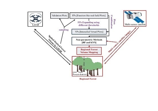
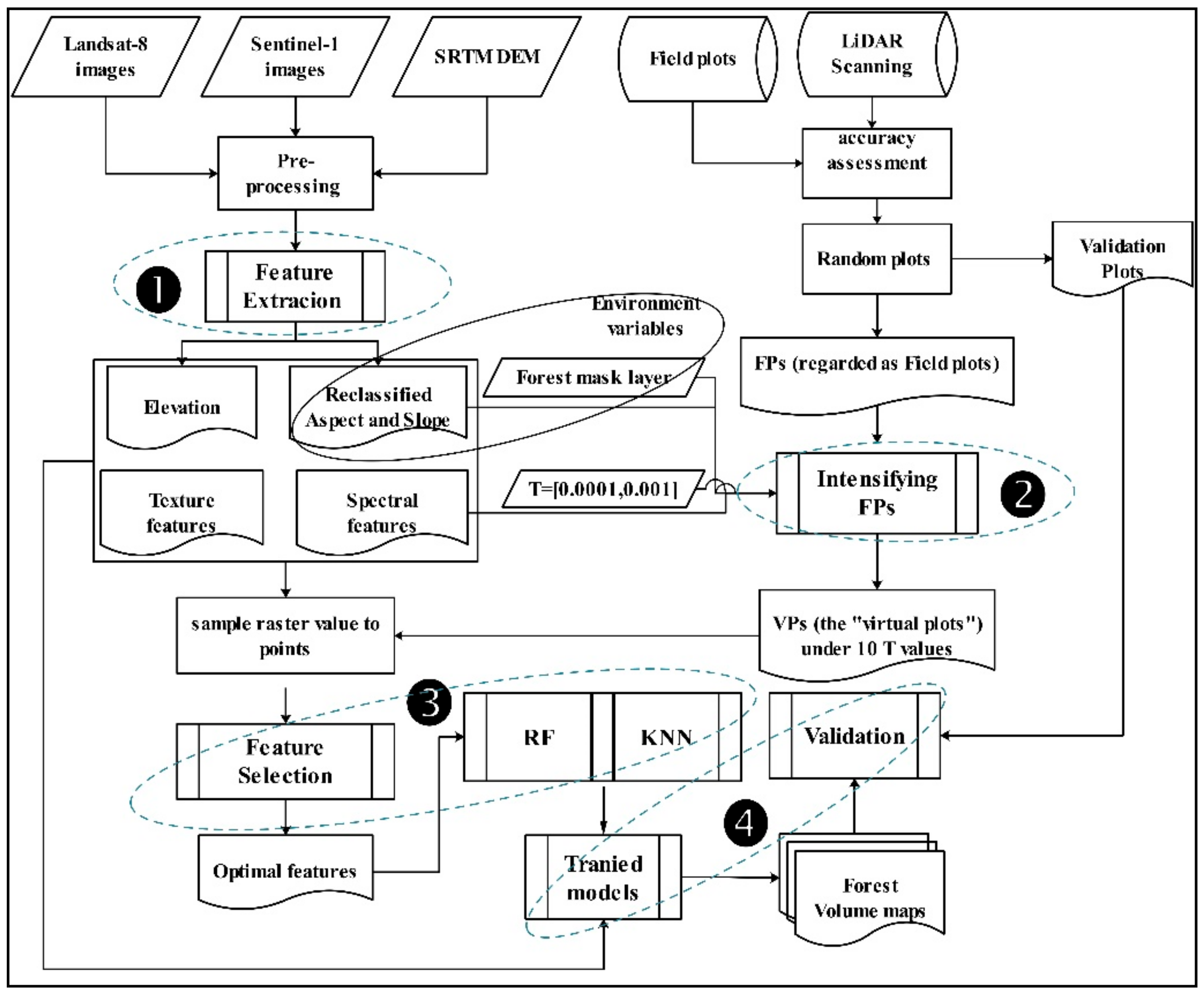
2. Materials and Methods

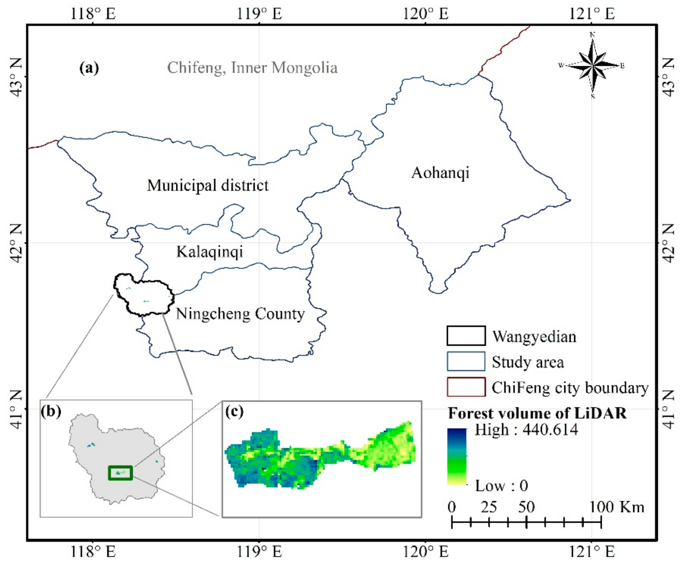
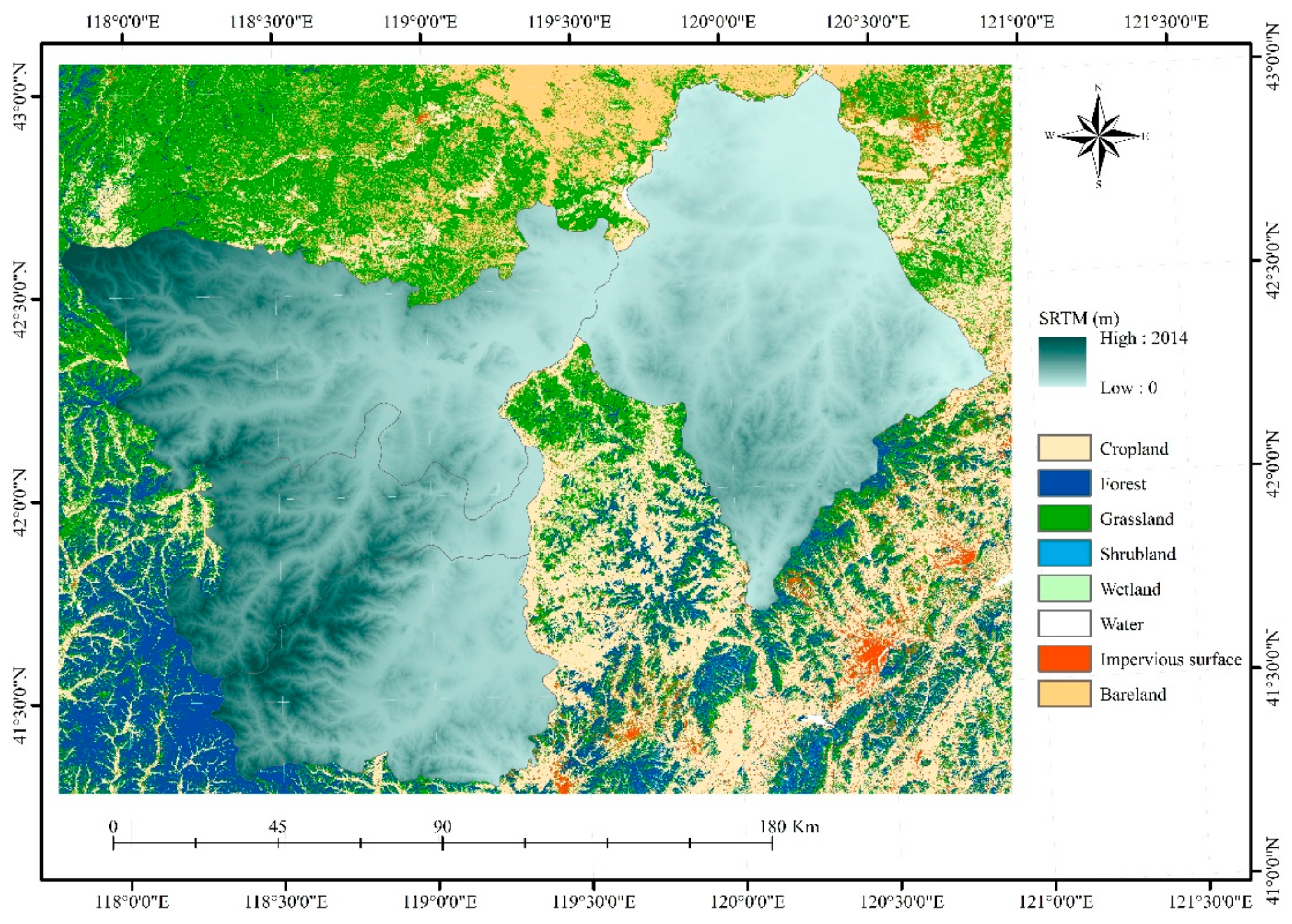
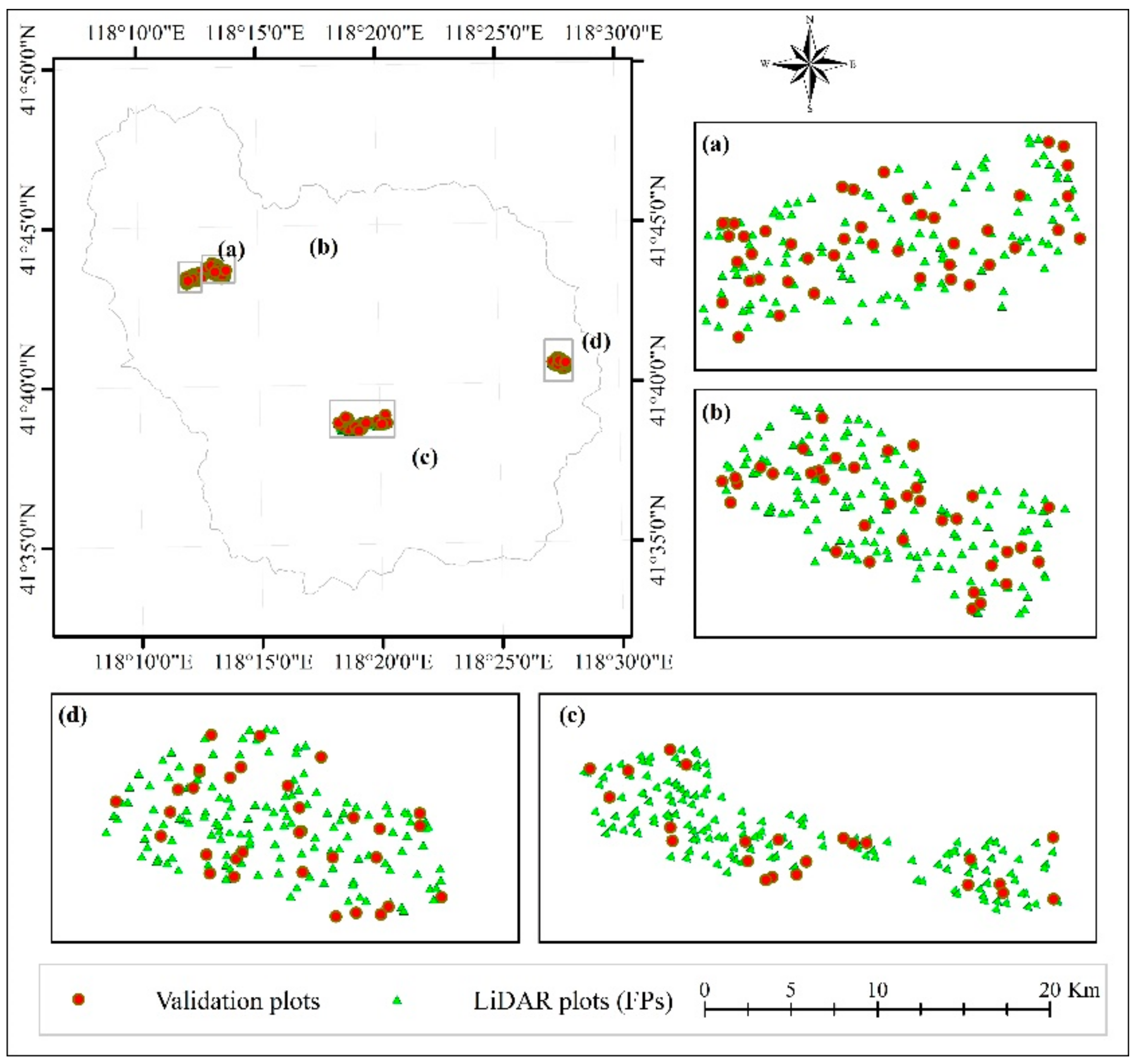
2.1. Chifeng City, Inner Mongolia

The study area is located in the east of Inner Mongolia, covering four administrative regions of Chifeng city (municipal district, Aohanqi, Kalaqinqi, and Ningcheng County) (Figure 1), which has complex and diverse topography with an elevation ranging from 300 m to 2000 m, and small mountain flat land, as well as alluvial plain scattering along the river. The climate of this area is temperate semi-arid continental monsoon climate zone, the average annual temperature in most areas is 0–7 °C increasing from northwest to southeast, and the annual average precipitation is 381 mm. Additionally, Chifeng also has abundant forest resources, and plantations of pine, poplar, and some other shrubbery dominated the whole study area.

2.2. Data Collection

2.2.1. Landsat-8 OLI & Sentinel-1A

Optical and SAR satellite images were used for regional remote sensing applications. The whole image collection consists of Landsat-8 and Sentinel-1A, which were acquired through Google Earth Engine (GEE) (https://code.earthengine.google.com/) cloud platform with a restricted study area [48]. GEE provides powerful computing capabilities and convenient access to satellite data, but also mature machine learning algorithms [49,50,51]. We generated Landsat-8 surface reflectance (SR) images composites via atmospheric correction operation while using the Land Surface Reflectance Code (LaSRC) implemented in GEE [52], of which four visible and near-infrared (VNIR) bands and two short-wave infrared (SWIR) bands were selected for subsequent analysis, because these bands have been found to depict forest characteristics in a number of studies [53,54,55], and Sentinel-1A radar backscatter composites from a dual-polarization C-band SAR instrument was processed while using the Sentinel-1 Toolbox to generate a calibrated, ortho-corrected product for 2017. The SR composite value was the greenest pixel from the eight scenes, where the greenest pixel means the pixel with the highest value of the Normalized Difference Vegetation Index (NDVI) (

Table 1. Details of Landsat-8 and Sentinel-1A satellites data.

Sensor Type	Acquisition Dates (Year-Month-Day)	Number of Scenes
Landsat-8 OLI	2017-09-21	2
	2017-09-23	1
	2017-09-28	2
	2017-09-30	3
Sentinel-1A	2017-09-23	2
	2017-09-24	2
	2017-09-28	1
	2017-09-30	2

).

2.2.2. Forest Volume Maps of LiDAR and Field Plots

The forest volume that was extracted by UAV LiDAR data was acquired from 22 to 24 September 2017 representing the close enough date as compared to the sensing date of the optical and radar images. The data consist of four patches that are distributed in Wangyedian forest districts (Figure 1) and were regarded as reference and validation for further analysis. A total of 17 field plots from 21 to 28 September 2017 were also obtained in relation to UAV LiDAR acquisitions to accomplish accuracy assessment of the original LiDAR scanning, which is the critical basis of this study. The consistent time was to ensure the reliability of the verification results.

2.2.3. Topographic Data

The Shuttle Radar Topography Mission (SRTM) (http://srtm.csi.cgiar.org/srtmdata/) was a National Aeronautics and Space Administration (NASA) mission undertaken in 2000 to enable accessing elevation data from 56°S to 60°N (over 119 million km², covering more than 80% of the global surface), which produced high-precision (one arc-second, or around 30 m) digital surface elevation models (DSM) from 9.8 terabytes C-band radar images that were obtained by the Endeavour Space Shuttle from 11–22 February while using radar mapping technology [56]. It has been providing a reliable source of data for geoscience analysis at global and regional scales as one of the world’s most complete high-precision terrain data [57,58,59]. The restricted administrative divisions using ArcGIS software were utilized to clip topographic data. The western elevation of the entire study area is higher than that of the eastern regions, and the highest elevation value from the SRTM of the study area is about 2000 m (Figure 2).

2.2.4. Auxiliary Data

Finer Resolution Observation and Monitoring of Global Land Cover (FROM-GLC30) is the first 30 m resolution global land cover maps that were produced using Landsat Thematic Mapper (TM) and Enhanced Thematic Mapper Plus (ETM+) data by Tsinghua University [60]. The Land Cover classification of which the detailed information that is given in

Table 2. The classification system of FROM-GLC30.

Name	Code
Cropland	1
Forest	2
Grassland	3
Shrubland	4
Wetland	5
Water	6
Tundra	7
Impervious surface	8
Bareland	9
Snow/Ice	10

was downloaded from the website (http://data.ess.tsinghua.edu.cn/fromglc2017v1.html) and used as a mask layer to enable us to directly access the spatial distribution of forest in the selection of restricted data over forest layer.

2.3. Methods

The overall workflow consists of the following four processes: (1) Extracting features from Landsat-8 and Sentinel-1; (2) intensifying points of forest volume that were derived from LiDAR mapping to generate training and validation samples; (3) feature selection and model training for RF and KNN algorithm; and, (4) estimating forest volume and assessing the accuracy of outcomes. Figure 3 shows the specific technical process.

2.3.1. Features Extraction from the Satellite Data

The surface reflectance and radar backscatter were further processed to spectral or texture indicators more relevant to forest volume in ENVI software. Six vegetation indices (NDVI, EVI, DVI, RVI, SAV, and MASI) were extracted from the Landsat-8 surface reflectance data to reflect the spectral characteristics of forest volume. Six texture predictor variables (mean, variance, homogeneity, contrast, dissimilarity, entropy, second moment, and correlation) were obtained for each band of Landsat-8 and Sentinel-1 data while using co-occurrence method for 3 × 3 windows using ENVI software, which resulted in a total of 64 texture features, of which 48 features from the six bands of Landsat-8, and the others from the two Sentinel-1 bands. We have also used Principal Component Analysis (PCA) for the six bands of Landsat-8, and the first two components were considered. For the topographic feature, three features (elevation, slope, and aspect) were acquired from the 30m-resolution SRTM data, and the reclassification was conducted for the slope and aspect variable based on the prior knowledge of forestry investigation that has been used in many field works (https://wenku.baidu.com/view/f4f111280066f5335a812134.html), where the slope was divided into six levels, and the aspect was reclassified into three categories (

Table 3. Slope and Aspect reclassification criteria.

Slope Levels			Aspect Categories
Value (°)	Name	Flag	Value (°)	Name	Flag
5	flat	0	−2–0	Flat| non-directional	0
5–14	gentle	1	0–22.5	North|Shady	1
15–24	slope	2	337.5–360	North|Shady	1
25–34	Steep	3	292.5–337.5	NorthWest|Shady	1
35–44	Acute	4	22.5–67.5	NorthEast|Shady	1
45	Dangerous	5	67.5–112.5	East|Sunny	2
			112.5–157.5	SouthEast|Sunny	2
			157.5–202.5	South|Sunny	2
			202.5–247.5	SouthWest|Sunny	2
			247.5–292.5	West|Sunny	2

).

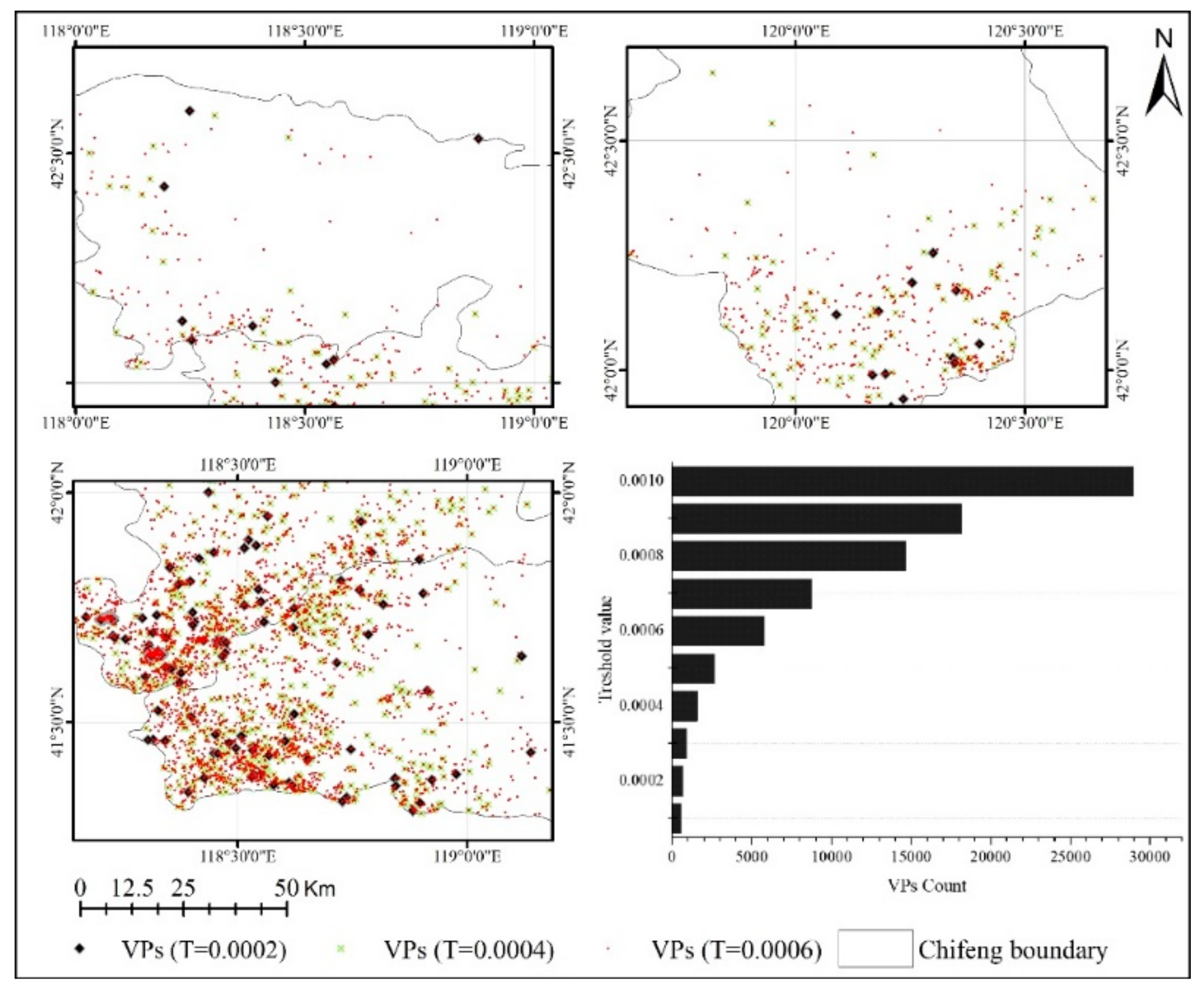
2.3.2. Expanding of LiDAR samples

The forest volume has been extracted from LiDAR data in the Wangyedian forest district to produce training and validation. We firstly made an accuracy assessment of the original LiDAR scanning results while using the 17 field plots. We used the toolbox (create random point integrated in ArcGIS) to yield 666 forest reference plots from the 30m-resolution forest volume using LiDAR, of which 134 plots served as validation samples to assess the results for the further analysis, and 532 plots functioned as field plots (FPs refer to plots that were obtained by sampling LiDAR images and functioned as real field plots) used for subsequent virtual plots (VPs refer to the intensified plots using FPs) generation (Figure 4).

We expanded the original FPs based on the raster features to obtain more plots to study the correlation between the satellite image features and FPs. According to the similarity criterion, two types of variables were involved: one was environment variables, being made up of reclassified aspect, slope, and the forest mask layer from FROM-GLC30, and the other was remotely sensed variables, consisting of four VNIR bands were considered to the FPs expanding operation. First, we extracted the value of the pixel of the environment, as well as remote sensing, features overlapping each FP, which was repeated for all FPs, and we then searched for the most similar pixels (MSPs) throughout the study area. The FP and MSPs have to satisfy two conditions: environmental values equal to those of the FP, which means that they belong to the same surroundings with the given FP, and their remotely sensed values should be close enough to FP that means the spectral difference cannot exceed to the given threshold value. Such conditions indicate their spectral and texture information reflected by satellite images is similar to the given FP [46], as:

$$\left\{\begin{array}{ll}{\mathrm{MSP}}_{\mathrm{s}}{(\mathrm{e}}_{\mathrm{i}}{)=\mathrm{FP}(\mathrm{e}}_{\mathrm{i}})\hfill & (\mathrm{i}=1,2,3)\hfill \\ {|\mathrm{MSP}}_{\mathrm{s}}{(\mathrm{r}}_{\mathrm{j}}{)-\mathrm{FP}(\mathrm{r}}_{\mathrm{j}}\left)\right| < \mathrm{T} \hfill & (\mathrm{j}=1,2,3,4)\hfill \end{array}\right.$$

(1)

where e and r represent the environment and remotely sensed variables respectively, and the subscripts i and j indicate their corresponding index numbers. T denotes the threshold value that is used to quantify the spectral closeness; to find the optimal T value, we initialized the threshold in an interval [0.0001, 0.001], yielding a total of 10 threshold values. The threshold range was given in consideration of the one-sidedness and subjectivity of a single threshold, and it was inspired by previous related studies on measurement of spectral closeness of Landsat-5, where a fixed threshold (0.01) was given [47]. As we all know that if the threshold is too lenient, the VPs would be very error-prone. Therefore, we took 0.01 as the maximum threshold and try to find a better threshold.

When all of the MSPs were identified for a certain FP, the value of FP was directly assigned to the MSPs, and the MSPs were then turned into VPs. A total of 10 sets of VPs corresponding to the given 10 T values were acquired at last.

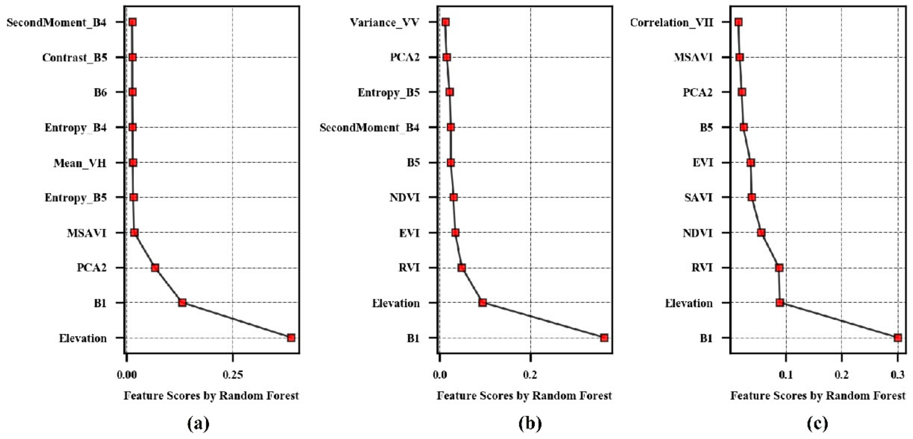
2.3.3. Feature Selection and Modeling

RF [61,62] and KNN [63] were adopted to model the relationship between forest volume value and remotely sensed features. For RF, it is based on a large number of the tree structure and is regarded as an easy-to-use algorithm, because its intuitive and understandable hyper-parameters usually produce a good prediction result by default. The KNN algorithm is also a mature and simple machine learning algorithm that assigns the average of the properties of these neighbors to the sample by finding its k nearest neighbors. For training samples, there were 10 sets of VPs samples with different numbers being generated by threshold values, together with one set of FPs, yielding 21 sets of sample combinations (the number of combination FPs, FPs + VPs, and VPs was 10, 10, and one, respectively).

The feature selection and model training processes were produced from the combinations using the “scikit-learn” package in the python programming language. The feature selection performance was carried out for 83 candidate features, and the optimal 10 features were selected by ranking their importance based on mean decrease Gini (MDG) criteria for subsequent modeling. A predictor variable that has the maximum MDG value is of the most importance. We have used both RF and KNN models and applied the grid searching methodology for detecting the optimal values of key hyper-parameters for the two models to estimate the reliable forest volume distribution.

Table 4. Configuration for hyperparameters both in RF and KNN modeling.

Algorithm Type	Hyperparameter Name	Interval	Step Length
RF	n_estimators	[10,60]	3
	max_depth	[1,35]	2
KNN	n_neighbors	[2,15]	1
	weights	[‘uniform’, ‘distance’]
	p	[1,4]	1

describes the configuration for key hyper-parameter optimization.

2.3.4. Forest Volume Mapping and Validation

A total of 20 regional forest volume mapping results were generated for the 10 T values based on trained models combined with the best 10 feature variables, and the mapping accuracy was evaluated while using a stand-alone validation dataset composed of 134 LiDAR points (Figure 4). We have also computed the root mean square error (RMSE) and mean absolute error (MAE) to quantify the error in the estimation of forest volume, as:

$$\mathrm{RMSE}=\sqrt{\frac{1}{\mathrm{n}}{\displaystyle \sum _{i=1}^n{{(\mathrm{y}}_{\mathrm{i}} -\hat{\mathrm{y}})}^2}}$$

(2)

and

$$\mathrm{MAE}=\frac{1}{\mathrm{n}}{\displaystyle \sum _{\mathrm{i}=1}^{\mathrm{n}}{|\mathrm{y}}_{\mathrm{i}}-\hat{\mathrm{y}}|}$$

(3)

where ${\mathrm{y}}_i$ denotes the measured and predicted volume values of points i and $\hat{\mathrm{y}}$ represents the mean value for all of the measured validation points. The n is the number of validation samples and equals to 134 here. The RMSE and MAE were compared while using RF and KNN models.

3. Results

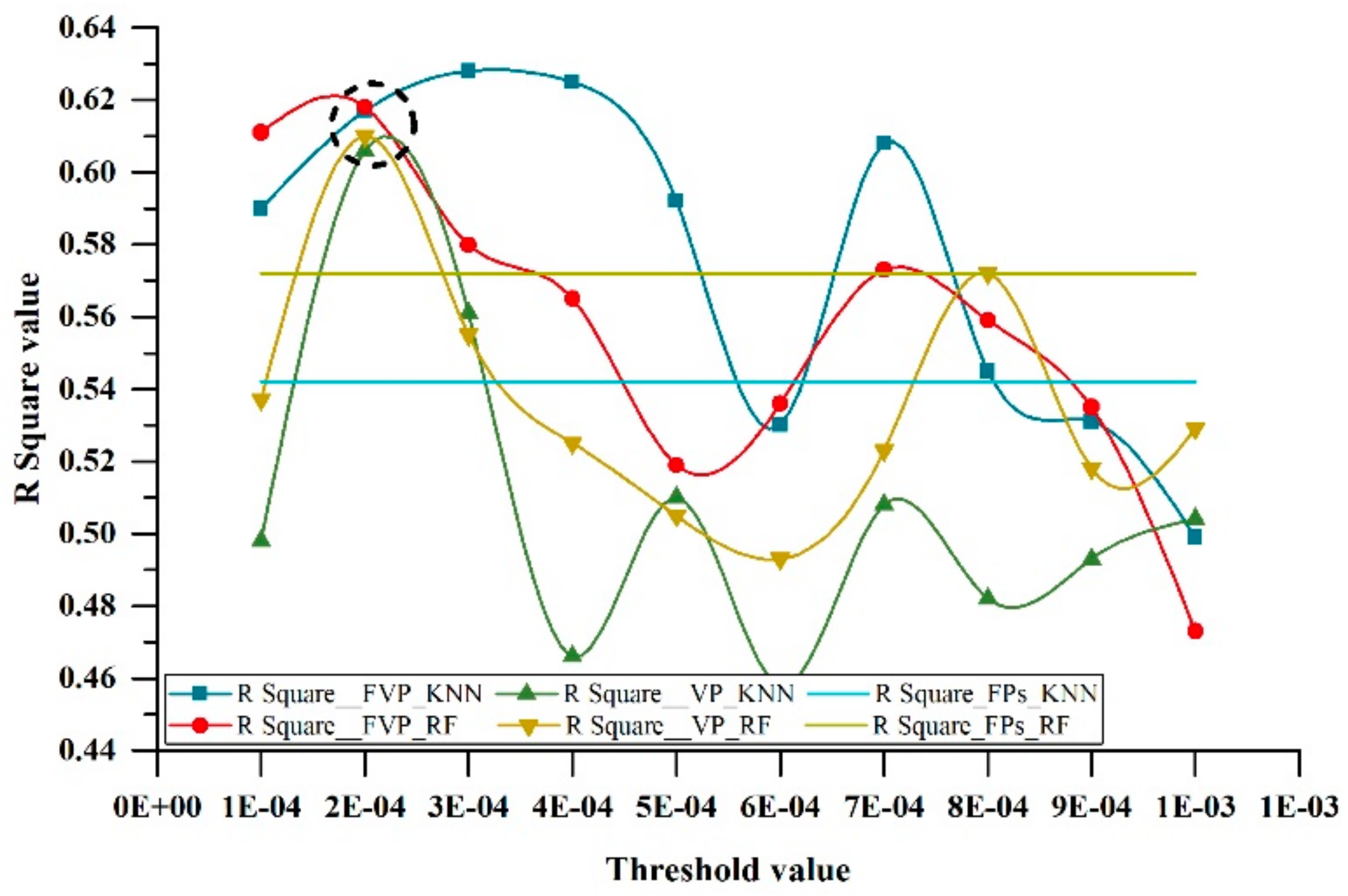
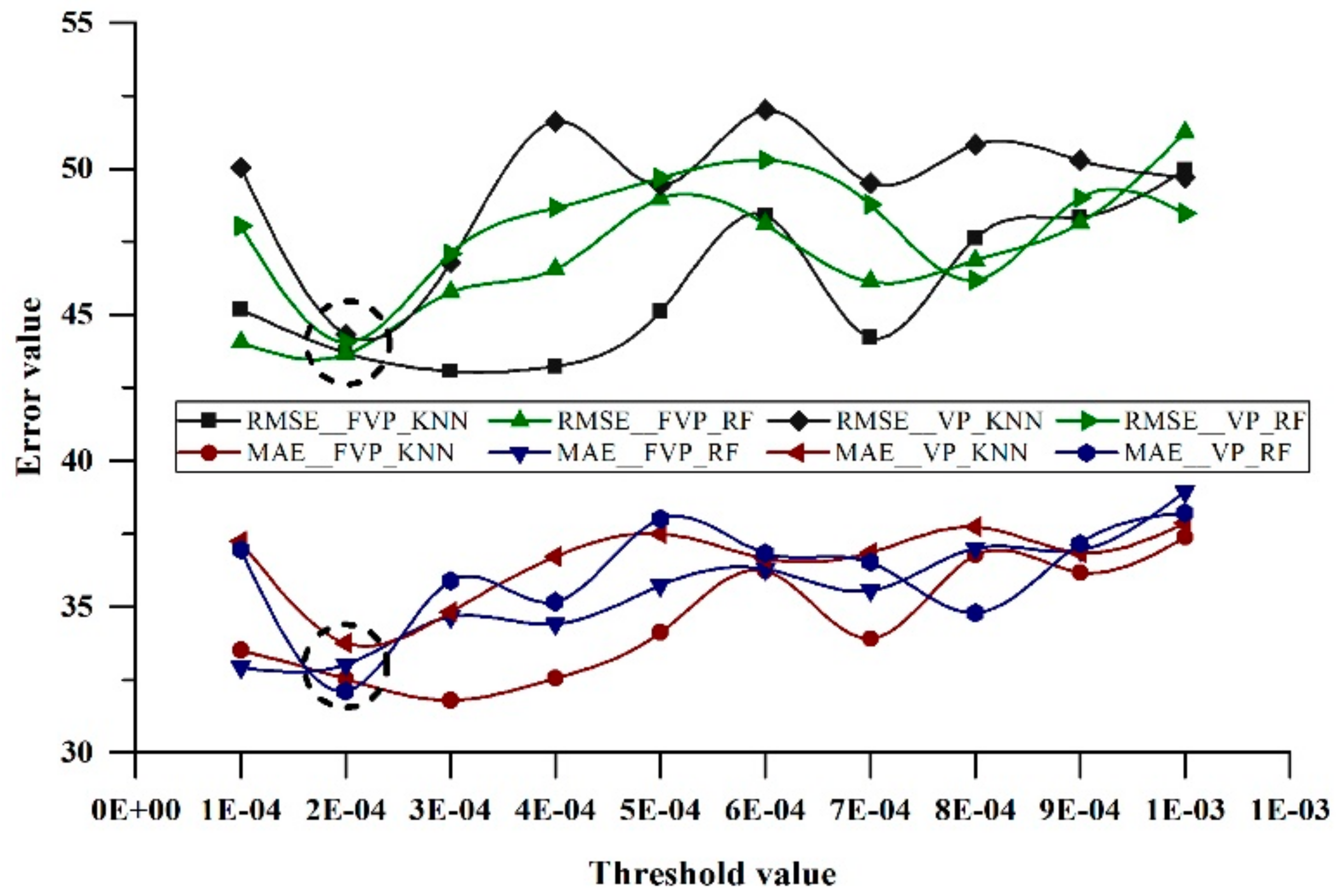
3.1. Expanding of LiDAR Samples

More abundant samples were produced while using FPs that were derived from LiDAR mapping combined with remote sensing and topographic images.

Table 5. Accuracy assessment table of forest volume map of UAV LiDAR.

Location		Forest Volume Value (m3/ha)		Accuracy Assessment
Lat	Lon	Ground Truth Value	LiDAR Estimation
41.7257	118.2260	198.93	204.10	26.89 m3/ha (RMSE) 0.76 (R Squared) 84.10% (accuracy)
41.7257	118.2270	191.19	198.52
41.7260	118.2180	279.40	239.36
41.7265	118.2210	187.47	174.14
41.7276	118.2130	324.08	208.35
41.7295	118.2150	218.26	160.37
41.6472	118.3310	64.39	51.74
41.6468	118.3320	63.13	58.78
41.6463	118.3340	57.68	62.02
41.6473	118.3330	55.12	57.94
41.6467	118.3220	154.63	160.63
41.6463	118.3240	159.58	171.90
41.6467	118.3240	93.74	179.40
41.6454	118.3180	251.41	224.48
41.6461	118.3190	229.69	224.30
41.6455	118.3090	233.76	185.30
41.6462	118.3110	204.70	195.90

Note: RMSE, Lat, and Lon refers to the root mean square error, Latitute, and Longitude.

depicts the accuracy assessment of the original LiDAR scanning, from which the accuracy of forest volume measurement by LiDAR estimation against ground truth can be seen from the statistical values (RMSE and R²), and the contingency matrix also shows that the LiDAR estimation accuracy is above 84%. The intensified sample distribution was restricted within the entire study area (Figure 5), working out more reasonable and representative for regional forest volume estimation when compared with the original LiDAR samples that were concentrated in one forest district. As Figure 5 shows, the spatial frequency of VPs increased with the increasing threshold value. Additionally, we have carried out statistical analysis using a bar chart with the horizontal and vertical axis denoting the expanded sample number and threshold value to understand the distribution of the number of each expanded point for different thresholds.

3.2. Feature Importance and Modeling

We have carried out detailed statistics for 83 candidate features while using mean decrease Gini (MDG) measures that were embedded into the RF algorithm. The expanding samples procedure produced a total of 21 extrapolated sample combinations, but we plotted the most important 10 variables that had the highest MDG values of three combinations using line chart, of which the vertical axis listed the best feature name, and the horizontal axis represented the score that was measured by MDG. The most significant feature was a topographic variable (i.e., Elevation) from all the inputting variables using only FPs samples (e.g., the left subgraph). Whereas the blue band of Landsat-8 demonstrated higher contribution over the others to the volume prediction while using two different sample combinations (i.e., FPs + ${\mathrm{VPs}}_{(\mathrm{T}=2\times {10}^{-4})}$ and ${\mathrm{VPs}}_{(\mathrm{T}=2\times {10}^{-4})}$ generated by expanding LiDAR samples at a given threshold value (2 × 10⁻⁴). Besides, the two combinations yielded the same top three important features (B1, Elevation, and RVI, respectively) that reached a similarity of 70% (e.g., the middle and right subgraphs). In addition, the optimal features of FPs contained more texture variables when compared to the other two combinations (Figure 6).

The model training step of RF and KNN was carried out based on the previously selected 10 features, and the grid-searching implements determined all of the optimal values for hyper-parameters of models under 10 different threshold conditions (i.e., from 1 × 10⁻⁴ to 1 × 10⁻³ in 1 × 10⁻⁴ step length). The resulting optimal models were used in the volume estimation.

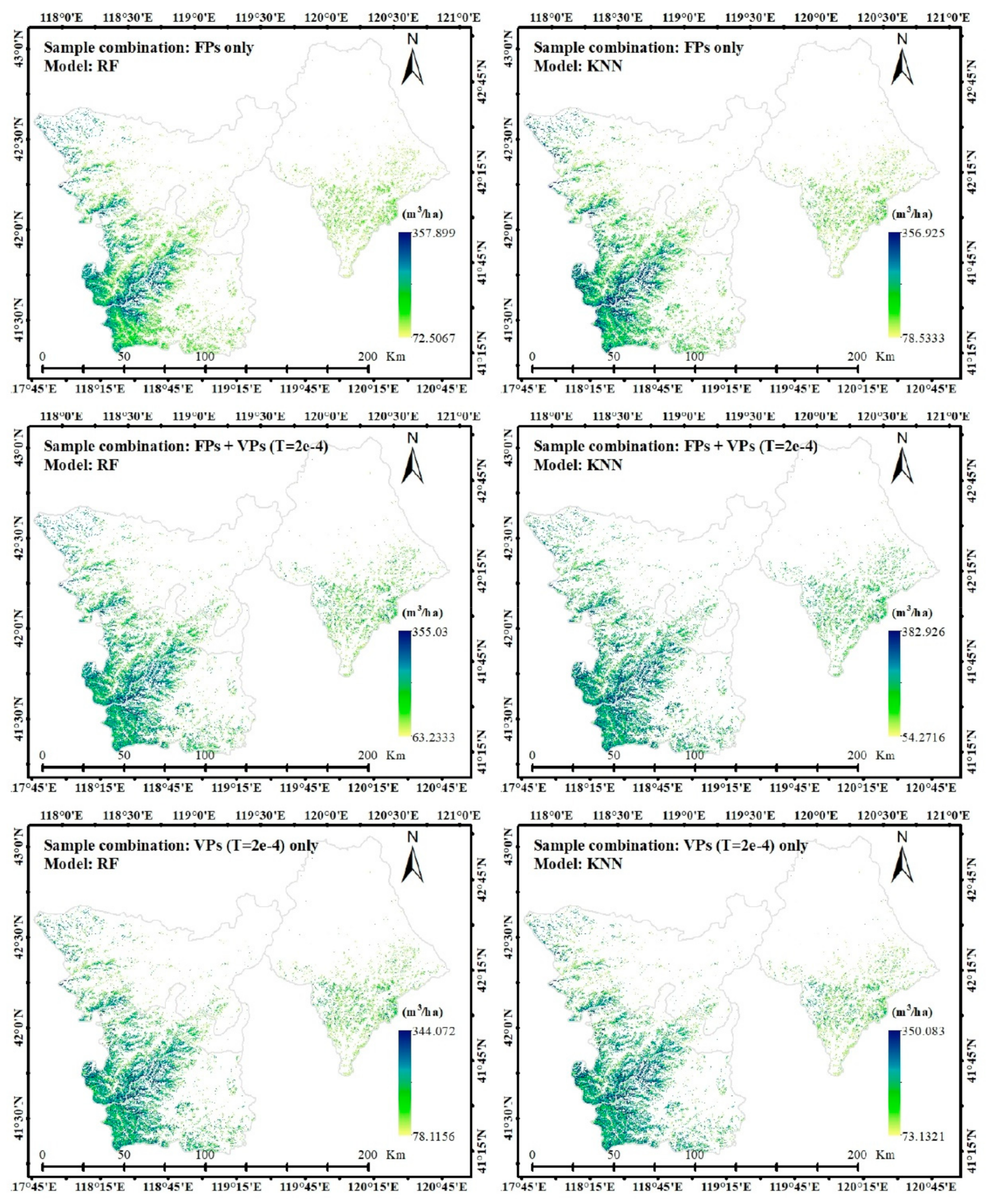
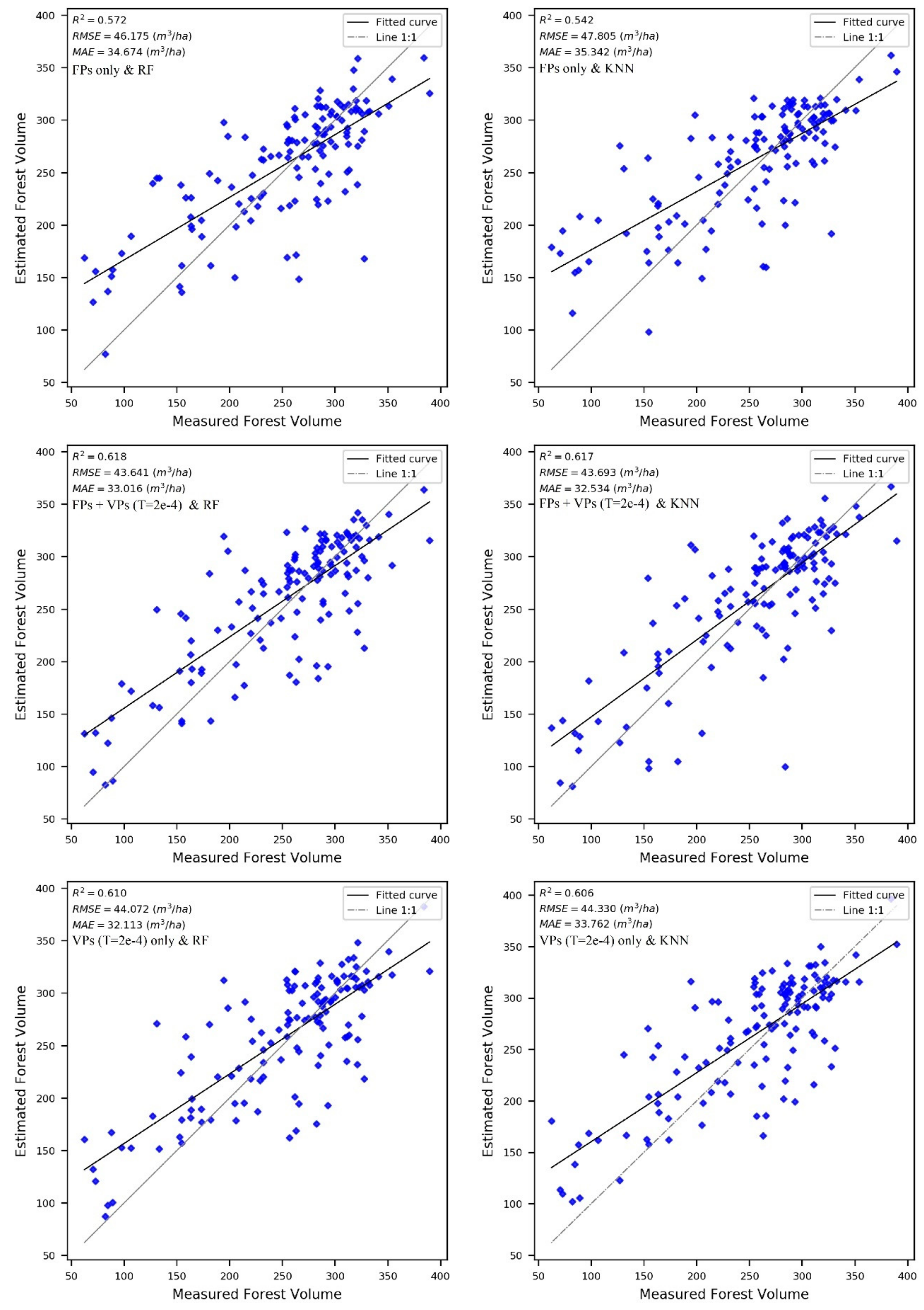
3.3. Optimal Forest Volume Estimation and Validation

The forest volume mappings were produced while using the two trained models, and the results were evaluated using the validation samples (Figure 4). All of the selected sample combinations were separately entered into RF and KNN model to carry out the estimation process. According to accuracy validation, the variation of the R squared value is shown in Figure 6. All of the variations show an increase after decreasing rapidly, and the highest precisions were obtained at the peak point of T = 2 × 10⁻⁴, where the R squared values were found to be more than 0.6, higher than using only FPs combination (two horizontal lines). In addition, the accuracy of the same model, taking the RF model as an example, was found to be consistent under the driving of the two sample combinations, (i.e., FVP and VP), and additionally adding the original sample (FVP, red curve) shows a better performance, and its accuracy was found to be higher than that of only using the extended sample (VP, yellow curve). When compared with the KNN model, this difference in the accuracy of different sample composites that were generated by the random forest model was smaller, indicating that the random forest model was more stable and robust to forest volume estimation (Figure 7). The root mean square error (RMSE) and mean absolute error (MAE) variations agree with the R squared value.

We have considered the RF and KNN models to estimate the highest precision results of forest volume distribution containing three groups, of which each was made up of two mappings from the corresponding models (Figure 8), and we also conducted an accuracy assessment while using the validation samples (Figure 9). The results show that the forest volume across the study area varies from 50 to 360 m³/ha, and spatial distribution shows the difference between original samples (FPs only) and additionally adopting expanded samples (i.e., $\mathrm{V}\mathrm{P}\mathrm{s}{}_{(\mathrm{T}=2\times {10}^{-4})}$₎ only and FPs + $\mathrm{V}\mathrm{P}\mathrm{s}{}_{(\mathrm{T}=2\times {10}^{-4})}$). For the former, the high values were mainly concentrated in the west of the Kalaqinqi and Ningcheng county, while they were also distributed in the south of Aohanqi with the adding of VPs. The scatter plot shows that expanding the FPs collection can potentially improve the accuracy of the outcome when compared to the use of only FPs. The RF model using the VPs only combination performed a better precision result than that driven by only FPs; the result was further improved (R² = 0.618, RMSE = 43.641 m³/ha, and MAE = 33.016 m³/ha) by combining of FPs with VPs (i.e., FPs + VPs) while using the RF model. The accuracy trend using the KNN model was similar to the RF, and the accuracy of the outcomes of the two models was almost the same for the same sample combination, reaching the highest accuracy (R² = 0.617, RMSE = 43.693 m³/ha, and MAE = 32.534 m³/ha). The accuracy for the forest volume distribution was almost same (R² = 0.62, RMSE = 43 m³/ha, and MAE = 32 m³/ha) with the comparison of two models.

4. Discussion

The expanding forest volume samples resulted in more abundant samples that were rationally distributed throughout the entire study area, which can especially alleviate the shortage of ground- truth samples for forest attributes calculation in large areas while using machine learning [47]. We achieved regional forest volume estimation while using RF and KNN algorithms that have been widely used both in classification and regression [64,65,66,67]. Related studies directly imputed forest volume combining Landsat images and forest inventory data using KNN model, yielding a result with highest precision (RMSE = 74 m³/ha) [68]. The accuracy of forest volume estimation could be improved (RMSE = 62 m³/ha) when LiDAR was used with other multi-source remote sensing data [40]. When compared with existing related research, our method achieves an accuracy improvement (RMSE = 44 m³/ha), and it reduces the dependence on the amount of LiDAR data. We have found two critical procedures, one is sample expanding, and the other is feature selection, which is involved in the following discussions.

4.1. Samples Extrapolation

The low cost-effectiveness and time-consuming approach to acquire enough forest field measurements that, however, are important to regional forest applications, especially when a nonparametric method is considered. We considered three satellite-acquired topographic variables, i.e., elevation, aspect, and slope, which were different from the earlier studies, where more climatic variables (temperature, precipitation, and solar radiation) were required [46]. The threshold value, used for spectral similarity measure to find MSPs at a given original point, was not a single fixed value; instead, it was assigned within an interval to identify the optimal one, which resulted in more sample combinations for subsequent procedures discussed earlier. The larger the threshold, the more extended samples size were produced (Figure 5), whereas, the change in accuracy was not linearly positively correlated to the number of extended samples (Figure 7 and Figure 10), which means that the accuracy of outcomes, besides the quantity, was also related to the correlation among the samples. For satellite auxiliary data, the primary surface reflectance of four VNIR bands of Landsat-8 was used, by which many indices were designed for vegetation studying, and we will try to involve more data, such as L-band radar backscatter being found to be more sensitive to forest attributes in the future study [69].

4.2. Feature Importance Measure

It is of great importance to select variables before modeling nonparametric methods due to the existence of covariates in satellite data [70]. The contribution of features to forest volume was evaluated while using MDG measures, which were embedded in RF algorithm, in which the changes of Gini impurity metric was calculated and ranked, and the MDG methodology has been applied for selecting features derived from air- and space- images and was demonstrated to be popular, robust, and stable for feature importance measure [71,72,73,74,75,76]. Moreover, the feature selection process was performed for each sample combination, and the variations of the results (Figure 6) show that the quantity of sample affected the variable importance measurement. We need to take additional criteria for improving feature selection in our future studies.

4.3. Implications and Future Work

The overall accuracy (Figure 8 and Figure 9) of this study has proven the feasibility of the proposed method that would be very helpful in the acquisition of forest structure parameters. Thus, future work could acquire reliable regional forest volume distribution at a relatively low cost by intensifying the UAV-LiDAR data. The following aspects could affect the results in this study. First, the existence of positioning error of the original LiDAR plots and remotely sensed data would cause some deviations in outcomes, of which the improvement depends on the equipment and data processing methods. Besides, adding ground-measured samples to the accuracy verification comparison could further improve the reliability of the results. Additionally, the validity of the feature directly affects the results, the aspect and slope are directly input into model, while the sine and cosine transformations were also used in related studies [77]. For non-parametric models, the initialization of hyperparameters has a significant influence on the model output, the key hyper-parameters of RF and KNN are given in Table 4 in insofar study, but they vary with the specific problem being dealt with. Thus, our further work would consider using additional ground truth field plots to validate the results and analyze whether the interactions between different topographic variables and terrain components affect the results. In addition, we would also pay attention to hyper-parameters tuning of machine learning algorithms, and further analyze its influence on final model output.

5. Conclusions

In the present study, regional forest volume mappings at a resolution of ~30 m were produced based on the point-specific plots that were extracted from LiDAR scanning images combined with the expanded samples, Landsat-8, Sentinel-1, and topographic images. It is a challenging but rewarding way to use the LiDAR data within a limited distribution range for generating quantitative forest attributes at a moderate geographic scale. The forest volume was in the range of 50–360 m³/ha; besides, the results with the highest accuracy were produced. Our results show a stable performance (R² = 0.62, RMSE = 43 m³/ha, and MAE = 32 m³/ha) over the RF and KNN models. Meanwhile, the optimal threshold value was found to be given 2 × 10⁻⁴ in the range from 1 × 10⁻⁴ to 1 × 10⁻³ in the intervals of 1 × 10⁻⁴.

The present study proposed a promising approach for producing forest volume mapping combined with multi-source remotely sensed data via expanding the original samples that have a limited number or distribution. Therefore, the proposed methodology could be incorporated into forest resource survey and monitoring programs to assist in the quantitative measurement of forest properties to fully exploit the advantages of satellite technology and reduce the time and labor costs of traditional surveys.

References

1. Dixon, R.K.; Brown, S.; Houghton, R.A.; Solomon, A.M.; Trexler, M.C.; Wisniewski, J. Carbon Pools and Flux of Global Forest Ecosystems. Science 1994, 263, 185–190. [Google Scholar] [CrossRef] [PubMed]
2. Bonan, G.B. Forests and climate change: Forcings, feedbacks, and the climate benefits of forests. Science 2008, 320, 1444–1449. [Google Scholar] [CrossRef] [PubMed] [Green Version]
3. Coomes, D.A.; Allen, R.B. Mortality and tree-size distributions in natural mixed-age forests. J. Ecol. 2007, 95, 27–40. [Google Scholar] [CrossRef]
4. Magnussen, S.; Naesset, E.; Gobakken, T. Prediction of tree-size distributions and inventory variables from cumulants of canopy height distributions. Forestry 2013, 86, 583–595. [Google Scholar] [CrossRef] [Green Version]
5. Saarinen, N.; Kankare, V.; Vastaranta, M.; Luoma, V.; Pyorala, J.; Tanhuanpaa, T.; Liang, X.L.; Kaartinen, H.; Kukko, A.; Jaakkola, A.; et al. Feasibility of Terrestrial laser scanning for collecting stem volume information from single trees. ISPRS J. Photogramm. Remote Sens. 2017, 123, 140–158. [Google Scholar] [CrossRef]
6. Cao, L.; Zhang, Z.N.; Yun, T.; Wang, G.B.; Ruan, H.H.; She, G.H. Estimating Tree Volume Distributions in Subtropical Forests Using Airborne LiDAR Data. Remote Sens. 2019, 11, 33. [Google Scholar] [CrossRef] [Green Version]
7. Santoro, M.; Cartus, O.; Fransson, J.E.S.; Shvidenko, A.; McCallum, I.; Hall, R.J.; Beaudoin, A.; Beer, C.; Schmullius, C. Estimates of Forest Growing Stock Volume for Sweden, Central Siberia, and Quebec Using Envisat Advanced Synthetic Aperture Radar Backscatter Data. Remote Sens. 2013, 5, 4503–4532. [Google Scholar] [CrossRef] [Green Version]
8. Ripple, W.J.; Wang, S.; Isaacson, D.L.; Paine, D.P. A Preliminary Comparison of Landsat Thematic Mapper and Spot-1 Hrv Multispectral Data for Estimating Coniferous Forest Volume. Int. J. Remote Sens. 1991, 12, 1971–1977. [Google Scholar] [CrossRef]
9. Tinkham, W.T.; Smith, A.M.S.; Affleck, D.L.R.; Saralecos, J.D.; Falkowski, M.J.; Hoffman, C.M.; Hudak, A.T.; Wulder, M.A. Development of Height-Volume Relationships in Second Growth Abies grandis for Use with Aerial LiDAR. Can. J. Remote Sens. 2016, 42, 400–410. [Google Scholar] [CrossRef]
10. Lefsky, M.A.; Cohen, W.B.; Acker, S.A.; Parker, G.G.; Spies, T.A.; Harding, D. Lidar remote sensing of the canopy structure and biophysical properties of Douglas-fir western hemlock forests. Remote Sens. Environ. 1999, 70, 339–361. [Google Scholar] [CrossRef]
11. Takahashi, T.; Yamamoto, K.; Senda, Y.; Tsuzuku, M. Predicting individual stem volumes of sugi (Cryptomeria japonica D. Don) plantations in mountainous areas using small-footprint airborne LiDAR. J. For. Res. 2005, 10, 305–312. [Google Scholar] [CrossRef]
12. Popescu, S.C. Estimating biomass of individual pine trees using airborne lidar. Biomass Bioenergy 2007, 31, 646–655. [Google Scholar] [CrossRef]
13. Popescu, S.C.; Zhao, K. A voxel-based lidar method for estimating crown base height for deciduous and pine trees. Remote Sens. Environ. 2008, 112, 767–781. [Google Scholar] [CrossRef]
14. Tonolli, S.; Dalponte, M.; Vescovo, L.; Rodeghiero, M.; Bruzzone, L.; Gianelle, D. Mapping and modeling forest tree volume using forest inventory and airborne laser scanning. Eur. J. For. Res. 2011, 130, 569–577. [Google Scholar] [CrossRef]
15. Strunk, J.L.; Reutebuch, S.E.; Andersen, H.E.; Gould, P.J.; McGaughey, R.J. Model-Assisted Forest Yield Estimation with Light Detection and Ranging. West. J. Appl. For. 2012, 27, 53–59. [Google Scholar] [CrossRef] [Green Version]
16. Tao, S.L.; Guo, Q.H.; Li, L.; Xue, B.L.; Kelly, M.; Li, W.K.; Xu, G.C.; Su, Y.J. Airborne Lidar-derived volume metrics for aboveground biomass estimation: A comparative assessment for conifer stands. Agric. For. Meteorol. 2014, 198, 24–32. [Google Scholar] [CrossRef]
17. Li, W.; Niu, Z.; Huang, N.; Wang, C.; Gao, S.; Wu, C.Y. Airborne LiDAR technique for estimating biomass components of maize: A case study in Zhangye City, Northwest China. Ecol. Indic. 2015, 57, 486–496. [Google Scholar] [CrossRef]
18. Tompalski, P.; Coops, N.C.; Marshall, P.L.; White, J.C.; Wulder, M.A.; Bailey, T. Combining Multi-Date Airborne Laser Scanning and Digital Aerial Photogrammetric Data for Forest Growth and Yield Modelling. Remote Sens. 2018, 10, 347. [Google Scholar] [CrossRef] [Green Version]
19. Lo, C.S.; Lin, C.S. Growth-Competition-Based Stem Diameter and Volume Modeling for Tree-Level Forest Inventory Using Airborne LiDAR Data. IEEE Trans. Geosci. Remote Sens. 2013, 51, 2216–2226. [Google Scholar] [CrossRef]
20. Falkowski, M.J.; Hudak, A.T.; Crookston, N.L.; Gessler, P.E.; Uebler, E.H.; Smith, A.M.S. Landscape-scale parameterization of a tree-level forest growth model: A k-nearest neighbor imputation approach incorporating LiDAR data. Can. J. For. Res.-Rev. Can. Rech. For. 2010, 40, 184–199. [Google Scholar] [CrossRef]
21. Silva, C.A.; Hudak, A.T.; Vierling, L.A.; Loudermilk, E.L.; O’Brien, J.J.; Hiers, J.K.; Jack, S.B.; Gonzalez-Benecke, C.; Lee, H.; Falkowski, M.J.; et al. Imputation of Individual Longleaf Pine (Pinus palustris Mill.) Tree Attributes from Field and LiDAR Data. Can. J. Remote Sens. 2016, 42, 554–573. [Google Scholar] [CrossRef]
22. Hickey, M.P.; Taylor, M.J.; Gardner, C.S. Full-wave modeling of small-scale gravity waves using Airborne Lidar and Observations of the Hawaiian Airglow (ALOHA-93) O(S-1) images and coincident Na wind/temperature lidar measurements (vol 107, pg 4357, 2002). J. Geophys. Res.-Atmos. 2002, 107. [Google Scholar] [CrossRef]
23. Xu, C.; Morgenroth, J.; Manley, B. Mapping Net Stocked Plantation Area for Small-Scale Forests in New Zealand Using Integrated RapidEye and LiDAR Sensors. Forests 2017, 8, 487. [Google Scholar] [CrossRef] [Green Version]
24. Xu, C.; Manley, B.; Morgenroth, J. Evaluation of modelling approaches in predicting forest volume and stand age for small-scale plantation forests in New Zealand with RapidEye and LiDAR. Int. J. Appl. Earth Obs. Geoinf. 2018, 73, 386–396. [Google Scholar] [CrossRef]
25. Tesfamichael, S.G.; van Aardt, J.A.N.; Ahmed, F. Estimating plot-level tree height and volume of Eucalyptus grandis plantations using small-footprint, discrete return lidar data. Prog. Phys. Geogr. 2010, 34, 515–540. [Google Scholar] [CrossRef] [Green Version]
26. Clementel, F.; Colle, G.; Farruggia, C.; Floris, A.; Scrinzi, G.; Torresan, C. Estimating forest timber volume by means of “low-cost” LiDAR data. Ital. J. Remote Sens. 2012, 44, 125–140. [Google Scholar] [CrossRef]
27. Palleja, T.; Tresanchez, M.; Teixido, M.; Sanz, R.; Rosell, J.R.; Palacin, J. Sensitivity of tree volume measurement to trajectory errors from a terrestrial LIDAR scanner. Agric. For. Meteorol. 2010, 150, 1420–1427. [Google Scholar] [CrossRef]
28. Lim, K.; Treitz, P.; Wulder, M.; St-Onge, B.; Flood, M. LiDAR remote sensing of forest structure. Prog. Phys. Geogr. 2003, 27, 88–106. [Google Scholar] [CrossRef] [Green Version]
29. Peterson, D.L.; Aber, J.D.; Matson, P.A.; Card, D.H.; Swanberg, N.; Wessman, C.; Spanner, M. Remote-Sensing of Forest Canopy and Leaf Biochemical Contents. Remote Sens. Environ. 1988, 24, 85–108. [Google Scholar] [CrossRef]
30. Collins, J.B.; Woodcock, C.E. An assessment of several linear change detection techniques for mapping forest mortality using multitemporal landsat TM data. Remote Sens. Environ. 1996, 56, 66–77. [Google Scholar] [CrossRef]
31. Carpenter, G.A.; Gjaja, M.N.; Gopal, S.; Woodcock, C.E. ART neural networks for remote sensing: Vegetation classification from Landsat TM and terrain data. IEEE Trans. Geosci. Remote Sens. 1997, 35, 308–325. [Google Scholar] [CrossRef] [Green Version]
32. Gu, H.Y.; Dai, L.M.; Wu, G.; Xu, D.; Wang, S.Z.; Wang, H. Estimation of forest volumes by integrating Landsat TM imagery and forest inventory data. Sci. China Ser. E-Technol. Sci. 2006, 49, 54–62. [Google Scholar] [CrossRef] [Green Version]
33. Tokola, T. The influence of field sample data location on growing stock volume estimation in landsat TM-based forest inventory in eastern Finland. Remote Sens. Environ. 2000, 74, 422–431. [Google Scholar] [CrossRef]
34. Mura, M.; Bottalico, F.; Giannetti, F.; Bertani, R.; Giannini, R.; Mancini, M.; Orlandini, S.; Travaglini, D.; Chirici, G. Exploiting the capabilities of the Sentinel-2 multi spectral instrument for predicting growing stock volume in forest ecosystems. Int. J. Appl. Earth Obs. Geoinf. 2018, 66, 126–134. [Google Scholar] [CrossRef]
35. Chrysafis, I.; Mallinis, G.; Tsakiri, M.; Patias, P. Evaluation of single-date and multi-seasonal spatial and spectral information of Sentinel-2 imagery to assess growing stock volume of a Mediterranean forest. Int. J. Appl. Earth Obs. Geoinf. 2019, 77, 1–14. [Google Scholar] [CrossRef]
36. Santoro, M.; Eriksson, L.; Schmullius, C.; Wiesmann, A. Seasonal and Topographic Effects on Growing Stock Volume Estimates from JERS-1 Backscatter in Siberian Forests; Millpress Science Publishers: Rotterdam, The Netherlands, 2004; pp. 151–158. [Google Scholar]
37. Santoro, M.; Wegmuller, U.; Askne, J. Forest stem volume estimation using C-band interferometric SAR coherence data of the ERS-1 mission 3-days repeat-interval phase. Remote Sens. Environ. 2018, 216, 684–696. [Google Scholar] [CrossRef]
38. Wang, C.L.; Niu, C.; Cong, P.F.; Lin, W.P.; Guo, Z.X.; IEEE. Retrieval Forest Stock Volume of Large Plantation in South China Using RADARSAT-SAR; IEEE: New York, NY, USA, 2005; pp. 3051–3054. [Google Scholar]
39. Wilhelm, S.; Huttich, C.; Korets, M.; Schmullius, C. Large Area Mapping of Boreal Growing Stock Volume on an Annual and Multi-Temporal Level Using PALSAR L-Band Backscatter Mosaics. Forests 2014, 5, 1999–2015. [Google Scholar] [CrossRef] [Green Version]
40. Cartus, O.; Kellndorfer, J.; Rombach, M.; Walker, W. Mapping Canopy Height and Growing Stock Volume Using Airborne Lidar, ALOS PALSAR and Landsat ETM. Remote Sens. 2012, 4, 3320–3345. [Google Scholar] [CrossRef] [Green Version]
41. Mauya, E.W.; Koskinen, J.; Tegel, K.; Hamalainen, J.; Kauranne, T.; Kayhko, N. Modelling and Predicting the Growing Stock Volume in Small-Scale Plantation Forests of Tanzania Using Multi-Sensor Image Synergy. Forests 2019, 10, 21. [Google Scholar] [CrossRef] [Green Version]
42. Steinmann, K.; Mandallaz, D.; Ginzler, C.; Lanz, A. Small area estimations of proportion of forest and timber volume combining Lidar data and stereo aerial images with terrestrial data. Scand. J. For. Res. 2013, 28, 373–385. [Google Scholar] [CrossRef]
43. Hawrylo, P.; Wezyk, P. Predicting Growing Stock Volume of Scots Pine Stands Using Sentinel-2 Satellite Imagery and Airborne Image-Derived Point Clouds. Forests 2018, 9, 274. [Google Scholar] [CrossRef] [Green Version]
44. Puliti, S.; Saarela, S.; Gobakken, T.; Stahl, G.; Naesset, E. Combining UAV and Sentinel-2 auxiliary data for forest growing stock volume estimation through hierarchical model-based inference. Remote Sens. Environ. 2018, 204, 485–497. [Google Scholar] [CrossRef]
45. Saarela, S.; Grafstrom, A.; Stahl, G.; Kangas, A.; Holopainen, M.; Tuominen, S.; Nordkvist, K.; Hyyppa, J. Model-assisted estimation of growing stock volume using different combinations of LiDAR and Landsat data as auxiliary information. Remote Sens. Environ. 2015, 158, 431–440. [Google Scholar] [CrossRef]
46. Huang, S.; Ramirez, C.; Kennedy, K.; Mallory, J. A New Approach to Extrapolate Forest Attributes from Field Inventory with Satellite and Auxiliary Data Sets. For. Sci. 2016, 63, 232–240. [Google Scholar] [CrossRef] [Green Version]
47. Huang, S.; Ramirez, C.; Conway, S.; Kennedy, K.; Kohler, T.; Liu, J. Mapping site index and volume increment from forest inventory, Landsat, and ecological variables in Tahoe National Forest, California, USA. Can. J. For. Res. 2017, 47, 113–124. [Google Scholar] [CrossRef] [Green Version]
48. Gorelick, N.; Hancher, M.; Dixon, M.; Ilyushchenko, S.; Thau, D.; Moore, R. Google Earth Engine: Planetary-scale geospatial analysis for everyone. Remote Sens. Environ. 2017, 202, 18–27. [Google Scholar] [CrossRef]
49. Lee, J.S.H.; Wich, S.; Widayati, A.; Koh, L.P. Detecting industrial oil palm plantations on Landsat images with Google Earth Engine. Remote Sens. Appl. Soc. Environ. 2016, 4, 219–224. [Google Scholar] [CrossRef] [Green Version]
50. Teluguntla, P.; Thenkabail, P.S.; Oliphant, A.; Xiong, J.; Gumma, M.K.; Congalton, R.G.; Yadav, K.; Huete, A. A 30-m landsat-derived cropland extent product of Australia and China using random forest machine learning algorithm on Google Earth Engine cloud computing platform. ISPRS J. Photogramm. Remote Sens. 2018, 144, 325–340. [Google Scholar] [CrossRef]
51. Xiong, J.; Thenkabail, P.S.; Gumma, M.K.; Teluguntla, P.; Poehnelt, J.; Congalton, R.G.; Yadav, K.; Thau, D. Automated cropland mapping of continental Africa using Google Earth Engine cloud computing. ISPRS J. Photogramm. Remote Sens. 2017, 126, 225–244. [Google Scholar] [CrossRef] [Green Version]
52. Vermote, E.; Justice, C.; Claverie, M.; Franch, B. Preliminary analysis of the performance of the Landsat 8/OLI land surface reflectance produc t. Remote Sens. Environ. 2016, 185, 46–56. [Google Scholar] [CrossRef]
53. Ko, B.C.; Kim, H.H.; Nam, J.Y. Classification of Potential Water Bodies Using Landsat 8 OLI and a Combination of Two Boosted Random Forest Classifiers. Sensors 2015, 15, 13763–13777. [Google Scholar] [CrossRef] [PubMed] [Green Version]
54. Phua, M.H.; Johari, S.A.; Wong, O.C.; Ioki, K.; Mahali, M.; Nilus, R.; Coomes, D.A.; Maycock, C.R.; Hashim, M. Synergistic use of Landsat 8 OLI image and airborne LiDAR data for above-ground biomass estimation in tropical lowland rainforests. For. Ecol. Manag. 2017, 406, 163–171. [Google Scholar] [CrossRef]
55. Sonobe, R.; Yamaya, Y.; Tani, H.; Wang, X.F.; Kobayashi, N.; Mochizuki, K. Evaluating metrics derived from Landsat 8 OLI imagery to map crop cover. Geocarto Int. 2019, 34, 839–855. [Google Scholar] [CrossRef]
56. Rodriguez, E.; Morris, C.S.; Belz, J.E. A global assessment of the SRTM performance. Photogramm. Eng. Remote Sens. 2006, 72, 249–260. [Google Scholar] [CrossRef] [Green Version]
57. Prasannakumar, V.; Shiny, R.; Geetha, N.; Vijith, H. Applicability of SRTM data for landform characterisation and geomorphometry: A comparison with contour-derived parameters. Int. J. Digit. Earth 2011, 4, 387–401. [Google Scholar] [CrossRef]
58. Pour, A.B.; Hashim, M. Regional Geolgical Mapping in Tropical Environments Using Landsat Tm and Srtm Remote Sensing Data. In Proceedings of the ISPRS Joint International Geoinformation Conference 2015, Kuala Lumpur, Malaysia, 28–30 October 2015; Rahman, A.A., Isikdag, U., Castro, F.A., Eds.; Volume II-2, pp. 93–98. [Google Scholar]
59. Ustun, A.; Abbak, R.A.; Ozturk, E.Z. Height biases of SRTM DEM related to EGM96: From a global perspective to regional practice. Surv. Rev. 2018, 50, 26–35. [Google Scholar] [CrossRef]
60. Gong, P.; Wang, J.; Yu, L.; Zhao, Y.C.; Zhao, Y.Y.; Liang, L.; Niu, Z.G.; Huang, X.M.; Fu, H.H.; Liu, S.; et al. Finer resolution observation and monitoring of global land cover: First mapping results with Landsat TM and ETM+ data. Int. J. Remote Sens. 2013, 34, 2607–2654. [Google Scholar] [CrossRef] [Green Version]
61. Breiman, L. Random forests. Mach. Learn. 2001, 45, 5–32. [Google Scholar] [CrossRef] [Green Version]
62. Pavlov, Y.L. Random Forests; VSP: Utrecht, The Netherlands, 1997; pp. 11–18. [Google Scholar]
63. Gauza, D.; Zukowska, A.; Nowak, R. K-nearest neighbors clustering algorithm. In Photonics Applications in Astronomy, Communications, Industry, and High-Energy Physics Experiments 2014; Romaniuk, R.S., Ed.; International Society for Optics and Photonics: San Diego, CA, USA, 2014; Volume 9290. [Google Scholar]
64. Jaiswal, J.K.; Samikannu, R.; IEEE. Application of Random Forest Algorithm on Feature Subset Selection and Classification and Regression; IEEE: Tiruchirappalli, India, 2017; pp. 65–68. [Google Scholar] [CrossRef]
65. Roy, S.S.; Pratyush, C.; Barna, C. Predicting Ozone Layer Concentration Using Multivariate Adaptive Regression Splines, Random Forest and Classification and Regression Tree. In Soft Computing Applications, Sofa 2016, Vol 2; Balas, V.E., Jain, L.C., Balas, M.M., Eds.; Springer: Cham, Switzerland, 2018; Volume 634, pp. 140–152. [Google Scholar]
66. Kumar, T.; IEEE. Solution of Linear and Non Linear Regression Problem by K Nearest Neighbour Approach; IEEE: Ghaziabad, India, 2015; pp. 197–201. [Google Scholar] [CrossRef]
67. Bo, C.J.; Wang, D.; Lu, H.C. Hyperspectral Image Classification via a Joint Weighted K-Nearest Neighbour Approach. In Computer Vision—Accv 2016 Workshops, Pt I; Chen, C.S., Lu, J., Ma, K.K., Eds.; Springer: Cham, Switzerland, 2017; Volume 10116, pp. 349–360. [Google Scholar]
68. Chirici, G.; Barbati, A.; Corona, P.; Marchetti, M.; Travaglini, D.; Maselli, F.; Bertini, R. Non-parametric and parametric methods using satellite images for estimating growing stock volume in alpine and Mediterranean forest ecosystems. Remote Sens. Environ. 2008, 112, 2686–2700. [Google Scholar] [CrossRef] [Green Version]
69. Huang, H.B.; Liu, C.X.; Wang, X.Y. Constructing a Finer-Resolution Forest Height in China Using ICESat/GLAS, Landsat and ALOS PALSAR Data and Height Patterns of Natural Forests and Plantations. Remote Sens. 2019, 11, 17. [Google Scholar] [CrossRef] [Green Version]
70. Brosofske, K.D.; Froese, R.E.; Falkowski, M.J.; Banskota, A. A Review of Methods for Mapping and Prediction of Inventory Attributes for Operational Forest Management. For. Sci. 2014, 60, 733–756. [Google Scholar] [CrossRef]
71. Mellor, A.; Haywood, A.; Stone, C.; Jones, S. The Performance of Random Forests in an Operational Setting for Large Area Sclerophyll Forest Classification. Remote Sens. 2013, 5, 2838–2856. [Google Scholar] [CrossRef] [Green Version]
72. Nicodemus, K.K. Letter to the Editor: On the stability and ranking of predictors from random forest variable importance measures. Brief. Bioinform. 2011, 12, 369–373. [Google Scholar] [CrossRef] [PubMed] [Green Version]
73. Belgiu, M.; Dragut, L. Random forest in remote sensing: A review of applications and future directions. ISPRS J. Photogramm. Remote Sens. 2016, 114, 24–31. [Google Scholar] [CrossRef]
74. Behnamian, A.; Millard, K.; Banks, S.N.; White, L.; Richardson, M.; Pasher, J. A Systematic Approach for Variable Selection With Random Forests: Achieving Stable Variable Importance Values. IEEE Geosci. Remote Sens. 2017, 14, 1988–1992. [Google Scholar] [CrossRef] [Green Version]
75. Boonprong, S.; Cao, C.X.; Chen, W.; Bao, S.N. Random Forest Variable Importance Spectral Indices Scheme for Burnt Forest Recovery MonitoringMultilevel RF-VIMP. Remote Sens. 2018, 10, 807. [Google Scholar] [CrossRef] [Green Version]
76. Georganos, S.; Grippa, T.; Vanhuysse, S.; Lennert, M.; Shimoni, M.; Kalogirou, S.; Wolff, E. Less is more: Optimizing classification performance through feature selection in a very-high-resolution remote sensing object-based urban application (vol 55, pg 221, 2017). GISci. Remote Sens. 2018, 55, 221–242. [Google Scholar] [CrossRef]
77. Stage, A.R.; Salas, C. Interactions of elevation, aspect, and slope in models of forest species composition and productivity. For. Sci. 2007, 53, 486–492. [Google Scholar]
Figure 1. The study area, covering four administrative regions, located in Chifeng, Inner Mongolia (a, b, and c denote the study area, Wangyedian forest district in which the LiDAR scanning result located, and partial enlargement of LiDAR data respectively).
Remotesensing 12 00360 g001
Figure 2. The overlay map of the Land cover classification and Shuttle Radar Topography Mission (SRTM) DEM data.
Remotesensing 12 00360 g002
Figure 3. General methodology workflow used for regional volume estimation based on Random Forest (RF) and K-Nearest Neighbor (KNN) model. (The main four steps are highlighted and numbered).
Remotesensing 12 00360 g003
Figure 4. The validation and original samples extracted from LiDAR data ((a)–(d) denote four partial enlargements).
Remotesensing 12 00360 g004
Figure 5. Spatial distribution and statistics for three intensified plots combinations generated by three different given threshold values (0.0002, 0.0004, and 0.0006), where the black histogram accounts for the number of virtual plots (VPs) of all 10 sample combinations.
Remotesensing 12 00360 g005
Figure 6. The ranking chart of the optimal 10 variables for forest volume estimation selected using MDG algorithm in RF. The ordinate represents the optimal variable name, and its importance gradually decreases upward (a)–(c) denote the result of sample combination field plots (FPs), FPs + VPs   ( T   =   2   ×   10 4 ) , and VPs   ( T   =   2   ×   10 4 ) , respectively, where B1 represent the blue spectrum band of Landsat-8 OLI).
Remotesensing 12 00360 g006
Figure 7. Variations of R squared values with different sample combinations and models.
Remotesensing 12 00360 g007
Figure 8. The spatial distributions map of forest volume separately using Random Forest and K-Nearest Neighbor algorithm under different plots combination at a given threshold value T = 2 × 10⁻⁴.
Remotesensing 12 00360 g008
Figure 9. Accuracy validation for the estimated forest volume with optimal threshold value T = 2 × 10⁻⁴ and FPs only.
Remotesensing 12 00360 g009
Figure 10. Root mean square error (RMSE) and mean absolute error (MAE) variations with different sample combinations and models.
Remotesensing 12 00360 g010