Filling Gaps of Monthly Terra/MODIS Daytime Land Surface Temperature Using Discrete Cosine Transform Method

Abstract

Land surface temperature (LST) is a key parameter in geophysical fields. The Moderate Resolution Imaging Spectroradiometer (MODIS) onboard Terra provides an accurate LST dataset with global coverage and monthly series, but the monthly MODIS LST data are often obscured by clouds and other atmospheric disturbances and consequently exhibit significant data gaps at a global scale, resulting in a difficult interpretation of LST trends and climatological characteristics. In this paper, an effective and fast LST reconstruction method to fill data gaps in monthly MODIS LST is presented. The proposal combines the Discrete Cosine Transform (DCT) and the Penalized Least Square approach (PLS) together with the Generalized Cross-Validation (GCV) criterion. It depends only on the spatial high-frequency information from original LST estimates and allows a fast and automatic filling process without the help of any other ancillary data. To analyze its performance, the method is applied to fill data gaps on three continents with synthetic random missing values introduced as validation sets. The statistical evaluation shows that this method is capable of filling a large number of missing values in MODIS LST datasets with very high accuracy. In addition, the trend differences between the original LST and reconstructed LST have assessed the significance by computing 95% confidence intervals for a time series of trend differences is examined. Simulated experiments show that data gaps with large missing counts lead to significant differences in trend patterns and the patterns on validation sets are well estimated by this method, which confirms that the filling process of MODIS LST is necessary and favorable results can be produced for substantial data gaps by the DCT-PLS method.

1. Introduction

Land surface temperature (LST) plays an increasingly key role in thermal environment research at both local and global scales [1,2]. It serves as an important boundary condition for energy flux between the atmosphere and ground [3,4], and is widely used in many geophysical fields such as hydrology, applied meteorology, vegetation monitoring, urban climatic effects, environmental monitoring and so on.

However, data gaps are ubiquitous in LST datasets and lead to crucial problems when analyzing spatiotemporal variability of LST. The data gaps in satellite datasets are resultant from many factors, such as non-overlapping satellite orbits, cloud contamination, instrumental malfunction. It is well-known that there are substantial data gaps in the widely-used Moderate Resolution Imaging Spectroradiometer (MODIS) datasets, especially during daytime when convective clouds are common [5]. Statistics confirm that more than 60% of the area of MODIS LST datasets are contaminated by weather effects [6], which have caused various applications based on MODIS LST to be restricted to clear-sky conditions [7,8]. Therefore, a fast and robust method for filling data gaps is highly required to meet the demands of complete and high-quality MODIS LST data.

To date, many filling methods have been developed to handle the large areas of data gaps in MODIS LST, either spatially or temporally. These approaches can be roughly grouped into the following categories:

The first category is a spatial-based gap-filling method, which is a straightforward interpolation approach using the remaining valid LST data sharing similar geospatial structures. Geostatistical interpolation methods, including inverse distance weighting and spline function, are common spatial interpolation methods [9,10]. Considering the LST data over heterogeneous landscapes, some studies attempted to take more factors into an interpolation algorithm, e.g., a multi-dimensional spline interpolation was applied to reconstruct MODIS LST and produced a full-layer result [11], but its performance is limited to the small and complex topography. For the purposes of improving the reconstruction accuracy over topographically complex regions, an effective method based on the land energy balance theory was developed to reconstruct LSTs and generate an accurate reconstruction in the southwest region of China [12]. These spatial reconstruction methods are generally easy to implement and perform. However, the limited available spatial information requires supplementary consideration of environmental heterogeneity to reach a satisfactory interpolation accuracy on a large spatial scale.

The second category is a temporal-based gap filling-method, which relies on valid LST values associated with the missing pixels from different points in time series. Using temporal images of the same region, the linear algorithm is a common approach primarily developed and employed [13,14,15]. Other LST reconstructions in the temporal domain have previously been performed using multi-temporal methods, e.g., Fourier transform [16], dictionary learning algorithm [17], Kalman filter applying temporal constraints [18,19], and the diurnal temperature cycle curve (DTC)-based approach [20]. Compared to spatial-based methods, multi-temporal methods work well on large gaps by incorporating consistent temporal information. However, available information from geographically neighboring LSTs is ignore, d causing inapplicability on varying landscapes [21]. In a different context, data fusion methods blending different observations is proposed to obtain a complete LST dataset. LST from MODIS and Advanced Microwave Scanning Radiometer-Earth Observing System (AMSR-E) were merged by an adopted Bayesian Maximum Entropy (BME) model to increase the availability of MODIS LST [22,23]. Thermal infrared (TIR) and passive microwave (PM) were combined in the temporal dimension and quantified the effect of temporal variation of LST [24]. However, uncertainty may be existent in blending products due to the temporal inconsistencies and varying land surface properties.

The third category is spatio-temporal-based gap-filling method, which utilizes multi-step modeling approaches, whereby the algorithm uses alternating spatial or temporal steps to fill gaps sequentially. Extracting the complementary information from additional spatial and temporal information, spatio-temporal-based methods are well appropriate to fill gaps over high spatio-temporal variability [25,26]. For instance, a spatio-temporal interpolation model was proposed for filling AMSR-E temperature data due to orbital gaps between satellite overpasses [27]; A complementary gap-filling algorithm was developed for improving LST data usability by leveraging spatial and temporal information inherent to longitudinal geospatial datasets [28]. In addition, to reconstruct a spatial–temporal continuous MODIS LST, some approaches are redesigned to maximize the use of available temporal and spatial information. Metz et al. combined temporal and spatial interpolation, using emissivity and elevation as covariates for the spatial interpolation, which is proved to scale well for both local and global reconstruction [29]. Yang et al. simultaneously used the harmonic analysis of time series (HANTS) algorithm and the revised neighboring-pixel (NP) algorithm originating from the surface energy balance theory to reconstruct LST data under both clear-sky and cloudy-sky conditions [30]. Although these studies have provided a variety of techniques to conquer the impediment of spatial and temporal variation of LST and enhance the applicability of LST products, there remains a need for high-quality ancillary datasets for these techniques to obtain the accurate filling results with large spatial extents and long time periods.

Comparing these three groups of methods, accuracy of the reconstructed LST can be deteriorated without using ancillary datasets and therefore remain a major impediment for these methods to utilize available information independent of ancillary factors in both time and space to fill missing pixels. Here, a penalized least square method based on discrete cosine transforms (DCT-PLS) is applied to fill data gaps in MODIS LST datasets. As a discrete Fourier transform at real number domain, DCT is often used to integrate and compress data from different sources [31,32,33], which can effectively retain the main information and features of the dataset and own the characteristics of the fast calculation [34]. The DCT-PLS plus Generalized Cross-Validation (GCV) criteria have been proved effective in data denoising and reconstruction both from a theoretical and computational level [35,36,37,38]. For the application of reconstructing satellite data, Wang et al. introduced a three-dimensional method based on DCT-PLS to reconstruct the global soil moisture dataset with high accuracy [39], which was also suggested in other reconstruction applications of soil moisture [40,41]. Pham et al. recently applied the DCT-PLS gap-filling method to fill LST gaps in 9 years of LST data over Australia [42]. In this context, it is meaningful to effectively apply the DCT-PLS method to fill gaps of LST at a global scale with long time series. In this study, the MODIS LST is taken as a case, and the results show effective reconstruction for large spatio-temporal LST datasets. The structure of the paper is as follows. In Section 2, we briefly introduce the MODIS LST datasets and data gaps within the study area and describe how we perform and evaluate the DCT-PLS method. Section 3 presents the filling outcomes and gives the evaluation results of DCT-PLS method, which is followed by a discussion in Section 4 and the summary and conclusions in Section 5.

2. Data and Methods

2.1. MODIS LST Data

The MODIS LST datasets are retrieved mainly from paired daytime and nighttime observations in seven MODIS thermal infrared bands (band 20, 22, 23, 29, 31, and 32). Based on the generalized split-window algorithm [43], the monthly MODIS daytime LST datasets of Collection 6 from Terra (MOD11C3) are obtained by simply compositing and averaging the MODIS LST daily datasets in a calendar month [44]. This LST dataset provides monthly and emissivity values of temperature at 0.05-degree latitude/longitude grids, as well as the averaged observation times and viewing zenith angles for daytime LST data.

The monthly MODIS daytime LST dataset has been cross-validated and compared against ground-based temperature measurements over homogeneous surfaces, and the results show that the accuracy is better than 1 K on clear-sky pixels [45]. However, the quality of the dataset is greatly affected by the weather. For regions with bad climatic conditions and frequent cloud cover, the monthly MODIS daytime LST often produces ubiquitous data gaps when the radiation is obstructed by clouds or other atmospheric particles, which greatly limit the utilization of retrievals of LST under clear-sky condition. Therefore, it is important to fill gaps of MODIS LST with large spatial extents and long time periods. Here, we apply the DCT-PLS gaps filling method to the monthly MODIS daytime LST dataset at a continental scale with the time period from 2001–2017.

2.2. Study Area

Before performing the DCT-PLS filling method, we first count the global gaps of original monthly LST for 2001–2017. As shown in Figure 1, the number of cumulative missing values is calculated globally. The missing values are mainly concentrated on both sides of the equator in South America, Africa, and Asia. Affected by topography, ocean currents, monsoons, and solar radiation, these areas form a tropical rainforest climate. Frequent precipitation and variable atmospheric conditions lead to obstruction on satellite observations, resulting in widespread missing values. In addition, due to the influence of altitude, some discrete missing values distributed in Eastern Europe and East Africa. In order to evaluate the DCT-PLS filling method at global coverage, Africa, Southeast Asia, and South America are selected as research areas to perform gaps filling process on monthly MODIS LST. With respect to the missing values over a full-time series for each region, the gaps of LST on the monthly scale show obvious seasonality (Figure S1). Affected by different background climatic conditions, data gaps exist mainly in warm seasons in Africa and Southeast Asia, and mainly in the cold season in South America. In general, a peculiar month with the significantly largest number of gaps exists in all three regions per year, which suggests the temporal concentration of data gaps in the LST time series.

2.3. LST Gap-Filling Method

Combining of penalized least square regression (PLS) and multi-dimensional discrete cosine transform (DCT), our proposed method (DCT-PLS) is a fast and robust smooth regression algorithm developed by Garcia [46], which performs the reconstruction based on the high-frequency information of dataset. The details of the mathematical derivation process are referred to Garcia [46,47], here we adopt this method to fill data gaps of monthly MODIS daytime LST datasets and give a brief introduction to the algorithm. For convenience, the defective MODIS LST with data gaps is defined as the original LST, whereas the LST values derived from the DCT-PLS filling method are referred to as the estimated LST.

Assuming that y denotes the original LST, matrix of dimension m x n, the estimated LST $\widehat{y}$ is given by the following equation:

$$\widehat{y}=IDCT(\mathsf{\Gamma }\circ DCT(W\circ (y-\widehat{y})+\widehat{y}))$$

(1)

where ° stands for the Schur (elementwise) product. W is a diagonal matrix diag(w_i) that contains the weights $w_i\in [0,1]$, corresponding to the missing values of y. The components of the filtering matrix $\mathsf{\Gamma }$ are given by:

$${\mathsf{\Gamma }}_{i,j}={(1+s{((2-\frac{\cos (i-1)\pi }{m})+(2-\frac{\cos (i-1)\pi }{n}))}^2)}^{-1}$$

(2)

for i = 1, …, n and j = 1, …, m.

The parameter s is a real positive scalar that controls the degree of smoothing; the smoothing of $\widehat{y}$ will increase as the smoothing parameter s increases, conversely, it will decrease as the smoothing parameter s decreases. Thus, a suitable estimate of y depends on a reasonable choice of s. To avoid the subjective control of smoothing, the generalized cross-validation GCV score is minimized to obtain appropriate s automatically:

$$GCVscore=\frac{\left|\right|\widehat{y}-y|{|}_F^2/n}{{(1-|\left|\mathsf{\Gamma }\right|{|}_1/n)}^2}$$

(3)

where $\left|\right|$ $|{|}_F$ denotes the Frobenius norm, and $\left|\right|$ $|{|}_1$ is the 1-norm.

The GCV criterion optimizes the trade-off between bias and variance and avoids the over- or under-smoothing of the original LST [48]. Indeed, the large s value will cause losses of high frequency components because of over-smoothing, and the infinitesimal minor s will lead to an exaggeration of minor fluctuations over data gaps due to under-smoothing. Thus, a properly small smoothing parameter s will generate a better approximation between $\widehat{y}$ and y.

Providing a discretized spline smoother to balance the fidelity to datasets and roughness of smooth function, this DCT-PLS method originally performs robust smoothing on evenly spaced data in one and higher dimensions [46,47]. Garcia has demonstrated that the PLS algorithm can be greatly simplified and solved by means of type-2 DCT and inverse DCT when datasets are evenly spaced [46]. Moreover, DCT-PLS method regression can be used to fill data gaps or reconstruct missing values. We note that this method just involves the data transformation between time domain and frequency domain, which indicates that the gaps filling process will be performed only on MODIS LST datasets avoiding reconstruction errors caused by deviations between different LST datasets and inaccuracy of external ancillary datasets.

Prior to the filling process, a preprocessing procedure is applied to present validation set from the original LST. Controlled by the smoothing parameters, the filling process is performed on each monthly layer of the original LST. The estimated LST with all gaps filled preserves the spatial patterns and details simultaneously. Finally, an evaluation procedure is adopted to assess the filling results. The entire calculation process is divided into five parts (Figure 2), and the detailed description is as follows:

I) Data input. The original LST datasets are divided into 204 layers (12 × 17) in time series. Each layer contains a certain number of missing values with different positions. These layers will be treated as an m×n matrix through the filling process (m and n represent the number of rows and columns of an LST raster layer).

II) Random blanking. Since the entire filling process is only operated on the MODIS LST dataset, a normal random selection algorithm named “random blanking” is introduced to obtain validation datasets for the verification of the DCT-PLS method in this part, which is performed on each layer of original LST. In order to ensure that the derived model can approximate the actual gaps and be better applied to fill gaps of any months at a global scale, the spatial pattern of global MODIS LST gaps shown in Figure 1 is simulated. Specifically, 10,000 valid pixels on each continent are stochastically selected according to the spatial pattern of global gaps, and who’s original LST values are replaced with null values. Namely, an equivalent data matrix (m × n) is formed, which contains at least 10,000 missing values per layer. Here we note that total of two types of gaps are generated in this part, including the simulated gaps created by “random blanking” and the original gaps having existed in original LST.

III) Gaps filling. This part is the kernel of the filling process, and the detailed description of the DCT-PLS method is developed in Section 2.3. The data matrix with two types of missing values (simulated and original ones) will be iterated and updated by the DCT-PLS method, and the model will automatically select the appropriate smoothing parameter s in each iteration by minimizing the GCV score. The automated gaps filling procedure is very fast [46] because the iteration process is based on DCT and IDCT, and when the data is evenly spaced, the computational complexity is O(nlog(n)). The procedure will converge when the relative error between two consecutive iterations is below a fixed threshold, and the main information of the original LST is restored as the estimated LST.

IV) Data output. The model will output a matrix of the same size as original LST datasets (m × n) for each layer. Both the simulated gaps and original gaps will be filled by the DCT-PLS method.

V) Validation. The performance of the DCT-PLS method is evaluated through the following indicators: R², root mean square error (RMSE), and bias computed on the 10,000 simulated missing data and their corresponding original LST. To assess the trend differences and the statistical significance, the paired time series on the estimated LST and the original LST at each pixel are formed and examined.

2.4. Performance Evaluation

For the purpose of evaluating the availability of DCT-PLS, we produce simulated gaps and obtain the validation LST dataset (Figure 2). Besides visual checking of filling results, the performance of the DCT-PLS method is evaluated between original LST and estimated LST at the simulated gaps, and their quality is measured by standard statistical metrics: R², RMSE and bias. Equations for computing these quantities are given below:

$$R^2=\frac{{\displaystyle \sum (\widehat{LST}-\overline{LST}}{)}^2}{{\displaystyle \sum (LST-\overline{LST}}{)}^2}$$

(4)

$$RMSE=\sqrt{\frac{{\displaystyle \sum _{i=1}^p{(LST-\widehat{LST})}^2}}{p}}$$

(5)

$$bias=\frac{{\displaystyle \sum _{i=1}^p(LST-\widehat{LST})}}{p}$$

(6)

where LST is the LST values derived from original LST, whose average value is $\overline{LST}$. p is the total number of samples used for evaluation (p is 10,000 for each continent); $\widehat{LST}$ is the LST values of the estimated LST.

3. Results

3.1. Gaps Filling Results

We use the DCT-PLS method expressed as Equation (1) to fill data gaps of MODIS LST. The filling process is performed on whole MODIS LST datasets with a full time series (Figure S2), here we take the results of one month as an example. Figure 3a, Figure 4a, and Figure 5a present the distributions of original gaps of MODIS LST in August 2001 in Africa, Southeast Asia, and South America, respectively. In order to validate the filling results of the DCT-PLS method, the “random blanking” algorithm described in Section 2.3 is performed at each continent to obtain simulated gaps (Figure 3b, Figure 4b, and Figure 5b), whose spatial patterns are consistent with the distribution of global gaps shown in Figure 1.

The filling results approximate the spatial patterns of original LST very well at both original and simulated gaps. We note that for the data gaps with large conterminous spatial distribution (in Africa), different areas and shapes (in Southeast Asia) and a wide range of the original LST values (in South America), all gaps filling results show good performances (Figure 3c, Figure 4c, and Figure 5c). In all three cases, the original LSTs are completely overlapped by estimated LSTs. In addition, the DCT-PLS method reconstructs the spatial patterns and details of original LST simultaneously for both conterminous and discrete data gaps. This greatly benefits from the automatic selection of appropriate smoothing parameter s by GCV score optimization, which approximates the energy distribution of original LST properly. In the process of iteration, an appropriate smoothing not only retains the general distribution of high-frequency part of the LST dataset but also restores the details by reducing reconstruction errors within the model. This indicates that the DCT-PLS method is highly feasible to fill MODIS LST data gaps.

The R², RMSE, and bias of original LST and estimated LST on three continents are presented in Figure 3d, Figure 4d, and Figure 5d. In general, the R² values in all three continents are greater than 0.9, and even reaching 0.98 in Africa. The bias values are all close to 0.01K and RMSE values less than 1K. Furthermore, according to the point density shown in Figure 3d, Figure 4d, and Figure 5d, most of LST values are concentrated on 1:1 line (the straight line y = x in the plane $(LST,\widehat{LST})$), which indicates that the estimated LST has a close agreement with original LST on all three continents, and DCT-PLS method provides a stable, robust filling result. In addition, this stable filling process smooths all the values and performs quite well also on extreme values. The variability range of original LST in South America (260 K–320 K) is greater with respect to Africa and Southeast Asia (280 K–320 K), and exist more extreme values located around low LSTs and high LTSs (Figure 3d and Figure 4d). Yet the estimated LSTs still closely follow the 1:1 linear trend and concentrated around 300 K (Figure 5d), which confirms the robust smoothing effect of DCT-PLS method. However, it is worth noting that because of the limitation to obtain a large conterminous spatial information for filling data gaps in Southeast Asia with fragmental islands, the validation results in this region have a relatively smaller R² (0.92) and a relatively larger RMSE (1K), which is consistent with the fact that DCT-PLS method relies on high frequency information of datasets for reconstruction. Based on high-frequency information of original LST, the DCT-PLS method smooths the extreme values and present a stable, robust smoothing on whole datasets, which helps to retain the global spatial patterns. Yet the filling process on a single LST pixel is easily affected by the global trend when DCT-PLS is used in areas with a wide range of LST values. Indeed, in the presence of outliers, some robust penalization procedure must be taken into accounts as suggested by Garcia [46]. Due to the slow variation of emissivity in regions with a homogeneous orography, LST is a relatively stable parameter in the physics of land surface processes. Thus, the substantial data gaps can be well filled by the DCT-PLS method with sufficient and available spatial information.

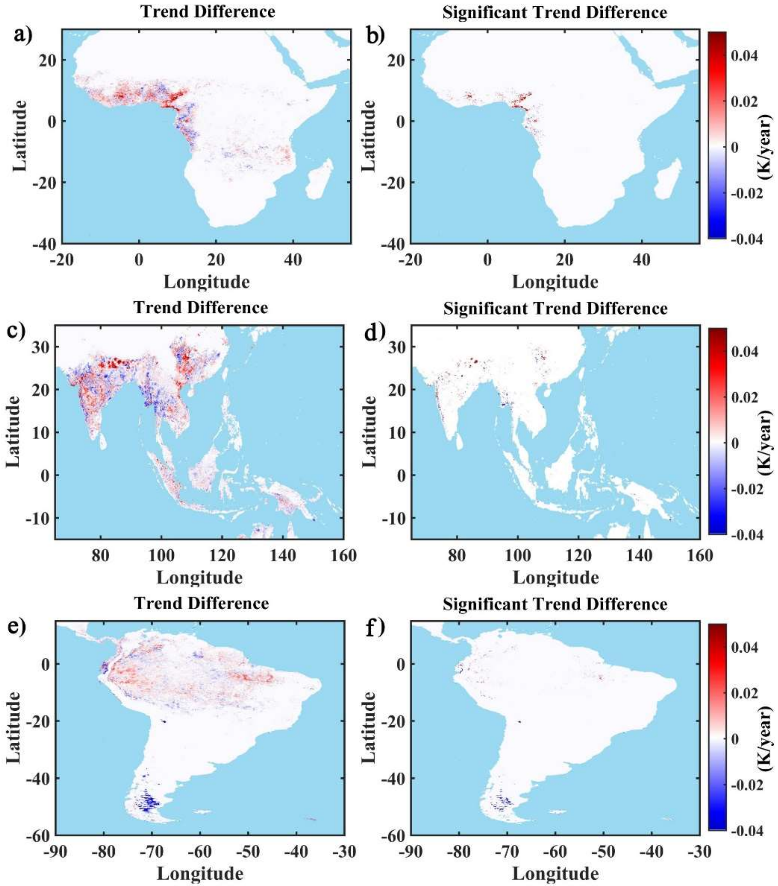
3.2. Trend Difference

For climate change analysis on geophysical observation data, substantial data gaps always present large spatial and temporal differences, which may reduce the usage rate and hinder subsequent interpretation by generating uncertainties in time series trend. An effective gap-filling method will be helpful in giving a solution to this impediment. Here we attempt to assess the trend differences between original LST and estimated LST on three continents to show the influence of gaps on the LST time series trend. According to the testing framework of temperature time series involving satellite radiosonde and reanalysis datasets [49,50], the OLS linear time series trends are estimated, and the trend differences are examined between two corresponding LST time series from January 2001 to December 2017 at each LST pixel on the gap region.

We note that there is a wide range of trend differences in LST after gaps filling process (Figure 6a,c,e). Although both the evaluation indicators and OLS linear fit results demonstrated the close correspondence between the original LST and the estimated LST in (Section 3.1), low and high biases (-0.04–0.04 K/year) in LST time series trends are presented, mainly distributed in data gaps. Referred to the distribution of actual time series trends, estimation uncertainties of the LST trend are presented due to substantial data gaps in original LST, with a relatively larger cooling or warming tendency in the estimated LST at part of the regions (Figure S3). With respect to the significance examination, significant trend differences at the 95% confidence level (Figure 6b,d,f) are also particularly present in regions with large missing counts, i.e., Nigeria, India, Myanmar, and Southern Argentina (Figure 1), which confirms the hazard of data gaps.

Moreover, as shown in Figure 6a,c,e, the low biases and high biases of trend differences do not present a certain spatial distribution pattern, which is consistent with the trend uncertainty in LST time series. Compared to regions without missing data, these trend differences mainly result from the substantial data gaps due to bad climatic conditions and frequent cloud cover. If these data gaps cannot be properly solved during data processing, it will obstruct the subsequent analysis of spatial patterns and temporal trends of LST at both local and global scales, and consequently cause unsoundness of agreement between MODIS LST and other LST datasets. It is also noted that the trend differences of LST time series with “random blanking” pixels (as shown in Figure 3b, Figure 4b, and Figure 5b) are not statistically significant (Figure 6b,d,f), which indicates that the time series trends are approximated well by the DCT-PLS method, and the estimated LSTs have a close agreement with the original LSTs. The study of the significant trend differences helps to reveal the statistical uncertainties that hamper the utilization of the MODIS LST datasets.

4. Discussion

4.1. Fast and Robust Filling

Although the previous literature on filling MODIS LST have produced complete and high-quality filling results, which are based on data fusion between different satellite products, an empirical model containing other environmental factors, and multi-step temporal or spatial interpolations [13,26,27,51,52,53]. However, these filling processes greatly depend on adding corresponding ancillary LST datasets or external environmental factors with high spatio-temporal resolution. In contrast, the DCT-PLS method utilizes the advantage of DCT on the reconstruction of evenly spaced data and controls the smoothness by PLS algorithm [46], benefiting the reconstruction independent from ancillary datasets, which makes the algorithm well adapted to the gap-filling purpose for long time series and large spatial coverage geophysical dataset.

Based on DCT and IDCT, the DCT-PLS method explicitly uses the integral spatial information of the LST dataset to derive a statistical model and fill data gaps. Rather than reducing the noise in LST, both high and low original LST values are retained when obtaining the optimal smoothing parameter. By preserving high frequency components of LST, information of spatial pattern and details are reconstructed simultaneously on gap region (Figure 3c, Figure 4c, Figure 5c for monthly LST and S4c, S4f, S4i for eight-day LST). The validation of entire filling results over full-time series show a strong correlation (R² of 0.98, 0.98, 0.98, and RMSE of 0.73 K, 0.9 K, 0.81 K for three continents) and a close agreement (absolute value biases of three continents are all less than 0.001 K) between estimated LST and original LST of both full-time series (Figure S2) and each layer (Figure S5). The results of MODIS eight-day LST (Figure S4 and Table S1) and MODIS daily LST [42] also indicate a good filling application.

Controlling by the smoothing parameter s, a high s value can lead to losses of high frequency components and the optimal s should be smaller than 0.5 to prevent over-smoothing effect for PIV data [47]. More data noise can be smoothed with a high value of s, but the details will be blurred with smoother filling results, while the minor fluctuations over data gaps may be exaggerated with an infinitesimal s value smaller than 10^-7 for filling of soil moisture [39]. Thus, a properly small smoothing parameter is required to preserve the information in original LST data and fill gaps. Defining a minimum global average reconstruction error, Wang et al. suggested 10⁻⁶ for filling gaps in both daytime and nighttime soil moisture datasets at the global scale [39]. Figure S6 presents the variation of global average reconstruction error and smoothing parameter s for each iteration of DCT-PLS filling process over full LST time series. As shown, filling processes of three regions converge to smoothing parameters of 7 × 10^-3, 9 × 10^-3, and 10^-2 respectively, which implies the selection of smoothing parameter may vary with different climate conditions, heterogeneous landscapes, and different retrievals. Pham et al. suggested applying different smoothing parameters for filling gaps of daily LST in Australia, in which s is smaller than or equal to 10⁻⁶ for daytime products and s ≤ 10^-4 for nighttime products [42]. However, optimized by the GCV score criterion, the automatically determined smoothing parameters benefit the DCT-PLS, applying varying filling processes and achieving a small reconstruction error without losing both high and low-frequency components of datasets.

As previously mentioned, the DCT-PLS has some novel features with respect to other gap-filling methods. Using both spatial and temporal information of the dataset to derive the statistical model and fill gaps, the DCT-PLS method is well adapted to fill substantial gaps in large spatio-temporal geophysical datasets. Computing the most appropriate smoothing parameter s in each iteration helps to avoid both over- and under-smoothing effect and eliminates the need for complicated parameterizations to obtain an accurate filling result. Compared with sophisticated geostatistical approaches involving additional coding efforts and processing time [54], the DCT-PLS method owns a fast and robust computation process with the automatic parameter optimization algorithm. Meanwhile, independent of any ancillary datasets, including other LST observations or external environmental factors, this method avoids additional uncertainty. In general, it demonstrates that the DCT-PLS method owns the advantages of large spatial filling coverage, high reconstruction accuracy, and independent and fast processing.

4.2. Gap Impediment

To assess whether the availability of LST is improved after gaps filling process and examine the uncertainties of the LST time series trend caused by data gaps, trend differences are computed over a full-time series. The results show that time series trends have a significant discrepancy ranging in -0.04-0.04 K/year. The distribution of low biases and high biases do not show apparent spatial pattern (Figure 6a,c,e), and the filling results indicate different trend difference on either cooling or warming region (Figure S3), which indicates that trend differences of time series in LST caused by data gaps are uncertain in space. Shown in the significance examination results (Figure 6b, 6d, and 6f), the Gulf of Guinea coast, west coast of India, southern Myanmar, western Ecuador, and the amazon estuary area show apparent trend differences at the 95% confidence level, where have large missing counts in time series (Figure 1). This could demonstrate the non-negligible influences on the LST time series trend due to data gaps [55].

Moreover, we also find that although the Indonesian islands have large missing counts, trend differences are not statistically significant in that region. This can be attributed to the fact that gaps generated in this area are probably not the extreme values in time series, which can be well reconstructed by DCT-PLS and have no significant impact on time series trends. In contrast, although there are no large missing counts in southern China, data gaps in this region also produce significant trend differences. Compared to the seasonal gaps affected by the monsoon climate, the gaps in southern China may be suffered from local terrain effects or other local variable atmospheric disturbances [56]. In addition, the large areas of significant trend difference in Patagonia and Himalayas imply the impact of elevation on LST reconstruction. As closely LST-related factors [11,57], the topography is complex and the elevation in these regions is above 3,000 m, which lead to hampers towards the MODIS LST reconstruction. Thus, obtaining realistic LST in these regions will depend on high-quality external ancillary data as predictors to enhance the spatial details [25]. Similarly, ancillary information is also needed for filling the gaps with large continuous missing areas to generate accurate surfaces (Figure S7), which is consistent with the result obtained by Pham et al. [42]. With respect to small continuous gap area or discrete gaps, generally produced by cloud cover, aerosol, and difficult atmospheric conditions instead of sensor malfunctioning or satellite scanning gaps [58], the DCT-PLS method have a good filling skill of MODIS LST gaps (Figure S7).

In general, although performance of DCT-PLS method is restricted in some heterogeneous regions or local complex terrain, and the filling accuracy decreases with large gap areas, the overall low bias and visually acceptable filling results demonstrate that this method is applicable to fill gaps of large spatio-temporal MODIS LST datasets on global scale over different land covers and climate conditions. However, for regions with complex terrain details or large continuous gaps, the feasibility of the DCT-PLS method is worthy of further exploration. Available ancillary information may benefit obtaining accurate local surfaces.

5. Conclusions

Common interpolation methods of filling data gaps in MODIS LST datasets are performed at local spatial coverage; For large spatial coverage, high spatio-temporal resolution ancillary datasets are necessary to provide more spatial details for the filling process. To solve this problem, we have presented and discussed the DCT-PLS method to reconstruct MODIS LST datasets. It is based on penalized least squares and discrete cosine transform, plus the GCV criterion for the optimal choice of the smoothing parameter. This approach can complete the filling process just on MODIS LST data without requiring other ancillary information. In addition, because of the lower computational complexity of DCT and IDCT, evenly spaced data like MODIS LST can be easily filled. More importantly, robust smoothing performs well on all values, including extreme values. By reconstructing the high frequency components, this method retains the global spatial patterns of the original LST.

The gaps filling process is performed on MODIS LST at a global scale. To assess the feasibility of DCT-PLS method, evaluation indicators are computed on simulated gaps for each continent. As demonstrated by our results, although the DCT-PLS method is affected by fragmental regions and a wide range of original LST values, the filling results explicitly present globally close agreements between estimated LST and original LST with 0.95 average R², 0.91K average RMSE, and 0.01K average bias. Further, by estimating trend differences in LST time series, significant trend differences are revealed at regions with large missing counts, which indicates that substantial data gaps could cause obvious trend uncertainties with over- and under-estimation. With respect to the significance examination, the necessity of gaps filling in MODIS LST and the availability of DCT-PLS filling method are confirmed conclusively.

In summary, it is practical to use the fast and robust DCT-PLS method to fill data gaps of monthly MODIS daytime LST datasets and reconstruct the integral spatial patterns and subtle spatial details at a global scale. However, for filling process at a local spatial coverage or regions with complex terrain, the extreme values in the fluctuant series might be over- and under-estimated by integral smoothing or partial overfitting. That may generate uncertainties in trend patterns. Therefore, we suggest further study on the validation of DCT-PLS method at local scale of MODIS LST datasets or other large geophysical datasets. The Matlab code for the DCT-PLS method is available from http://www.biomecardio.com/matlab/smoothn.html.

References

1. Hall, A.; Louis, J.; Lamb, D. Characterising and mapping vineyard canopy using high-spatial-resolution aerial multispectral images. Comput. Geosci. 2003, 29, 813–822. [Google Scholar] [CrossRef]
2. Arno, J.; Martinez-Casasnovas, J.A.; Ribes-Dasi, M.; Rosell, J.R. Review. Precision Viticulture. Research topics, challenges and opportunities in site-specific vineyard management. Span. J. Agric. Res. 2009, 7, 779–790. [Google Scholar] [CrossRef] [Green Version]
3. Mannstein, H. Surface Energy Budget, Surface Temperature and Thermal Inertia. In Remote Sensing Applications in Meteorology and Climatology; Vaughan, R.A., Ed.; Springer: Dordrecht, The Netherlands, 1987; pp. 391–410. [Google Scholar] [CrossRef]
4. Sellers, P.J.; Hall, F.G.; Asrar, G.; Strebel, D.E.; Murphy, R.E. THE 1ST ISLSCP FIELD EXPERIMENT (FIFE). Bull. Am. Meteorol. Soc. 1988, 69, 22–27. [Google Scholar] [CrossRef] [Green Version]
5. Hu, L.Q.; Brunsell, N.A.; Monaghan, A.J.; Barlage, M.; Wilhelmi, O.V. How can we use MODIS land surface temperature to validate long-term urban model simulations? J. Geophys. Res. Atmos. 2014, 119, 3185–3201. [Google Scholar] [CrossRef] [Green Version]
6. Chen, S.S.; Chen, X.Z.; Chen, W.Q.; Su, Y.X.; Li, D. A simple retrieval method of land surface temperature from AMSR-E passive microwave data-A case study over Southern China during the strong snow disaster of 2008. Int. J. Appl. Earth Obs. Geoinf. 2011, 13, 140–151. [Google Scholar] [CrossRef]
7. Bisht, G.; Venturini, V.; Islam, S.; Jiang, L. Estimation of the net radiation using MODIS (Moderate Resolution Imaging Spectroradiometer) data for clear sky days. Remote Sens. Environ. 2005, 97, 52–67. [Google Scholar] [CrossRef]
8. Batra, N.; Islam, S.; Venturini, V.; Bisht, G.; Jiang, L. Estimation and comparison of evapotranspiration from MODIS and AVHRR sensors for clear sky days over the Southern Great Plains. Remote Sens. Environ. 2006, 103, 1–15. [Google Scholar] [CrossRef]
9. Hengl, T.; Heuvelink, G.B.M.; Tadic, M.P.; Pebesma, E.J. Spatio-temporal prediction of daily temperatures using time-series of MODIS LST images. Theor. Appl. Climatol. 2012, 107, 265–277. [Google Scholar] [CrossRef] [Green Version]
10. Kilibarda, M.; Hengl, T.; Heuvelink, G.B.; Gräler, B.; Pebesma, E.; Perčec Tadić, M.; Bajat, B. Spatio-temporal interpolation of daily temperatures for global land areas at 1 km resolution. J. Geophys. Res. Atmos. 2014, 119, 2294–2313. [Google Scholar] [CrossRef] [Green Version]
11. Neteler, M. Estimating Daily Land Surface Temperatures in Mountainous Environments by Reconstructed MODIS LST Data. Remote Sens. 2010, 2, 333–351. [Google Scholar] [CrossRef] [Green Version]
12. Yu, W.; Tan, J.; Ma, M.; Li, X.; She, X.; Song, Z. An Effective Similar-Pixel Reconstruction of the High-Frequency Cloud-Covered Areas of Southwest China. Remote Sens. 2019, 11, 336. [Google Scholar] [CrossRef] [Green Version]
13. Crosson, W.L.; Al-Hamdan, M.Z.; Hemmings, S.N.J.; Wade, G.M. A daily merged MODIS Aqua-Terra land surface temperature data set for the conterminous United States. Remote Sens. Environ. 2012, 119, 315–324. [Google Scholar] [CrossRef]
14. Zeng, C.; Shen, H.F.; Zhong, M.L.; Zhang, L.P.; Wu, P.H. Reconstructing MODIS LST Based on Multitemporal Classification and Robust Regression. IEEE Geosci. Remote Sens. Lett. 2015, 12, 512–516. [Google Scholar] [CrossRef]
15. Kang, J.; Tan, J.; Jin, R.; Li, X.; Zhang, Y. Reconstruction of MODIS land surface temperature products based on multi-temporal information. Remote Sens. 2018, 10, 1112. [Google Scholar] [CrossRef] [Green Version]
16. Scharlemann, J.P.; Benz, D.; Hay, S.I.; Purse, B.V.; Tatem, A.J.; Wint, G.W.; Rogers, D.J. Global data for ecology and epidemiology: A novel algorithm for temporal Fourier processing MODIS data. PLoS ONE 2008, 3, e1408. [Google Scholar] [CrossRef]
17. Li, X.; Shen, H.; Zhang, L.; Zhang, H.; Yuan, Q.; Yang, G. Recovering quantitative remote sensing products contaminated by thick clouds and shadows using multitemporal dictionary learning. IEEE Trans. Geosci. Remote Sens. 2014, 52, 7086–7098. [Google Scholar]
18. Masiello, G.; Serio, C.; De Feis, I.; Amoroso, M.; Venafra, S.; Trigo, I.F.; Watts, P. Kalman filter physical retrieval of surface emissivity and temperature from geostationary infrared radiances. Atmos. Meas. Tech. 2013, 6, 3613–3634. [Google Scholar] [CrossRef] [Green Version]
19. Blasi, M.; Liuzzi, G.; Masiello, G.; Serio, C.; Telesca, V.; Venafra, S.J.T. Surface parameters from seviri observations through a kalman filter approach: Application and evaluation of the scheme to the southern Italy. Tethys 2016, 13, 1–19. [Google Scholar] [CrossRef]
20. Liu, Z.; Wu, P.; Duan, S.; Zhan, W.; Ma, X.; Wu, Y. Spatiotemporal reconstruction of land surface temperature derived from fengyun geostationary satellite data. IEEE J. Sel. Top. Appl. Earth Obs. Remote Sens. 2017, 10, 4531–4543. [Google Scholar] [CrossRef]
21. Shen, H.; Li, X.; Cheng, Q.; Zeng, C.; Yang, G.; Li, H.; Zhang, L. Missing information reconstruction of remote sensing data: A technical review. IEEE Geosci. Remote Sens. Mag. 2015, 3, 61–85. [Google Scholar] [CrossRef]
22. Kou, X.K.; Jiang, L.M.; Bo, Y.C.; Yan, S.; Chai, L.N. Estimation of Land Surface Temperature through Blending MODIS and AMSR-E Data with the Bayesian Maximum Entropy Method. Remote Sens. 2016, 8, 17. [Google Scholar] [CrossRef] [Green Version]
23. Xu, S.; Cheng, J.; Zhang, Q. Reconstructing All-Weather Land Surface Temperature Using the Bayesian Maximum Entropy Method Over the Tibetan Plateau and Heihe River Basin. IEEE J. Sel. Top. Appl. Earth Obs. Remote Sens. 2019, 12, 3307–3316. [Google Scholar] [CrossRef]
24. Zhang, X.; Zhou, J.; Göttsche, F.-M.; Zhan, W.; Liu, S.; Cao, R. A Method Based on Temporal Component Decomposition for Estimating 1-km All-Weather Land Surface Temperature by Merging Satellite Thermal Infrared and Passive Microwave Observations. IEEE Trans. Geosci. Remote Sens. 2019, 57, 4670–4691. [Google Scholar] [CrossRef]
25. Metz, M.; Rocchini, D.; Neteler, M. Surface Temperatures at the Continental Scale: Tracking Changes with Remote Sensing at Unprecedented Detail. Remote Sens. 2014, 6, 3822–3840. [Google Scholar] [CrossRef] [Green Version]
26. Sun, L.; Chen, Z.; Gao, F.; Anderson, M.; Song, L.; Wang, L.; Hu, B.; Yang, Y. Reconstructing daily clear-sky land surface temperature for cloudy regions from MODIS data. Comput. Geosci. 2017, 105, 10–20. [Google Scholar] [CrossRef]
27. Duan, S.B.; Li, Z.L.; Leng, P. A framework for the retrieval of all-weather land surface temperature at a high spatial resolution from polar-orbiting thermal infrared and passive microwave data. Remote Sens. Environ. 2017, 195, 107–117. [Google Scholar] [CrossRef]
28. Weiss, D.J.; Atkinson, P.M.; Bhatt, S.; Mappin, B.; Hay, S.I.; Gething, P.W. An effective approach for gap-filling continental scale remotely sensed time-series. ISPRS J. Photogramm. Remote Sens. 2014, 98, 106–118. [Google Scholar] [CrossRef] [Green Version]
29. Metz, M.; Andreo, V.; Neteler, M. A New Fully Gap-Free Time Series of Land Surface Temperature from MODIS LST Data. Remote Sens. 2017, 9, 19. [Google Scholar] [CrossRef] [Green Version]
30. Yang, G.; Sun, W.; Shen, H.; Meng, X.; Li, J. An Integrated Method for Reconstructing Daily MODIS Land Surface Temperature Data. IEEE J. Sel. Top. Appl. Earth Obs. Remote Sens. 2019, 12, 1026–1040. [Google Scholar] [CrossRef]
31. Sarhan, A.M. Cancer classification based on microarray gene expression data using DCT and ANN. J. Theor. Appl. Inf. Technol. 2009, 6, 208–216. [Google Scholar]
32. Rawat, C.S.; Meher, S. A Hybrid Image Compression Scheme using DCT and Fractal Image Compression. Int. Arab J. Inf. Technol. 2013, 10, 553–562. [Google Scholar]
33. Vig, R.; Chauhan, S.S. Speech Compression using Multi-Resolution Hybrid Wavelet using DCT and Walsh Transforms. Procedia Comput. Sci. 2018, 132, 1404–1411. [Google Scholar] [CrossRef]
34. Amato, U.; De Feis, I. Smoothing data with correlated noise via Fourier transform. Math. Comput. Simul. 2000, 52, 175–196. [Google Scholar] [CrossRef]
35. Ahmed, N.; Natarajan, T.; Rao, K.R. Discrete Cosine Transform. IEEE Trans. Comput. C 1974, 23, 90–93. [Google Scholar] [CrossRef]
36. Amato, U.; De Feis, I. Convergence for the regularized inversion of Fourier series. J. Comput. Appl. Math. 1997, 87, 261–284. [Google Scholar] [CrossRef] [Green Version]
37. Liu, Z.; Li, Y.; Sun, F.; He, J.; Qi, C.; Luo, D. A Robust Recoverable Algorithm Used for Digital Speech Forensics Based on DCT; Springer International Publishing: Cham, Switzerland, 2018. [Google Scholar]
38. Sunu, C.; Toker, C. Sparse 2D-DCT Reconstruction of Total Electron Content Maps. In Proceedings of the 2019 9th International Conference on Recent Advances in Space Technologies (RAST), Istanbul, Turkey, 11–14 June 2019; pp. 667–672. [Google Scholar]
39. Wang, G.J.; Garcia, D.; Liu, Y.; de Jeu, R.; Dolman, A.J. A three-dimensional gap filling method for large geophysical datasets: Application to global satellite soil moisture observations. Environ. Model. Softw. 2012, 30, 139–142. [Google Scholar] [CrossRef]
40. Kim, S.; Paik, K.; Johnson, F.M.; Sharma, A. Building a flood-warning framework for ungauged locations using low resolution, open-access remotely sensed surface soil moisture, precipitation, soil, and topographic information. IEEE J. Sel. Top. Appl. Earth Obs. Remote Sens. 2018, 11, 375–387. [Google Scholar] [CrossRef]
41. Lei, F.N.; Crow, W.T.; Shen, H.F.; Su, C.H.; Holmes, T.R.H.; Parinussa, R.M.; Wang, G.J. Assessment of the impact of spatial heterogeneity on microwave satellite soil moisture periodic error. Remote Sens. Environ. 2018, 205, 85–99. [Google Scholar] [CrossRef]
42. Pham, H.T.; Kim, S.; Marshall, L.; Johnson, F. Using 3D robust smoothing to fill land surface temperature gaps at the continental scale. Int. J. Appl. Earth Obs. Geoinf. 2019, 82, 6. [Google Scholar] [CrossRef]
43. Wan, Z.M.; Dozier, J. A generalized split-window algorithm for retrieving land-surface temperature from space. IEEE Trans. Geosci. Remote Sens. 1996, 34, 892–905. [Google Scholar]
44. MOD11A2 MODIS/Terra land surface temperature/emissivity 8 day L3 global 1km SIN grid V006. Available online: https://lpdaac.usgs.gov/products/mod11a2v006/ (accessed on 1 October 2019).
45. Wan, Z.M. New refinements and validation of the MODIS Land-Surface Temperature/Emissivity products. Remote Sens. Environ. 2008, 112, 59–74. [Google Scholar] [CrossRef]
46. Garcia, D. Robust smoothing of gridded data in one and higher dimensions with missing values. Comput. Stat. Data Anal. 2010, 54, 1167–1178. [Google Scholar] [CrossRef] [Green Version]
47. Garcia, D. A fast all-in-one method for automated post-processing of PIV data. Exp. Fluids 2010, 50, 1247–1259. [Google Scholar] [CrossRef] [PubMed]
48. Craven, P.; Wahba, G. Smoothing Noisy Data with Spline Functions-Estimating the Correct Degree of Smoothing by the Method of Generalized Cross-Validation. Numer. Math. 1978, 31, 377–403. [Google Scholar] [CrossRef]
49. Santer, B.D.; Hnilo, J.J.; Wigley, T.M.L.; Boyle, J.S.; Doutriaux, C.; Fiorino, M.; Parker, D.E.; Taylor, K.E. Uncertainties in observationally based estimates of temperature change in the free atmosphere. J. Geophys. Res. Atmos. 1999, 104, 6305–6333. [Google Scholar] [CrossRef]
50. Santer, B.D.; Wigley, T.M.L.; Boyle, J.S.; Gaffen, D.J.; Hnilo, J.J.; Nychka, D.; Parker, D.E.; Taylor, K.E. Statistical significance of trends and trend differences in layer-average atmospheric temperature time series. J. Geophys. Res. Atmos. 2000, 105, 7337–7356. [Google Scholar] [CrossRef]
51. Xu, Y.M.; Shen, Y. Reconstruction of the land surface temperature time series using harmonic analysis. Comput. Geosci. 2013, 61, 126–132. [Google Scholar] [CrossRef]
52. Weng, Q.; Fu, P.; Gao, F. Generating daily land surface temperature at Landsat resolution by fusing Landsat and MODIS data. Remote Sens. Environ. 2014, 145, 55–67. [Google Scholar] [CrossRef]
53. Li, X.; Zhou, Y.; Asrar, G.R.; Zhu, Z. Creating a seamless 1 km resolution daily land surface temperature dataset for urban and surrounding areas in the conterminous United States. Remote Sens. Environ. 2018, 206, 84–97. [Google Scholar] [CrossRef]
54. Lloyd, C.D.; Atkinson, P.M. Deriving DSMs from LiDAR data with kriging. Int. J. Remote Sens. 2002, 23, 2519–2524. [Google Scholar] [CrossRef]
55. Westermann, S.; Langer, M.; Ostby, T.; Boike, J.; Schuler, T.; Etzelmuller, B. In-situ validation of remotely sensed land surface temperatures in high-arctic land regions-implications for gap filling and trend analyses. In Proceedings of the AGU Fall Meeting, San Francisco, CA, USA, 14 December 2015. [Google Scholar]
56. Liu, Y.; Noumi, Y.; Yamaguchi, Y.J.S. Discrepancy between ASTER-and MODIS-derived land surface temperatures: Terrain effects. Sensors 2009, 9, 1054–1066. [Google Scholar] [CrossRef] [PubMed]
57. Linghong, K.E.; Zhengxing, W.; Chunqiao, S.; Zhenquan, L.U. Reconstruction of MODIS LST Time Series and Comparison with Land Surface Temperature (T) among Observation Stations in the Northeast Qinghai-Tibet Plateau. Prog. Geogr. 2011, 30, 819–826. [Google Scholar]
58. Ghafarian Malamiri, H.R.; Rousta, I.; Olafsson, H.; Zare, H.; Zhang, H. Gap-Filling of MODIS Time Series Land Surface Temperature (LST) Products Using Singular Spectrum Analysis (SSA). Atmosphere 2018, 9, 18. [Google Scholar] [CrossRef] [Green Version]
Figure 1. Number of missing values for the monthly MODIS daytime LST from 2001–2017.
Remotesensing 12 00361 g001
Figure 2. Flowchart of filling monthly MODIS daytime LST gaps. The experimental procedures are indicated by the shaded roman numerals (I–V). Gray blocks in this flowchart represent non-empty LST pixels, white blocks with full borders represent the original gaps and white blocks with dotted borders represent the simulated gaps. The detailed descriptions are given at the end of Section 2.3 with five paragraphs, which are corresponding with numerals I–V.
Remotesensing 12 00361 g002
Figure 3. DCT-PLS filling results of Africa LST: (a) distribution of original missing value; (b) distribution of simulated missing value (red pixels) covers the original missing value (dark blue pixels); (c) estimated LST data; (d) evaluation of estimated LST based on DCT-PLS against the original LST.
Remotesensing 12 00361 g003
Figure 4. DCT-PLS filling results of Southeast Asia LST: (a) distribution of original missing value; (b) distribution of simulated missing value (red pixels) covers the original missing value (dark blue pixels); (c) estimated LST data; (d) evaluation of estimated LST based on DCT-PLS against the original LST.
Remotesensing 12 00361 g004
Figure 5. DCT-PLS filling results of South America LST: (a) distribution of original missing value; (b) distribution of simulated missing value (red pixels) covers the original missing value (dark blue pixels); (c) estimated LST data; (d) evaluation of estimated LST based on DCT-PLS against the original LST.
Remotesensing 12 00361 g005
Figure 6. Trend differences between the original LST and estimated LST: (a, c, e) trend differences of LST in Africa, Southeast Asia, and South America, respectively; (b, d, f) significance of trend differences in Africa, Southeast Asia, and South America, respectively.
Remotesensing 12 00361 g006