Article

FGATR-Net: Automatic Network Architecture Design for Fine-Grained Aircraft Type Recognition in Remote Sensing Images

1
Aerospace Information Research Institute, Chinese Academy of Sciences, Beijing 100190, China
2
Key Laboratory of Network Information System Technology (NIST), Aerospace Information Research Institute, Chinese Academy of Sciences, Beijing 100190, China
3
University of Chinese Academy of Sciences, Beijing 100190, China
4
School of Electronic, Electrical and Communication Engineering, University of Chinese Academy of Sciences, Beijing 100190, China
*
Author to whom correspondence should be addressed.
These authors contributed equally to this work.
Remote Sens. 2020, 12(24), 4187; https://doi.org/10.3390/rs12244187
Submission received: 25 November 2020 / Revised: 14 December 2020 / Accepted: 17 December 2020 / Published: 21 December 2020

Abstract

:
Fine-grained aircraft type recognition in remote sensing images, aiming to distinguish different types of the same parent category aircraft, is quite a significant task. In recent decades, with the development of deep learning, the solution scheme for this problem has shifted from handcrafted feature design to model architecture design. Although a great progress has been achieved, this paradigm generally needs strong expert knowledge and rich expert experience. It is still an extremely laborious work and the automation level is relatively low. In this paper, inspired by Neural Architecture Search (NAS), we explore a novel differentiable automatic architecture design framework for fine-grained aircraft type recognition in remote sensing images. In our framework, the search process is divided into several phases. Network architecture deepens at each phase while the number of candidate functions gradually decreases. To achieve it, we adopt different pruning strategies. Then, the network architecture is determined through a potentiality judgment after an architecture heating process. This approach can not only search deeper network, but also reduce the computational complexity, especially for relatively large size of remote sensing images. When all differentiable search phases are finished, the searched model called Fine-Grained Aircraft Type Recognition Net (FGATR-Net) is obtained. Compared with previous NAS, ours are more suitable for relatively large and complex remote sensing images. Experiments on Multitype Aircraft Remote Sensing Images (MTARSI) and Aircraft17 validate that FGATR-Net possesses a strong capability of feature extraction and feature representation. Besides, it is also compact enough, i.e., parameter quantity is relatively small. This powerfully indicates the feasibility and effectiveness of the proposed automatic network architecture design method.

1. Introduction

With the great progress of remote sensing imaging, there are significant improvements for remote sensing images both in quantity and quality, which effectively propels the development of remote sensing interpretation. Aircraft type recognition, aiming to distinguish different types of aircraft, is a very important task in remote sensing field. It has profound significance not only for civil [1] but also in military [2], such as the airport scheduling, reconnaissance analysis, etc.. Consequently, it receives extensive attention of large number of researchers.
Different from general image classification, aircraft type recognition is a Fine-Grained Visual Classification (FGVC) task. Categories to be recognized are all subject to the same parent category. Hence, the interclass variance is relatively small, for all subcategories are quite similar in terms of appearance, behavior and so on. Besides, the intraclass is relatively large, being affected by the complexity of remote sensing image background, the diversity of temporal, the scene illumination changes, solar radiation angle, etc.. Therefore, aircraft type recognition in remote sensing images is still a very challenging problem.
In recent decades, a variety of effective methods have been proposed to solve fine-grained aircraft type recognition task in remote sensing images. Hsieh et al. [3] first extract bitmap, wavelet transform, Zernike moment and distance transform features and then leverage a novel weight learning algorithm to integrate these features. This method improves the recognition rate while it also achieves a higher robustness. Xu et al. [4] leverage Edge Potential Function (EPF) to obtain a best matching contour. Meantime, Artificial Bee Colony (ABC) algorithm that can avoid falling into local optimum is proposed to optimize EPF. Both theoretical and experimental analysis demonstrate the effectiveness of this method. Liu et al. [5] introduce a coarse-to-fine algorithm to recognize different aircraft types. Coarse stage roughly estimates the pose of aircraft in remote sensing images and the role of fine stage is to segment and recognize the type. Based on the cooperation of these two stages, there are improvements in series of experiments. Although plenty of good results have been achieved, these handcrafted feature design methods still face the problem of weak expression capability, poor generalization capability, etc..
With AlexNet [6], VGGNet [7], GoogLeNet [8] and a series of neural networks [9,10,11] proposed, deep learning methods have also been introduced into fine-grained aircraft type recognition task in remote sensing images. To tackle the problem of small interclass variance and large intraclass dissimilarity, Diao et al. [12] apply Deep Belief Net (DBN) [13] which consists of many Restricted Boltzmann Machines (RBMs) to realize recognition. This method reaches a higher level in speed and accuracy performance. Fu et al. [14] propose Multiple Class Activation Mapping (MultiCAM), including target net and object net, to fully utilize discriminative features. Besides, in view of relatively fewer remote sensing aircraft images, which has a negative impact on the training of deep learning methods, a novel framework is presented in [15]. This approach can cleverly transform aircraft type recognition into landmark detection. It helps to alleviate the dependence on labeled data. Experimental results show that the error rate can be reduced four fifths by using this method. And Zhang et al. [16] deal with this problem on the basis of conditional generative adversarial network [17] which can learn representative features without aircraft type labels. Generally, under the effect of deep learning, the paradigm has shifted from feature design to architecture design. However, there are also some shortcomings for deep learning methods. This design pattern usually needs strong expert knowledge and rich expert experience, especially for remote sensing field. Even so, a series of trial and error is also unavoidable and it is even an extremely laborious task. The automation and intellective level are still relatively low.
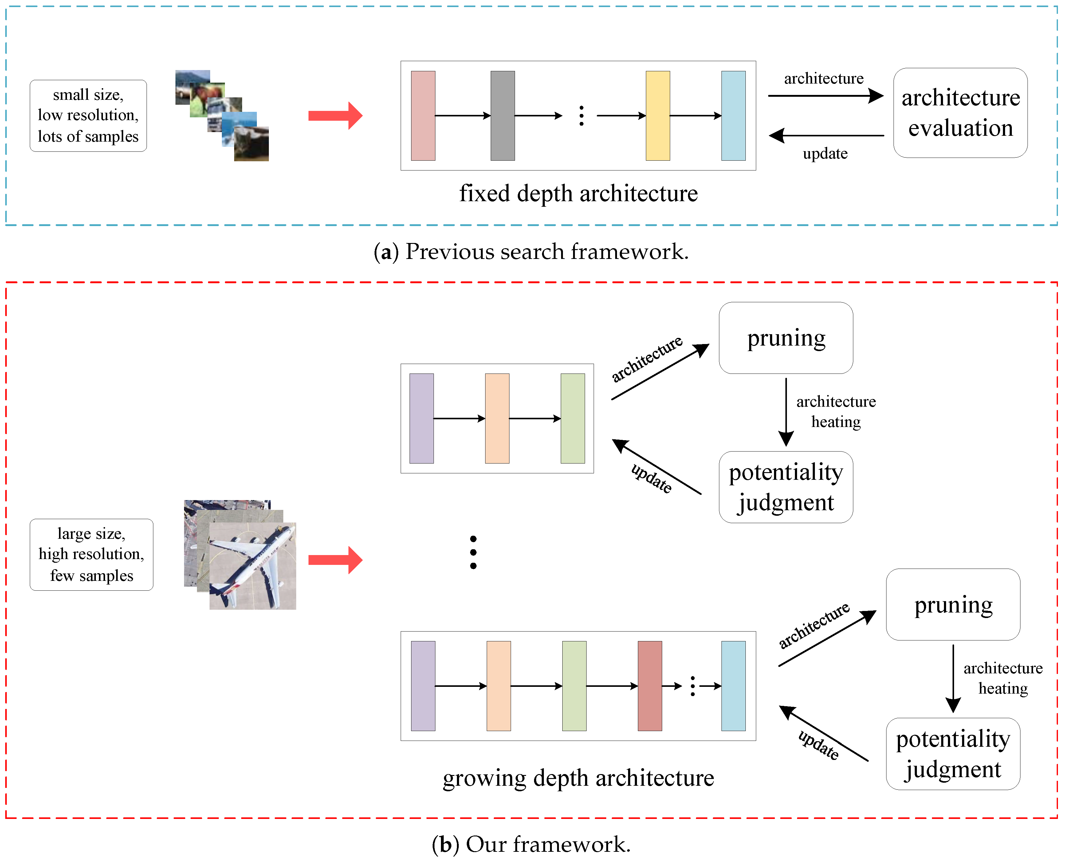
Recently, a novel framework named Neural Architecture Search (NAS) [18,19,20,21,22,23] is proposed to automatically design a neural network architecture. In NAS framework, complex architecture engineering can be greatly reduced. Hence, it has immediately attracted wide publicity and gradually becomes a research focus. An illustration of manual and automatic architecture design can be seen in Figure 1. In general, NAS can be divided into three classes according to the search strategy: Reinforcement Learning (RL) [18,19], Evolutionary Algorithm (EA) [20,21] and Gradient-Based method [22,23]. RL strategy takes a Long Short Term Memory (LSTM) [24] controller as an agent which can sample a network architecture in predefined search space by a certain probability. After that, the network is trained and the performance of it services as reward to optimize the controller by leveraging Policy Gradient. As for EA approach, a neural network architecture is regarded as a genotype. The optimization process is similar to natural selection in Biology field. Genotypes with poor performance are eliminated immediately while that performing well are retained. And then crossover and mutation are conducted among them. Different from RL and EA which both adopt discrete optimization procedure, Gradient-Based method utilizes a novel relaxation programme to transform search space to be continuous. By means of this technique, architecture search process can become differentiable and gradient descent algorithm is able to be applied in it. Moreover, the computational consumption is relatively low compared with the former two search strategies. For these reasons, Gradient-Based method is becoming widely popular.
As for the application of NAS in remote sensing, some pioneers have already made some explorations. Chen et al. [25] leverage Gradient-Based method to deal with HyperSpectral Image (HSI) classification task. Zhang et al. [26] propose an efficient search method to achieve an automatic network design procedure in semantic segmentation for high-resolution remote sensing images, which transfers NAS to a more advanced visual task. In this paper, we first attempt a novel differentiable automatic network architecture construction framework to achieve another shift in terms of design pattern for fine-grained aircraft type recognition in remote sensing images. The difference between previous NAS framework in natural scene images and ours can be referenced in Figure 2. To be specific, we utilize a differentiable approach where architecture parameters and weight parameters are optimized by turns in the search process. Due to the relatively large size of remote sensing images ( 32 × 32 in CIFAR-10 [27] while 156 × 156 in Aircraft17 [14] and 256 × 256 in MTARSI [28]), we search the network architecture in a growing way to avoid CUDA out of memory trouble caused by direct search method. Meanwhile, we also utilize pruning to cut off some weak connections at each search phase. Then, potentiality judgment can decide the network architecture after an architecture heating process. When all the search phases are finished, Fine-Grained Aircraft Type Recognition Net (FGATR-Net) is obtained. Ultimately, we train the FGATR-Net on target dataset from scratch. This design procedure is automatic and it not heavily relies on expert knowledge and artificial experience. In addition, series of experiments show that FGATR-Net outperforms all baseline models on fine-grained aircraft type recognition task not only in accuracy but also in lightweight, especially in the comparison with well-behaved EfficientNet [29] which is obtained by search approach. This strongly indicates that the proposed framework is a feasible and effective method. In summary, the main contributions of this paper are listed as follows:
  • A differentiable automatic network architecture design paradigm for fine-grained recognition in remote sensing images is explored for the first attempt to the best of our knowledge.
  • Considering the relatively large size of remote sensing images, network architecture deepens gradually in the search process. In the meanwhile, some unimportant edges are removed through different pruning strategies with the increase of network layers, making the network more compact.
  • In order to discriminate which architecture has more potential, we adopt potentiality judgment to determine the network architecture after an architecture heating process.
  • Experimental results on two challenging fine-grained aircraft type recognition datasets show that FGATR-Net is able to achieve the highest accuracy with just much fewer parameters. This strongly confirms the feasibility and effectiveness of the proposed method.
The rest of this article is organized as follows. Section 2 describes the proposed automatic architecture design framework in detail. In Section 3, datasets, evaluation metrics and implementation details are stated. And the experimental results to demonstrate the feasibility and effectiveness of our method are provided in Section 4. Subsequently, we have a discussion about the proposed method in Section 5. Ultimately, conclusions are drawn in Section 6 and the plan for further work is also given in this section.

2. Methodology

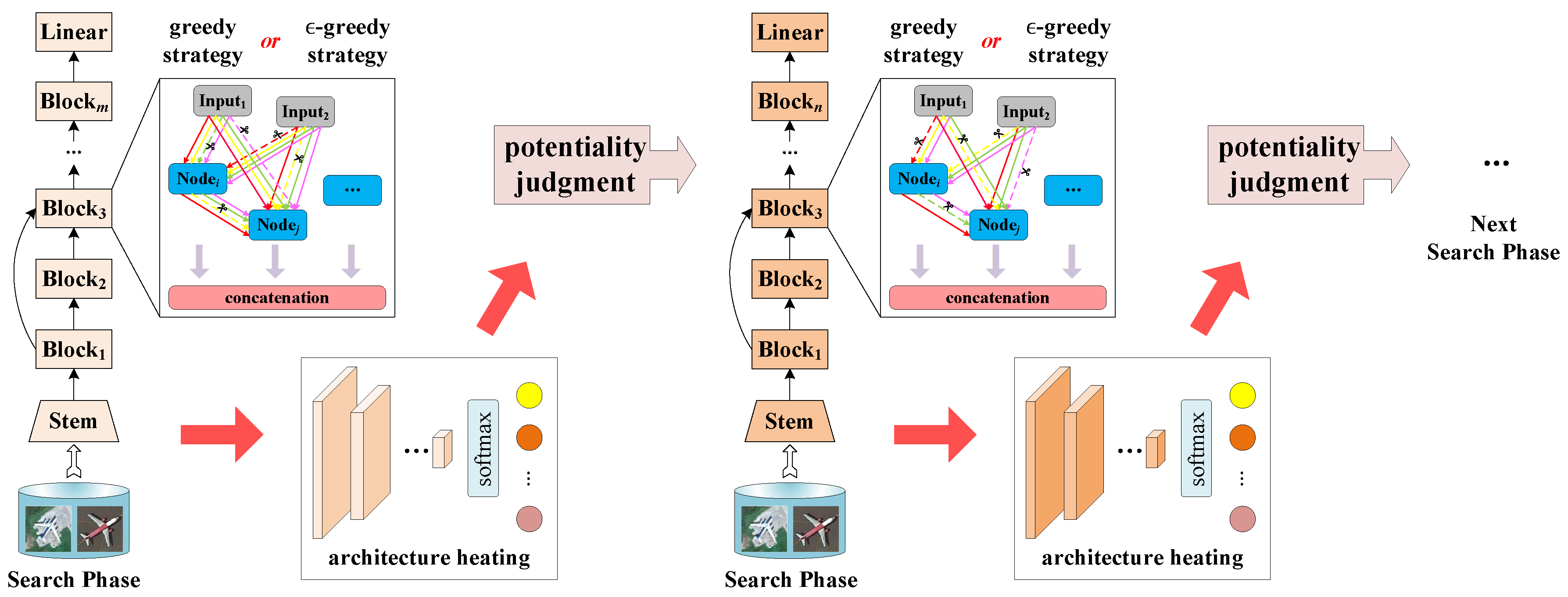
The overview of our search framework can be seen in Figure 3. The role of stem is to expand the number of channels and downsample the input remote sensing images. With the depth of the architecture growing gradually (Here, m < n ), some unimportant edges (indicated by dotted lines) will be pruned. Potentiality judgment can give a preliminary evaluation of two kinds of pruning strategies (i.e., greedy strategy and ϵ -greedy strategy). In the last search phase, we just adopt greedy strategy for there are only very few options. After getting the ultimate architecture, we can train it on the target dataset from scratch.

2.1. Differentiable Automatic Network Architecture Design

Popular Convolutional Neural Network (CNN) architecture generally contains many blocks which consist of some common components, such as convolution, pooling and so on. The component can be seen as a mathematical function f, where a feature map from one high dimensional space can be mapped into another. In NAS framework, we collect some candidate functions and organize them into a search space F . The purpose is to find out the optimal combination and connection relationship of these functions in a block. Then, these blocks are stacked layer by layer to construct the whole network. Different from RL-based [18,19] or EA-based [20,21] method, differentiable approach is more efficient and is easier to implement.

2.1.1. Block Representation as a DAG

We utilize a Directed Acyclic Graph (DAG) which is composed of M ordered nodes to represent a block. Each node in a block represents a feature map in high dimensional space. An edge of a DAG can be considered as a component in the search space. We first assume that each block has two different input nodes P 1 , P 2 and a single output node P M . Hence, there are M 3 middle nodes in total, that is { P i | 3 i M 1 , i N } . These two input nodes are taken from the output of two predecessor blocks. For middle node, it can be computed as:
P j = i < j f F [ f i s s e l e c t e d ] f ( P i )
where i , j separately represent the node index in DAG. [ · ] is Iverson bracket. If the expression inside the bracket is true, the bracket value is 1 and vice versa. The output node is the concatenation of all non-input nodes, which can be represented by:
P M = c o n c a t [ P 3 , P 4 , , P M 1 ]
where c o n c a t is the abbreviation of concatenation.

2.1.2. Architecture Parameters Relaxation

Components selection procedure is discrete, i.e., selected or discarded. Consequently, it is unable to be optimized by Back Propagation algorithm [30]. In order to make this process continuous, we apply softmax to all candidate functions between two nodes in DAG to relax the choice. This step can be described as:
α ˜ f ( i , j ) = e x p ( α f ( i , j ) ) f F e x p ( α f ( i , j ) )
o ˜ ( i , j ) = f F α ˜ f ( i , j ) f ( P i )
where α is architecture parameter which determines the importance of one component. o ˜ ( i , j ) is the weighted sum of all components from node i to node j. Through this approach, the architecture parameter can be transformed into [0, 1], making the optimization process feasible. When the architecture search is complete, the maximum architecture parameter between node i and node j can be obtained by:
α ˜ f ( i , j ) = a r g m a x f F ( α ˜ f ( i , j ) )
After that, to prevent excessive connections, the in-degree of node j is constrained to two. This means that only two most likely connections are preserved and the others are discarded.
The purpose of our method is to search for two types of blocks, namely, normal block and reduction block. For normal block, the stride of all components is 1 so that the size of feature map is maintained while the stride in reduction block is 2, enabling the searched model to downsample feature maps. Hence, the architecture parameters can be divided into 2 groups: α ˜ n o r m a l and α ˜ r e d u c t i o n . It is noteworthy that all normal blocks and all reduction blocks share the same α ˜ n o r m a l and α ˜ r e d u c t i o n respectively.

2.1.3. Optimization Policy

The optimization problem seems to be simpler after relaxation. However, it should not be ignored that architecture parameters α ˜ and weight parameters ω are coupled together. The loss function are determined by both α ˜ and ω . Aiming to decouple these two kinds of parameters, we leverage a bilevel optimization policy [31,32] to optimize them separately. Here, we use L t r a i n to denote training loss and L v a l is the validation loss. The optimization process can be expressed as:
m i n α ˜ L v a l ( ω , α ˜ )
s . t . ω = a r g m i n ω ( L t r a i n ( ω , α ˜ ) )
where ω represents the optimal weight parameter which is able to minimize the training loss. Through the alternate optimization, the best architecture parameter α ˜ and weight parameter ω can be obtained. Then the entire neural network can be constructed by decoding the best architecture parameter α ˜ . Next, the network can be trained from scratch as common measures [9,10].

2.2. Model Pruning Strategy

Although gradient decent algorithm is able to be applied with the aid of relaxation and bilevel optimization, the computational complexity is quite high for the weight parameters of all components need to be optimized simultaneously. The computational burden is not obvious in a dataset with relatively small size images such as CIFAR-10 [27] whose size is just 32 × 32 pixels. Nevertheless, for large size images especially for remote sensing images whose height and width commonly contain hundreds of pixels, the computation can be even unbearable. Therefore, we adopt a dynamic method to construct the whole network. As the network deepens, some components with poor performance will be excluded during the search phase. The specific growth process and pruning strategy are described below in detail.

2.2.1. Network Layers Growth

In general, network in the search process is relatively shallow compared with the ultimate architecture, due to the limitation of computation capability. However, according to some current studies [9,33,34], the depth of a network has a significant impact on its performance. The excellent architecture in search stage may perform poorly in evaluation stage.
Therefore, in order to improve the situation, we set the depth of network in the search stage to be equal to the ultimate architecture. However, considering the computational overhead, we adopt a gradual growth approach, rather than a direct one. Every time the network becomes deeper, some unimportant candidate functions in search space will be discarded through pruning. The pruning strategy will be stated in Section 2.2.2. This pattern not only offers the possibility of searching deeper architectures, but also relieves the computational burden brought by optimizing their architecture parameters and weight parameters.

2.2.2. Greedy Strategy and ϵ -Greedy Strategy

As regard to the pruning strategy, greedy pruning is a more basic method, which can be expressed by:
P P ( α ˜ f ( i , j ) ) = 1 , i f α ˜ f ( i , j ) = a r g m i n f F ( α ˜ f ( i , j ) ) 0 , i f α ˜ f ( i , j ) a r g m i n f F ( α ˜ f ( i , j ) )
where P P ( α ˜ f ( i , j ) ) is the pruning probability of component f between node i and node j. The pruned architecture can obtain the maximum reward under all known conditions by exploiting existing knowledge. Intuitively, this pruning strategy is also very reliable.
Nevertheless, greedy pruning strategy ignores the role of exploration to a certain degree. Typically, exploration and exploitation are two contradictory aspects when making decisions. The reward which the algorithm obtains will not grow, only exploiting existing knowledge. On the other hand, if just explore blindly, the risk will increase. This is exploration or exploitation dilemma [35]. Yet, ϵ -greedy strategy can alleviate this contradiction to a certain degree by setting a smaller ϵ . In this strategy, any candidate function may be pruned with the probability ϵ , otherwise remove the weakest edge. It can be written by:
P P ( α ˜ f ( i , j ) ) = ϵ | F | + 1 ϵ , i f α ˜ f ( i , j ) = a r g m i n f F ( α ˜ f ( i , j ) ) ϵ | F | , i f α ˜ f ( i , j ) a r g m i n f F ( α ˜ f ( i , j ) )
where | F | denotes the number of candidate functions in the predefined search space. It is also worth mentioning that the value of ϵ is not unchanged. It will gradually decrease as the pruning process proceeds. Theoretically, this jitter pruning approach can cover all candidate functions as far as possible, thus the exploration is more adequate on the basis of taking account of exploitation. Besides, it is easy to implement this strategy and no extra complex computation is brought.

2.2.3. Potentiality Judgment

In practice, when decision is not frequent, it is difficult to distinguish the behavior of the two strategies for both of them are local optimal methods. Meanwhile, we also can not examine its performance from a global perspective for the limitation of computation resources. Hence, in order to consider the stability of greedy strategy and the exploration of ϵ -greedy, we also add a simple validation before making the final decision. The original architecture is pruned by these two pruning strategies respectively after one search phase. We call them A g and A ϵ separately. Next, they are preliminarily trained for some epochs and evaluated on the validation set, called architecture heating. We take the best performance of the pruned architecture (i.e., recognition accuracy) as the evaluation metric of different pruning strategies. The final decision is based on the behavior of these two pruning strategies.
All in all, our search framework for FGATR-Net can be briefly summarized in Algorithm 1. After obtaining the final architecture A , we will train it from scratch as a common neural network. And then, it could converge on the target dataset through a sufficient training procedure.
Algorithm 1 Search framework for FGATR-Net.
Input: 
Initialized architecture parameters α and weight parameters ω ; Initialized architecture A 0 and search space F 0 ; Total search phases S P , search epochs E s e a r c h , training epochs E t r a i n ( E t r a i n < E s e a r c h ) and architecture heating epochs E h e a t i n g ; Training set D T ; Initialized ϵ and its decay coefficient t; Learning rate for weight parameters ξ A and for architecture parameters ξ B .
Output: 
Searched FGATR-Net.
1:
Divide D T into D A (updating weight parameters) and D B (updating architecture parameters).
2:
Initialization: A = A 0 , F = F 0 .
3:
while s p ∈ [1, S P ] do
4:
     for e p o c h ∈ [1, E s e a r c h ] do
5:
           Optimize weight parameters of A : ω ω ξ A ω L D A ( ω , α )
6:
           if e p o c h > E t r a i n then
7:
               Optimize architecture parameters of A : α α ξ B α L D B ( ω , α )
8:
           end if
9:
       end for
10:
       A g , F g ← greedy pruning strategy for A and F .
11:
       A ϵ , F ϵ ϵ -greedy pruning strategy for A and F with ϵ .
12:
     for i ∈ [1, E h e a t i n g ] do       // architecture heating process
13:
           P e r f o r m a n c e g ← optimize and evaluate A g .
14:
           P e r f o r m a n c e ϵ ← optimize and evaluate A ϵ .
15:
      end for
16:
      if P e r f o r m a n c e g P e r f o r m a n c e ϵ then
17:
           A = A ϵ and F = F ϵ .
18:
      else
19:
           A = A g and F = F g .
20:
      end if
21:
       ϵ = t ϵ .
22:
end while
23:
Obtain the searched FGATR-Net A .

3. Experiment Settings

3.1. Dataset

We conduct experiments on two challenging fine-grained aircraft type recognition datasets. The details of these two datasets are depicted as follow.

3.1.1. MTARSI

Multitype Aircraft Remote Sensing Images (MTARSI) [28] is a large-scale fine-grained aircraft type classification dataset. It is carefully annotated under the guidance of 7 experts in remote sensing interpretation. Thus, this dataset possesses a higher authority. In MTARSI, there are 9385 remote sensing images with different width and height extracted from Google Earth. The spatial resolution of these images changes from 1 m to 0.3 m. Totally, this dataset contains 20 types of aircraft and the quantity of images in each type of aircraft ranges from 230 to 846. Moreover, MTARSI has abundant multi temporal information. Images in MTARSI are selected at different times. It enriches the intraclass variation, bringing more difficulties to aircraft type recognition task. Besides, for each aircraft type, the models are quite different even though their appearances are similar. This makes one recognition algorithm difficult to distinguish different types, for the increasing of interclass similarity. Some aircraft examples of MTARSI are listed in Figure 4. As for the split of training set and test set, our approach is consistent with [28], that is four-fifths of the whole samples are selected for training and the rest are used for evaluation.

3.1.2. Aircraft17

Aircraft17 [14] is a challenging fine-grained aircraft recognition dataset. This dataset consists of 1945 optical remote sensing images, which are collected from Google Earth. In total, there are 17 different types of aircraft located in different airports around the world. The size of all these remote sensing images are 156 × 156 and the spatial resolution is about 0.5 m. This dataset also contains multi temporal information. 982 remote sensing images utilized for training are selected from odd years while 963 images for testing are from even years. In addition, the distribution of all types of samples is quite unbalanced. The quantity of training samples in each type ranges from 30 to 60 and the quantity varies from 21 to 60 for test samples. Figure 5 shows some examples of aircraft type in this dataset. It is worth noting that we do not adopt a great deal of extra data augmentation to enlarge this dataset like [14] which expands the original dataset 56 times. We think that this approach is not conducive to verify the generalization performance of the searched model. Therefore, we just leverage the original dataset to evaluate our method in the experiments of this paper.

3.2. Evaluation Metrics

In order to judge the performance of various models quantitatively, we utilize Overall Accuracy (OA) which is a basic and widely used indicator. The calculation process of OA is as follows:
O A = N c o r r N
where N c o r r is the number of samples which are correctly classified and N is the total number of samples. Generally, one model with a higher OA has a better recognition performance. With regard to the lightweight behavior, we adopt network parameter quantity to evaluate them. For convolution layer, this metric can be expressed as:
P a r a m ( c o n v ) = k h k w C i n C o u t + C o u t
where k h and k w denote the height and width of convolution kernel respectively. C i n and C o u t are used to represent the number of input channels and output channels separately. Notably, if there is no bias, the last item in Equation (11) can be ignored. In addition, for fully connected (fc) layer or linear layer, it can be written by:
P a r a m ( f c ) = T i n T o u t + T o u t
where T i n and T o u t respectively indicate the number of input neurons and output neurons. Similarly, the last expression can be removed if the bias is not considered.

3.3. Implementation Details

For the architecture search, we first evenly divide the initialization training set into D A and D B (i.e., the number of images in D A is equal to D B ). And 8 candidate functions are collected as the search space: 3 × 3 max pooling, 3 × 3 average pooling, skip connection, 3 × 3 depthwise separable convolution, 5 × 5 depthwise separable convolution, 3 × 3 dilated separable convolution, 5 × 5 dilated separable convolution and zero. Totally, we set 3 phases, each of which contains 5, 8 and 10 blocks respectively. Meanwhile, the number of pruned functions in each phase is 3, 2 and 2. The value of ϵ is initialized to be 0.1 with a decay coefficient of 0.9. After pruning, the architecture is heated for 5 epochs.
We adopt Stochastic Gradient Descent (SGD) optimizer [36] with a momentum of 0.9 to optimize the weight parameters. The initial learning rate is 0.025 and it is decayed with a cosine schedule. Moreover, to prevent over-fitting, we set weight decay to be 10 3 . As for the optimization of architecture parameters, we leverage Adam optimizer [37]. The learning rate for them is 6 × 10 4 and weight decay is set to be 10 3 . In each phase, we only fine-tuned weight parameters for 10 epochs so that the model is able to get adequate learning process. After that, architecture parameters and weight parameters are joint trained for 15 epochs. When the optimal architecture is obtained, we train it from scratch on the target dataset.

4. Experimental Results

4.1. Results on MTARSI

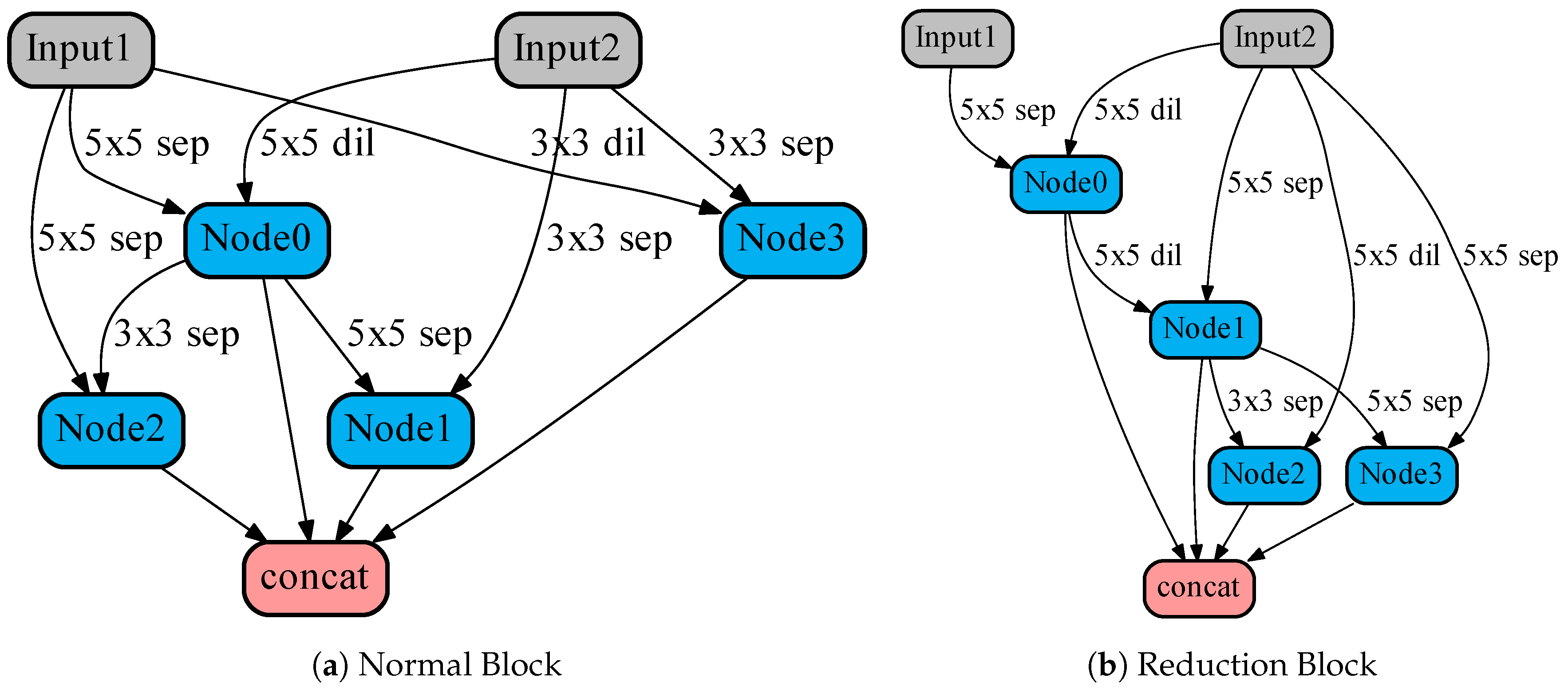
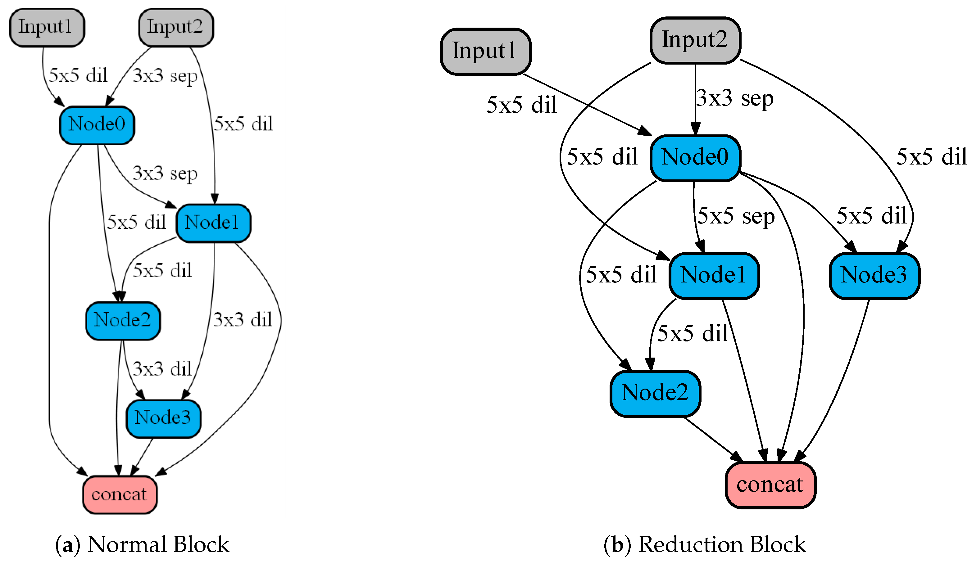
Figure 6 shows the structure of normal block and reduction block searched on MTARSI dataset. Similarly, the scale is more abundant for normal block while the reduction block has a preference for convolutions with large receptive field. Meanwhile, perhaps for the purpose of reducing the computation, we also observe that depthwise separable convolutions are frequently selected in most edges of these two kinds of blocks.
In order to confirm the performance of FGATR-Net on MTARSI dataset, we also compare it with some popular neural networks. All results are listed in Table 1. The confidence interval under the confidence degree of 95% is ± 0.14 . FGATR-Net outperforms other manual models with much fewer parameters. Here, all baseline models load pretrained weights on ImageNet [38] while FGATR-Net is just trained from scratch. As for the comparison of EfficientNet [29], an excellent baseline model obtained by search approach not only in recognition performance but also in lightweight, FGATR-Net also performs well. There are about four percentage points increase in OA, yet the parameters are reduced by almost a half. As a result, we can draw an important conclusion that the proposed automatic design pattern provides a more flexible connection selection for the neural network. In this approach, there is no need to follow more regular topology rules which involve many artificial factors. Therefore, the topology diversity of neural network is increased, which is conducive to explore the optimal architecture.
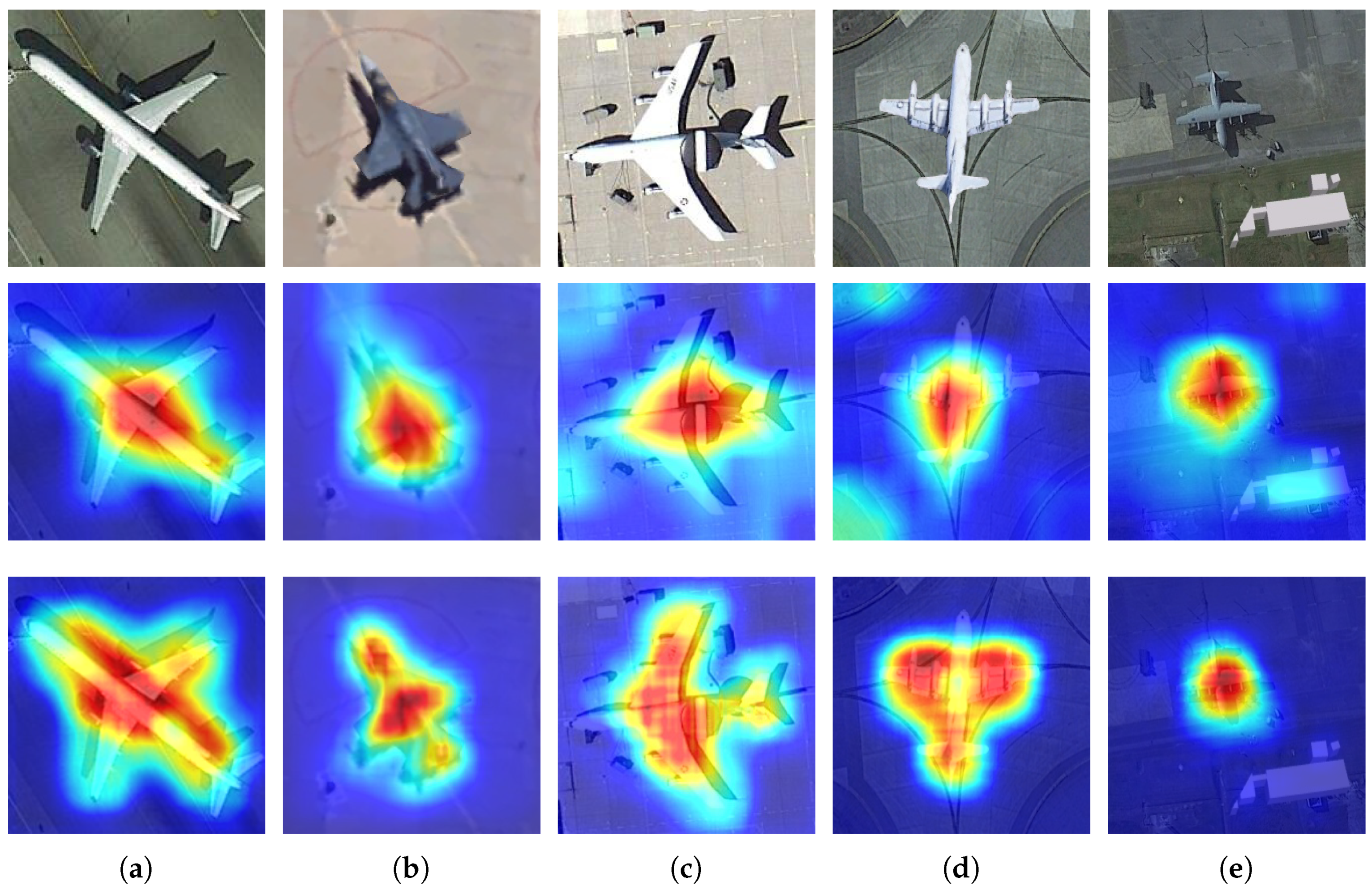
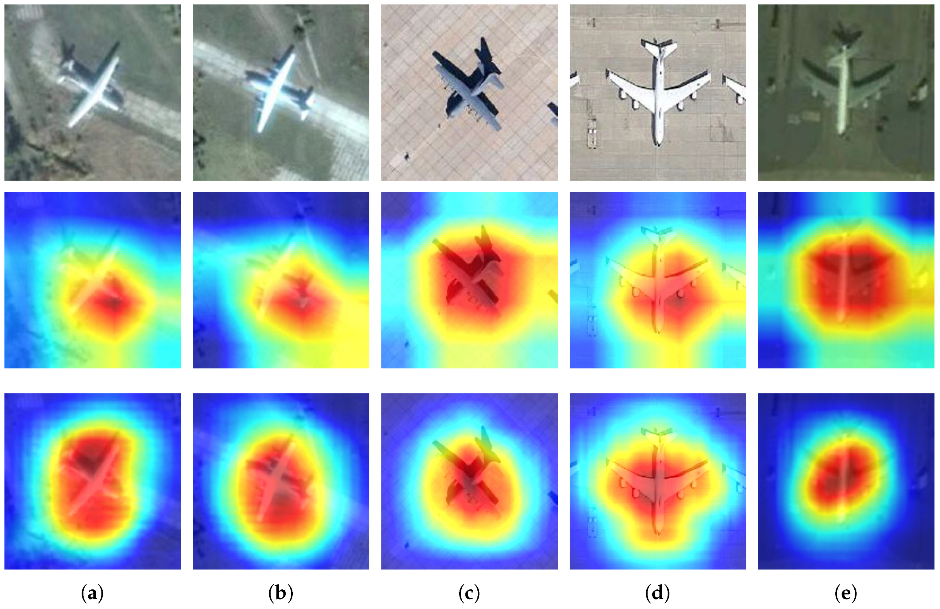
Figure 7 shows some Class Activation Map (CAM) [39] examples on MTARSI dataset. CAM is a visualization method which can reflect the more concerned part of a neural network and then can affect its final decision. The red region indicates a high degree of concern while the model pays a relatively low attention to the blue region. We can observe that compared with EfficientNet, FGATR-Net can manage to capture the key region whether the scale of aircraft in images is large or small. For instance, Figure 7a,c respectively present a large aircraft while a small aircraft is shown in Figure 7e. EfficientNet only focuses on small scale aircrafts. On the contrary, FGATR-Net is able to cover all of them. We infer that this phenomenon is caused by the huge difference between remote sensing images and natural scene images. EfficientNet is more suitable for processing natural scene images, but not for remote sensing images. Moreover, FGATR-Net also has strong robustness to the brightness of remote sensing images, such as Figure 7c,e. Even more importantly, FGATR-Net searched on MTARSI can still better express the outline of aircraft. The boundary information and details are more obvious. This is a powerful support for the feature extraction and feature expression of the proposed FGATR-Net.

4.2. Results on Aircraft17

Architectures for Aircraft17 dataset searched by the proposed method are shown in Figure 8. The search procedure took about two hours on three RTX 2080Ti with batch size 12. From the results of normal block, we can find that there are many types of convolutions. It is helpful to extract multi-scale information for neural network through various convolutions. While for reduction block, 5 × 5 dilated convolution are preferred. This indicates that the network has a strong demand for a relatively large receptive field.
With regard to quantitative experiments, we list the results in Table 2. The confidence interval under the confidence degree of 95% is ± 0.42 . As can be seen in it, FGATR-Net is superior to all baseline models and achieves the highest OA. Similarly, baseline networks all include pretrained model and FGATR-Net is just trained on Aircraft17 dataset from scratch. This suggests that FGATR-Net has a good performance on feature extraction. Moreover, it also performs well in terms of lightweight. The number of parameters FGATR-Net contains is only 1.86 MB, reducing about 25% parameters compared with ShuffleNetV2 [11] which is a very famous lightweight neural network. This strongly indicates that the architecture is relatively more compact. Here, it is remarkable that the architecture design is just an automatic procedure and this procedure does not need much expert knowledge and expert experience. Yet, some promising results can still be obtained from this automatic framework.
In addition to the quantitative results above, the visualization results, i.e., CAMs, on Aircraft17 dataset are also presented in Figure 9. We compare the best performing baseline model, DenseNet, and the proposed FGATR-Net. We find that the salient regions obtained by DenseNet, namely deep red part in CAMs, either has an obvious offset of the aircraft or covers the aircraft area excessively. However, the corresponding CAMs of FGATR-Net almost manges to cover the aircraft area in remote sensing images. It suggests that the proposed FGATR-Net is able to effectively extract the vital information in main region, which verifies the effectiveness of our method.

5. Discussion

The experimental results show that the proposed FGATR-Net is a very competitive model. It is able to extract the key features in remote sensing images and express them well. From the perspective of both OA metric and parameter quantity, it achieves State Of The Art (SOTA) performance on two quite challenging datasets: MTARSI and Aircraft17 respectively. Besides, it is worth noting that our network architecture design is an automatic approach. It does not heavily rely on expert knowledge and artificial experience. Our method provides a new pattern for fine-grained visual classification in remote sensing images.
Table 3 lists the selected pruning strategies at different phases on Aircraft17 and MTARSI respectively. We can observe that greedy strategy and ϵ -greedy strategy are selected successively during search on Aircraft17 dataset. We think that network architecture is relatively shallow at the beginning of the search process. The combination of all candidate functions is limited. Thus, exploitation is favored. However, as the network architecture deepens and search space still contains more elements, the combination becomes complicated. Exploration probably could be a better choice. On the contrary, for MTARSI, ϵ -greedy strategy is selected only. This is most likely caused by relatively large-scale dataset (9385 remote sensing images in this dataset). Information obtained during search is not sufficient enough, making exploration more effective.
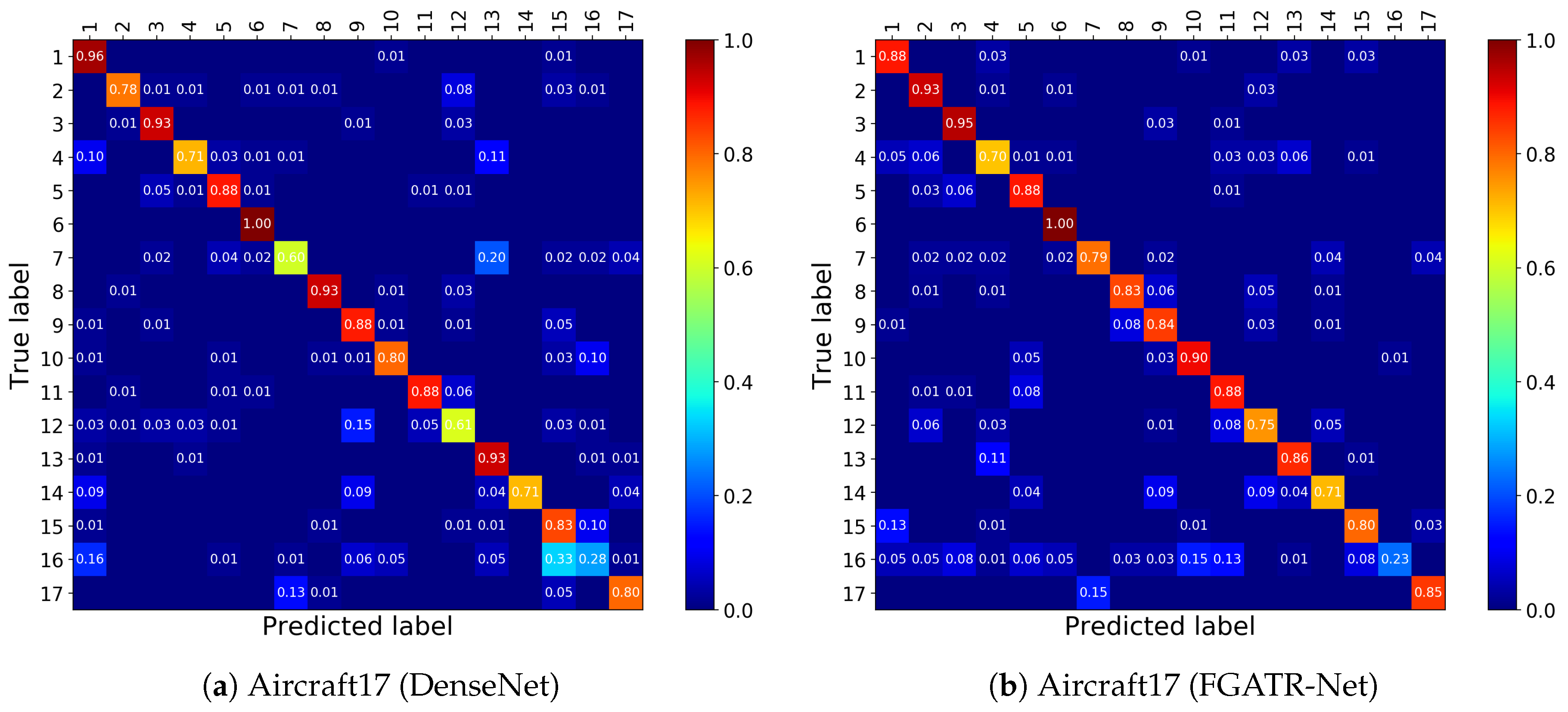
From the confusion matrix results in Figure 10, we observe that most types of aircrafts can be correctly distinguished on Aircraft17 dataset. The recognition metrics of them are satisfied in principle, especially for type 6 whose accuracy even reaches 100%. Nevertheless, the proposed method can still get some further improvements. We notice that the recognition performance of type 16 is a huge drag on OA metric for the best baseline model (i.e., DenseNet) and the proposed FGATR-Net. In DenseNet model, type 16 is most likely to be identified into type 15 while FGATR-Net possibly recognizes this type as type 10 and type 11.
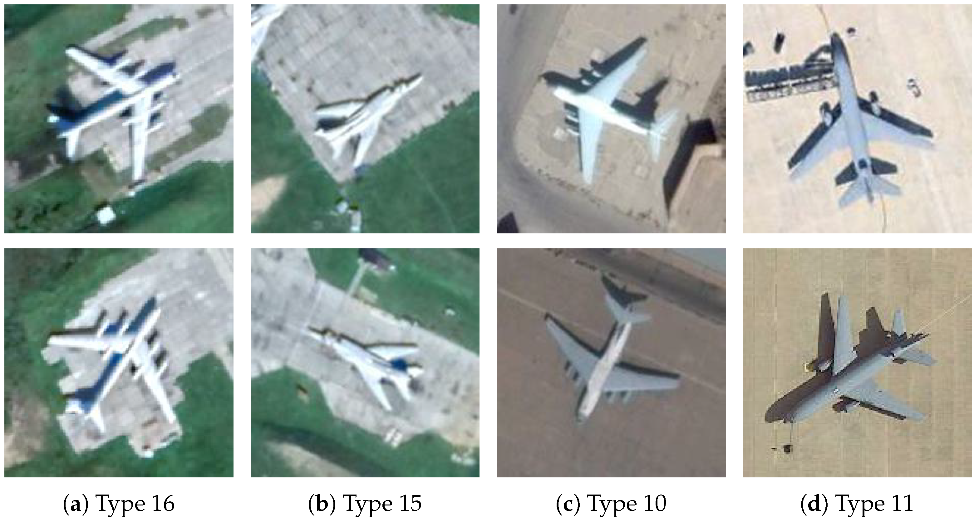
As shown in Figure 11, there is a big difference in aircraft type between type 16 and type 15, yet the background is quite similar for both two types. The background of these images is green and airport runways are light grey. This demonstrates that background is an important influence factor to DenseNet. On the other side, FGATR-Net overcomes this interference. The proportion of being misclassified as type 15 is not very large. However, FGATR-Net has a poor performance for similar aircraft types. There are both 4 engines for type 16 and type 10 while type 16 and type 11 are swept-back wings and their fuselages are relatively long.
In practical application, especially in the military field, a neural network must be robust enough. It can be able to resist external interferences as mentioned above to prevent being deluded. Yet, for the proposed FGATR-Net, there is still room for improvement in this respect. Also, for edge computing devices, it is likely that the hardwares do not perform well as that under experimental conditions. How to keep a good behavior on real-world devices is an important consideration as well for automatic architecture design. Consequently, we will pay more attention to these problems in the future research.

6. Conclusions

In this article, a novel automatic architecture design framework for remote sensing fine-grained aircraft type recognition is firstly explored. In this approach, the search process is divided into several phases. Network architecture deepens at each phase while the number of candidate functions decreases gradually. To achieve it, we adopt different pruning strategies. Then, the network architecture is determined through a potentiality judgment after an architecture heating process. This approach can not only search deeper network, but also reduce the computational complexity, especially for relatively large size of remote sensing images. When the search process is complete, FGATR-Net is obtained and after that we train it on target dataset from scratch. Experimental results on two challenging datasets: MTARSI and Aircraft17 show that FGATR-Net can achieve the highest accuracy, i.e., 93.76% and 81.72% respectively, with just much fewer parameters (2.33 MB and 1.86 MB respectively), compared with popular baseline models, which verifies that FGATR-Net possesses a strong capability of feature extraction and feature representation. Furthermore, it powerfully indicates the feasibility and effectiveness of the proposed automatic architecture design method. As to future work, we will continue to concentrate on automatic and lightweight network design for remote sensing fine-grained aircraft type recognition, and attempt to improve search efficiency while reduce the computational complexity.

Author Contributions

W.L. and J.L. designed and conducted the experiments; W.L. and J.L. reimplemented some popular baseline models. W.L. and J.L. wrote the paper jointly; W.D. and X.S. revised the paper and presented some suggestions; K.F. and Y.W. supervised this research and reviewed this paper. All authors have read and agreed to the published version of the manuscript.

Funding

This work was supported by the National Natural Science Foundation of China under Grants 61725105 and 41701508.

Acknowledgments

The authors would like to appreciate all colleagues in the laboratory, who generously shared their computation resources and gave valuable advice to help us to conduct this research. The authors would also like to sincerely express their gratitude for all anonymous reviewers for their quite helpful suggestions and comments.

Conflicts of Interest

The authors declare no conflict of interest.

References

  1. Chen, J.; Zhang, B.; Wang, C. Backscattering feature analysis and recognition of civilian aircraft in TerraSAR-X images. IEEE Geosci. Remote Sens. Lett. 2014, 12, 796–800. [Google Scholar] [CrossRef]
  2. Zhong, Y.; Ma, A.; soon Ong, Y.; Zhu, Z.; Zhang, L. Computational intelligence in optical remote sensing image processing. Appl. Soft Comput. 2018, 64, 75–93. [Google Scholar] [CrossRef]
  3. Hsieh, J.W.; Chen, J.M.; Chuang, C.H.; Fan, K.C. Aircraft type recognition in satellite images. IEE Proc. Vis. Image Signal Process. 2005, 152, 307–315. [Google Scholar] [CrossRef] [Green Version]
  4. Xu, C.; Duan, H. Artificial bee colony (ABC) optimized edge potential function (EPF) approach to target recognition for low-altitude aircraft. Pattern Recognit. Lett. 2010, 31, 1759–1772. [Google Scholar] [CrossRef]
  5. Liu, G.; Sun, X.; Fu, K.; Wang, H. Aircraft recognition in high-resolution satellite images using coarse-to-fine shape prior. IEEE Geosci. Remote Sens. Lett. 2012, 10, 573–577. [Google Scholar] [CrossRef]
  6. Krizhevsky, A.; Sutskever, I.; Hinton, G.E. Imagenet classification with deep convolutional neural networks. In Proceedings of the Advances in Neural Information Processing Systems, Lake Tahoe, NV, USA, 3–6 December 2012; pp. 1097–1105. [Google Scholar]
  7. Simonyan, K.; Zisserman, A. Very deep convolutional networks for large-scale image recognition. arXiv 2014, arXiv:1409.1556. [Google Scholar]
  8. Szegedy, C.; Liu, W.; Jia, Y.; Sermanet, P.; Reed, S.; Anguelov, D.; Erhan, D.; Vanhoucke, V.; Rabinovich, A. Going deeper with convolutions. In Proceedings of the IEEE Conference on Computer Vision and Pattern Recognition, Boston, MA, USA, 7–12 June 2015; pp. 1–9. [Google Scholar]
  9. He, K.; Zhang, X.; Ren, S.; Sun, J. Deep residual learning for image recognition. In Proceedings of the IEEE Conference on Computer Vision and Pattern Recognition, Las Vegas, NV, USA, 27–30 June 2016; pp. 770–778. [Google Scholar]
  10. Huang, G.; Liu, Z.; Van Der Maaten, L.; Weinberger, K.Q. Densely connected convolutional networks. In Proceedings of the IEEE Conference on Computer Vision and Pattern Recognition, Honolulu, HI, USA, 21–26 June 2017; pp. 4700–4708. [Google Scholar]
  11. Ma, N.; Zhang, X.; Zheng, H.T.; Sun, J. Shufflenet v2: Practical guidelines for efficient cnn architecture design. In Proceedings of the European Conference on Computer Vision (ECCV), Munich, Germany, 8–14 September 2018; pp. 116–131. [Google Scholar]
  12. Diao, W.; Sun, X.; Dou, F.; Yan, M.; Wang, H.; Fu, K. Object recognition in remote sensing images using sparse deep belief networks. Remote Sens. Lett. 2015, 6, 745–754. [Google Scholar] [CrossRef]
  13. Hinton, G.E.; Salakhutdinov, R.R. Reducing the dimensionality of data with neural networks. Science 2006, 313, 504–507. [Google Scholar] [CrossRef] [Green Version]
  14. Fu, K.; Dai, W.; Zhang, Y.; Wang, Z.; Yan, M.; Sun, X. Multicam: Multiple class activation mapping for aircraft recognition in remote sensing images. Remote Sens. 2019, 11, 544. [Google Scholar] [CrossRef] [Green Version]
  15. Zhao, A.; Fu, K.; Wang, S.; Zuo, J.; Zhang, Y.; Hu, Y.; Wang, H. Aircraft recognition based on landmark detection in remote sensing images. IEEE Geosci. Remote Sens. Lett. 2017, 14, 1413–1417. [Google Scholar] [CrossRef]
  16. Zhang, Y.; Sun, H.; Zuo, J.; Wang, H.; Xu, G.; Sun, X. Aircraft type recognition in remote sensing images based on feature learning with conditional generative adversarial networks. Remote Sens. 2018, 10, 1123. [Google Scholar] [CrossRef] [Green Version]
  17. Wang, T.C.; Liu, M.Y.; Zhu, J.Y.; Tao, A.; Kautz, J.; Catanzaro, B. High-resolution image synthesis and semantic manipulation with conditional gans. In Proceedings of the IEEE Conference on Computer Vision and Pattern Recognition, Salt Lake City, UT, USA, 18–23 June 2018; pp. 8798–8807. [Google Scholar]
  18. Zoph, B.; Le, Q.V. Neural architecture search with reinforcement learning. arXiv 2016, arXiv:1611.01578. [Google Scholar]
  19. Zoph, B.; Vasudevan, V.; Shlens, J.; Le, Q.V. Learning transferable architectures for scalable image recognition. In Proceedings of the IEEE Conference on Computer Vision and Pattern Recognition, Salt Lake City, UT, USA, 18–23 June 2018; pp. 8697–8710. [Google Scholar]
  20. Liu, H.; Simonyan, K.; Vinyals, O.; Fernando, C.; Kavukcuoglu, K. Hierarchical representations for efficient architecture search. arXiv 2017, arXiv:1711.00436. [Google Scholar]
  21. Real, E.; Aggarwal, A.; Huang, Y.; Le, Q.V. Regularized evolution for image classifier architecture search. In Proceedings of the AAAI Conference on Artificial Intelligence, Honolulu, HI, USA, 27 January–1 February 2019; Volume 33, pp. 4780–4789. [Google Scholar]
  22. Liu, H.; Simonyan, K.; Yang, Y. Darts: Differentiable architecture search. arXiv 2018, arXiv:1806.09055. [Google Scholar]
  23. Chen, X.; Xie, L.; Wu, J.; Tian, Q. Progressive differentiable architecture search: Bridging the depth gap between search and evaluation. In Proceedings of the IEEE International Conference on Computer Vision, Seoul, Korea, 27 October–2 November 2019; pp. 1294–1303. [Google Scholar]
  24. Hochreiter, S.; Schmidhuber, J. Long short-term memory. Neural Comput. 1997, 9, 1735–1780. [Google Scholar] [CrossRef] [PubMed]
  25. Chen, Y.; Zhu, K.; Zhu, L.; He, X.; Ghamisi, P.; Benediktsson, J.A. Automatic design of convolutional neural network for hyperspectral image classification. IEEE Trans. Geosci. Remote Sens. 2019, 57, 7048–7066. [Google Scholar] [CrossRef]
  26. Zhang, M.; Jing, W.; Lin, J.; Fang, N.; Wei, W.; Woźniak, M.; Damaševičius, R. NAS-HRIS: Automatic design and architecture search of neural network for semantic segmentation in remote sensing images. Sensors 2020, 20, 5292. [Google Scholar] [CrossRef]
  27. Krizhevsky, A.; Hinton, G. Learning Multiple Layers of Features from Tiny Images; Technical Report; University of Toronto: Toronto, ON, Canada, 2009. [Google Scholar]
  28. Wu, Z.Z.; Wan, S.H.; Wang, X.F.; Tan, M.; Zou, L.; Li, X.L.; Chen, Y. A benchmark data set for aircraft type recognition from remote sensing images. Appl. Soft Comput. 2020, 89, 106132. [Google Scholar] [CrossRef]
  29. Tan, M.; Le, Q.V. Efficientnet: Rethinking model scaling for convolutional neural networks. arXiv 2019, arXiv:1905.11946. [Google Scholar]
  30. Rumelhart, D.E.; Hinton, G.E.; Williams, R.J. Learning representations by back-propagating errors. Nature 1986, 323, 533–536. [Google Scholar] [CrossRef]
  31. Anandalingam, G.; Friesz, T.L. Hierarchical optimization: An introduction. Ann. Oper. Res. 1992, 34, 1–11. [Google Scholar] [CrossRef]
  32. Colson, B.; Marcotte, P.; Savard, G. An overview of bilevel optimization. Ann. Oper. Res. 2007, 153, 235–256. [Google Scholar] [CrossRef]
  33. Ioffe, S.; Szegedy, C. Batch normalization: Accelerating deep network training by reducing internal covariate shift. arXiv 2015, arXiv:1502.03167. [Google Scholar]
  34. Srivastava, R.K.; Greff, K.; Schmidhuber, J. Training very deep networks. In Proceedings of the Advances in Neural Information Processing Systems, Montreal, QC, Canada, 7–12 December 2015; pp. 2377–2385. [Google Scholar]
  35. Sutton, R.S.; Barto, A.G. Reinforcement Learning: An Introduction; MIT Press: Cambridge, MA, USA, 2018. [Google Scholar]
  36. Qian, N. On the momentum term in gradient descent learning algorithms. Neural Netw. 1999, 12, 145–151. [Google Scholar] [CrossRef]
  37. Kingma, D.P.; Ba, J. Adam: A method for stochastic optimization. arXiv 2014, arXiv:1412.6980. [Google Scholar]
  38. Deng, J.; Dong, W.; Socher, R.; Li, L.J.; Li, K.; Fei-Fei, L. Imagenet: A large-scale hierarchical image database. In Proceedings of the 2009 IEEE Conference on Computer Vision and Pattern Recognition, Miami, FL, USA, 20–25 June 2009; pp. 248–255. [Google Scholar]
  39. Zhou, B.; Khosla, A.; Lapedriza, A.; Oliva, A.; Torralba, A. Learning deep features for discriminative localization. In Proceedings of the IEEE Conference on Computer Vision and Pattern Recognition, Las Vegas, NV, USA, 27–30 June 2016; pp. 2921–2929. [Google Scholar]
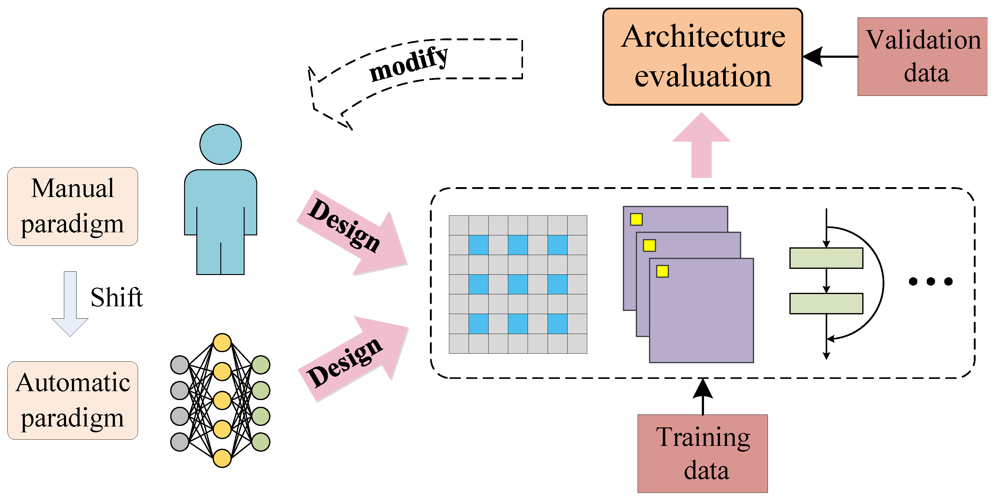
Figure 1. An illustration of manual and automatic architecture design paradigm. The upper part is the manual paradigm where a network architecture is modified through handcraft approach. It needs plentiful experience and knowledge. While the bottom part is the automatic paradigm where the network can be adjusted by the machine itself. This approach can shift the network design paradigm and save valuable human resources.
Remotesensing 12 04187 g001
Figure 2. The difference between previous search framework for natural scene images and our framework for fine-grained aircraft type recognition in remote sensing images.
Remotesensing 12 04187 g002
Figure 3. The overview of the proposed method. For convenience, we just show part of candidate functions in the predefined search space and pruning phases. Scissors symbols in the figure above denote the pruning process. Stem denotes a simple 3 × 3 convolution module which shifts the number of image channels and reduces the size of image. Architectures with different colors represent different depths. Best viewed in color.
Remotesensing 12 04187 g003
Figure 4. Some samples of MTARSI dataset.
Remotesensing 12 04187 g004
Figure 5. Some samples of Aircraft17 dataset.
Remotesensing 12 04187 g005
Figure 6. Architectures searched on MTARSI dataset. Legend—Node: input nodes; Node: middle nodes; Node: output nodes. Best viewed in color.
Remotesensing 12 04187 g006
Figure 7. Several CAMs on MTARSI dataset. From subfigure (a) to subfigure (e), raw remote sensing images are arranged in the first row while the corresponding CAMs of EfficientNet and FGATR-Net are placed in the second row and third row respectively.
Remotesensing 12 04187 g007
Figure 8. Architectures searched on Aircraft17 dataset. Legend—Node: input nodes; Node: middle nodes; Node: output nodes. Best viewed in color.
Remotesensing 12 04187 g008
Figure 9. Several CAMs on Aircraft17 dataset. From subfigure (a) to subfigure (e), raw remote sensing images are arranged in the first row while the corresponding CAMs of DenseNet and FGATR-Net are placed in the second row and third row respectively.
Remotesensing 12 04187 g009
Figure 10. Confusion matrices of DenseNet and FGATR-Net on Aircraft17 dataset.
Remotesensing 12 04187 g010
Figure 11. Some examples which are easily to be confused in Aircraft17 dataset.
Remotesensing 12 04187 g011
Table 1. Recognition results and parameter quantity on MTARSI.
NetworkMethodOA (%)Param (MB)
AlexNet [28]Manual85.6157.09
VGGNet [28]Manual87.56134.34
GoogLeNet [28]Manual86.535.62
ResNet [28]Manual89.6123.55
DenseNet [28]Manual89.156.97
EfficientNet [28]Automatic89.794.03
FGATR-NetAutomatic93.762.33
Table 2. Recognition results and parameter quantity on Aircraft17. NC means not-convergent.
NetworkMethodOA (%)Param (MB)
AlexNet [6]Manual70.3057.07
VGGNet [7]ManualNC134.33
GoogLeNet [8]Manual71.135.62
ResNet [9]Manual77.8823.54
DenseNet [10]Manual80.486.97
ShuffleNetV2 [11]Manual73.942.50
FGATR-NetAutomatic81.721.86
Table 3. Selected pruning strategies at different search phases on two datasets.
Search PhaseAircraft17MTARSI
Phase IPhase IIPhase IPhase II
greedy strategy
ϵ -greedy strategy
Publisher’s Note: MDPI stays neutral with regard to jurisdictional claims in published maps and institutional affiliations.