Weed Identification in Maize, Sunflower, and Potatoes with the Aid of Convolutional Neural Networks

Abstract

The increasing public concern about food security and the stricter rules applied worldwide concerning herbicide use in the agri-food chain, reduce consumer acceptance of chemical plant protection. Site-Specific Weed Management can be achieved by applying a treatment only on the weed patches. Crop plants and weeds identification is a necessary component for various aspects of precision farming in order to perform on the spot herbicide spraying or robotic weeding and precision mechanical weed control. During the last years, a lot of different methods have been proposed, yet more improvements need to be made on this problem, concerning speed, robustness, and accuracy of the algorithms and the recognition systems. Digital cameras and Artificial Neural Networks (ANNs) have been rapidly developed in the past few years, providing new methods and tools also in agriculture and weed management. In the current work, images gathered by an RGB camera of Zea mays, Helianthus annuus, Solanum tuberosum, Alopecurus myosuroides, Amaranthus retroflexus, Avena fatua, Chenopodium album, Lamium purpureum, Matricaria chamomila, Setaria spp., Solanum nigrum and Stellaria media were provided to train Convolutional Neural Networks (CNNs). Three different CNNs, namely VGG16, ResNet–50, and Xception, were adapted and trained on a pool of 93,000 images. The training images consisted of images with plant material with only one species per image. A Top-1 accuracy between 77% and 98% was obtained in plant detection and weed species discrimination, on the testing of the images.

1. Introduction

Public concern about food security has increased in the last decades. Simultaneously, stricter rules have been applied worldwide regarding pesticide usage in the agri-food chain. The above reasons have reduced the consumer acceptance of chemical plant protection. Site-Specific Weed Management can be achieved by applying a treatment only on the weed patches. The current application methodology is to spread the herbicide on the whole field [1], which involves a portion of the herbicide to be applied to non-target plants as weeds have a variable and heterogeneous distribution over the field [2,3]. Thus, the current state of application technology usually has a low degree of the effectiveness of the treatment while it simultaneously leads to an unnecessary negative input into the environment [4]. Yet, reducing the spray rate is not advisable for agronomical reasons, since it can promote the emergence of resistant weed species, while it can also lead to a decrease in yield [5].

As Dyrmann et al. [6] predicted, using herbicides will be a challenging approach under the increasing political and social pressure. Therefore, the reduction of herbicides, insecticides, and fungicides is a major motivating force behind current agricultural expert systems [7,8] to comply with EU Directive 2009/128/EC [9]. On that front, precision farming or smart farming has improved the potentials of automation in agricultural applications [10,11,12]. Tyagi [11] has especially made great progress in the automation of agriculture applications. Due to this effort, robots applying pesticides on a plant individual level might soon be implemented as the standard application technology [13]. Crop and weed recognition foremost, and weed diversification secondary, are key elements for automating the weed management technologies and achieve successful weed control [14]. They are a prerequisite for further expansion towards a more sustainable agriculture. Targeted treatments, chemical or mechanical, can achieve better results if the treatment is targeted only on the weeds, and if we can diversify our treatment (e.g., different herbicide) based on the specific weed class [15]. A detailed plant mapping of the field can give a valuable insight into the specific weed population and the coverage of each species, which can lead to a more sophisticated weed management treatment and more educated weed management strategies.

Convolution neural networks (CNNs)—first implemented by LeCun et al. [16]—can be used as a tool providing highly-accuracy concerning image classification, object detection, and can even be a valuable candidate for fine-grained classification [17]. Although the use of CNNs is relatively new, recent publications have reached high classification accuracies of 99.50% for classifying segments as crop, soil, grass, and broadleaf weeds [15], 96.10% on a blob-wise crop/weed classification [18], 94.38% between twelve different plant species [19], and 95.70% of eight Australian weed species [20]. CNNs can provide insights into image related datasets that we have not yet understood, achieving identification accuracies that sometimes surpass the human-level performance [21]. When given sufficient data, the deep learning approach generates and extrapolates new features without having to be explicitly told which features should be used and how they should be extracted [22,23,24]. One of the most important characteristics of using CNNs in image processing is the obsolescence of feature engineering [25] as the CNN can obtain essential features by itself [26]. It can build and utilize more abstract concepts [27]. Therefore, with the utilization of deep learning procedures and CNNs in image processing, there is a reduced need to manually produce the best features [25,28]. Furthermore, these self-learned features make the deep learning approach less effective for natural variations such as changes in illumination, shadows, skewed leaves, and occluded plants, provided that the used methods have been trained partially or fully in a high variability of these different input variations [6]. Hence, state-of-the-art CNNs with a classification accuracy of over 95% on specific tasks are now quite close to human performance [29]. In agriculture and specifically in weed identification, the ability of CNNs to learn and obtain features in combination with their lower effect on natural variations makes these methods quite promising and able to achieve better classification results from other solutions.

According to Rawat and Wang [21], the deep learning renaissance was fueled by advanced hardware and improved algorithms. The usage of deep learning has swiftly emerged as a promising method in weed and plant classification, although it remains a relatively new topic as most publications were published after 2016 [25]. This is mainly the case because a lot of resources are required to create a large multi-class dataset for plant and weed classification [25,30,31], especially if the dataset is acquired under field conditions. Nevertheless, CNNs—which have been widely used in image recognition tasks—have swiftly emerged as a promising method in weed and plant classification in recent years.

In 2016, using a CNN, Dyrmann et al. [6] proposed a state-of-the-art approach in plant species classification. They built their own CNN and trained it using mini batches with 200 images. Their network was able to classify 22 weed and crop species from BBCH 12-16 [32] with an accuracy of 86.2%. Their dataset underlines the importance of adequate images for each species because if the amount of data is insufficient the recognition rate will significantly decline. Elnemr [19] proposed a new simple self-built CNN architecture to classify twelve classes (three crops and nine weeds) during their early growth stages. The results indicate that the more classes that the training dataset comprises, the more difficult it is to reach a good classification result. Nevertheless, the twelve-class CNN achieved an average test accuracy of 94.38%. Besides training and building a CNN from scratch, Ge et al. [33] proposed that when the dataset is limited it is better to take a pretrained network, trained on a large dataset such as ImageNet, and apply transfer learning [34] to reach a better performance and reduce overfitting. dos Santos Ferreira et al. [15] used a replication of AlexNet, pretrained on the ImageNet dataset for their neural network. Four classes were distinguished—soil, Glycine max, grass, and broadleaf weeds—from drone data, and the network reached an average accuracy of 99.5%. Munz and Reiser [35] used some pre-trained networks not only to separate between pea and oat but to also estimate their coverage. Olsen et al. [20] trained multiple CNNs: Inception-v3 [36] based on GoogLeNet [37] and ResNet–50 [38], both pretrained with the ImageNet dataset. In addition to the comparison of different CNNs, they introduced the first large, multi-class weed species image dataset (Deepweeds), comprising eight invasive weed species and collected entirely under field conditions. The networks were trained for 100 epochs and achieved average classification results of 95.1% (Inception-v3) and 95.7% (ResNet–50), respectively.

Each author either constructed their own network from scratch or used existing architectures that were modified for the respective dataset. In all cases, the authors have demonstrated the potential use of Neural Networks also in the agricultural discipline. Nevertheless, choosing a suitable network requires careful planning as it must fit the task at hand [39]. Furthermore, the robustness of the trained network, along with the robustness of training similar networks has not been examined. In the context of weed and crop classification, supervised training with a prelabeled dataset is widely used to cope with the high variability in the morphology of the plants based on the development stages and environmental influence, which can lead to poor classification accuracy [39]. Yet, the difficulty of acquiring multiple labeled instances of each plant in different development stages still poses an important academic and practical challenge [20]. The acquired datasets typically have a small number of labels, and a huge variation between the classes, which enforce the usage of an unbalanced dataset. In the current paper, the capabilities of three different networks were examined, namely VGG16 [40], ResNet–50 [38] and Xception [41] in their capabilities of identifying twelve different plant species. Our aim was to demonstrate how fast those networks can be trained, and how reliable this training can be, over multiple trainings. Through the proposed methodology a significant amount of labeled images have been acquired that enabled the utilization of a balanced subset of the dataset for training and validation purposes. Ten different repetitions of each network were performed to examine if the CNN training can always conclude to similar results, in a standardized and systematic way. Therefore, we tried to investigate if this balanced dataset can achieve a better result in weed identification and plant classification than the previously demonstrated, for an agronomically applicable amount of classes.

2. Materials and Methods

2.1. Experimental Field

Images were gathered on a predefined experimental field at the Heidfeldhof research station of the University of Hohenheim, in southwest Germany (48°42${}^{\prime }$59.0${}^{″}$N and 9°11${}^{\prime }$35.4${}^{″}$E) in 2019. Twelve plots of 12.5 × 1 m were used, each seeded with the seeds of the respective plant species. Three crop species were used, namely maize (Zea mays L.), potato (Solanum tuberosum L.), and sunflower (Helianthus annuus L.) along with nine weed species, namely Alopecurus myosuroides Huds, Amaranthus retroflexus L., Avena fatua L., Chenopodium album L., Lamium purpureum L., Matricaria chamomila L., Setaria spp., Solanum nigrum L., and Stellaria media Vill. (

Table 1. Plant species used in the training of the CNNs, the relevant EPPO code, along with the number of labels per plant species in total and for the training, validation and training subset.

Plant Species	EPPO CODE	Total Images	Train Images	Validation Images	Testing Images
Alopecurus myosuroides Huds.	ALOMY	7423	5196	1113	1114
Amaranthus retroflexus L.	AMARE	5274	3691	791	792
Avena fatua L.	AVEFA	12,409	8686	1861	1862
Chenopodium album L.	CHEAL	2690	1882	403	405
Helianthus annuus L.	HELAN	16,426	11,498	2463	2465
Lamium purpureum L.	LAMPU	7603	5322	1140	1141
Matricaria chamomila L.	MATCH	15,159	10,611	2273	2275
Setaria spp. L.	SETSS	2378	1664	355	359
Solanum nigrum L.	SOLNI	2979	2085	446	448
Solanum tuberosum L.	SOLTU	2742	1919	411	412
Stellaria media Vill.	STEME	6941	4858	1041	1042
Zea mays L.	ZEAMX	11,106	7774	1665	1667
	SUM	93,130	65,186	13,962	13,982

). In the current work, plant species will refer to both crop and weed data; otherwise, it will be explicitly stated as crop or weed plants. Images were gathered every second day from the date of emergence for 45 days until the plants had progressed to the 8th leave stage or the beginning of tillering. Prior to the seeding, the soil was cultivated in spring with a Rabe cultivator and a working width of 3 meters, and the field was sterilized with a steam treatment to reduce the emergence of unwanted weeds and volunteer previous crop plants. Furthermore, the experimental plots were cleaned by hand from weeds foreign to the intended species twice a week.

2.2. Image Acquisition

The pictures were captured with a Sony Alpha 7R Mark4 (ILCE7-RM4, Sony Corporation, Tokyo, Japan ), a 61 megapixel RGB DSLR camera at noon. The camera has a 35.7 × 23.8 mm, back illuminated full frame CMOS sensor and JPEG images were taken at a resolution of 9504 × 6336 pixels. A shutter speed of 1/2500 s was used, while the ISO calibrated automatically to achieve a good image quality under the changing lighting conditions during the measurements, and the glare opening adjusted each recording day and set between 7 and 11. The Zeiss Batis 25 mm—a fixed focal length lens—was used to achieve a better optical quality compared to a zoom lens. The Sony camera was mounted on the “Sensicle” [42], a multisensor platform for precision farming experiments at a height of 1.2 m. The driving speed was 4 km/h and each second a picture was captured.

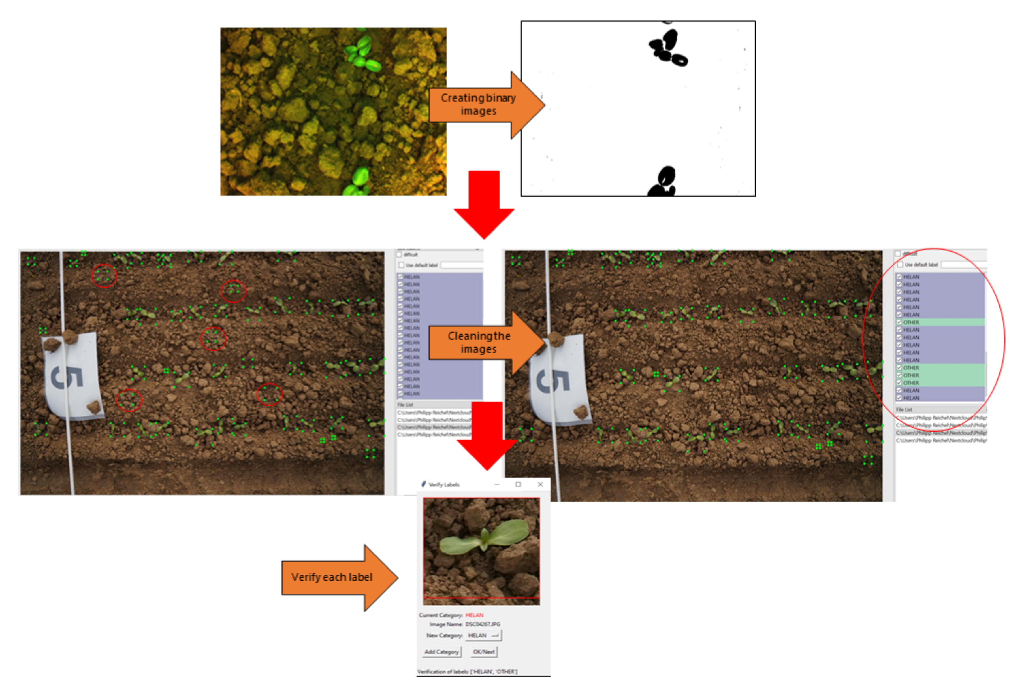
2.3. Image Preprocessing

From each plot, images were saved with information relevant to the plot and acquisition date. For each image, a binary image was created (Figure 1), using the Excess Green–Red Index as a thresholding mechanism to separate plant material from the soil [43,44]. Each connected pixel formation from this thresholding procedure consisted of a potential region of interest that should be fed in the CNNs and was separated and prelabeled, creating the relevant bounding box, based on the following rules:

• Pixel formations less than 400 pixels were discarded.
• Bounding boxes were expanded if needed symmetrically to the minimum size of 64 × 64 pixels. The minimum bounding box was 64 × 64 pixels.
• Regions bigger than 64 pixels were expanded only by 5 pixels in all directions. Therefore, there was no limitation to the maximum box.
• If bounding boxes overlapped, a new bounding box was created, merging all the overlapping boxes.
• Both the original and the merged bounding boxes were kept for labeling.

The above procedure ensures that all potential inputs provided for classification from our preprocessing method are available for labeling, while simultaneously reducing as much as possible soil clusters and other noise inferences. Labels with the respective European and Mediterranean Plant Protection Organization (EPPO) code of each plant were put automatically on each bounding box, based on the image information. These labels were examined by a human expert who discarded possible wrong classifications or unwanted weeds (Figure 1).

Figure 1. Schematic presentation of the labeling workflow using the example of Helianthus annuus.

Figure 1. Schematic presentation of the labeling workflow using the example of Helianthus annuus.

The final dataset was cross examined a second time by a human expert for possible fallacies. The final dataset comprised 93,130 verified single plants (Table 1). Some example images that were used for the training of the networks can be seen in Figure 2.

2.4. Neural Networks

Artificial Neural Networks and specifically Convolutional Neural Networks (CNNs) are a powerful technique that can achieve a successful plant and weed identification. The basic structure of a neural network comprises an input layer, multiple hidden layers, and an output layer. For the current study CNNs that have demonstrated some good or robust results over different disciplines have been selected. Specifically, we used VGG16, ResNet–50, and Xception, as our basic networks, modifying the top layer architecture of each network.

2.4.1. VGG16

Simonyan and Zisserman [40] proposed VGG16, as a further development of AlexNet. VGG16 was one of the best performing networks at the 2014 ImageNet Large Scale Visual Recognition Challenge (ILSVRC) competition, providing a 71.3% top-1 accuracy and a 90.1% top-5 accuracy. ImageNet is a labeled dataset including over 14 million images classified to 1000 different classes. VGG16 has been used for its robustness since it can provide a high performance and respective accuracies, even when the image datasets are small [45]. The input of VGG16 is a three channel RGB image of the fixed size of 224 × 224 pixels. The VGG16 architecture contains a total of 16 layers, comprising 13 convolutional (3 × 3) and three fully-connected layers (

Table 2. General information about the three neural networks used.

	VGG16	ResNet–50	Xception
Mean time per epoch (s)	164	164	274
Minimum epochs used	469	511	538
Maximum epochs used	864	979	945
Minimum top—1 test accuracy [%]	81	97.2	97.5
Maximum top—1 test accuracy [%]	82.7	97.7	97.8
Minimum final validation loss	0.524	0.077	0.085
Maximum final validation loss	0.560	0.089	0.097
Network Depth (Layers)	16	50	71
Total Network Parameters	27,829,068	24,905,612	22,179,380
Trained network parameters	13,114,380	1,371,020	1,372,428
Input Image Size (pixels)	224 × 224	224 × 224	299 × 299
Batch Size	32
Train Images per epoch	15,600
Validation Images per epoch	4200

). Rectified linear units (ReLUs)—first presented by Krizhevsky et al. [46]—act as the activation function for each convolutional layer and for the first two fully-connected layers. VGG16 is one of the best performing networks from the last years, but simultaneously it is simpler, less computer intensive than other networks.

2.4.2. ResNet–50

ResNet–50 (Residual Network 50) was first presented by He et al. [38]. Their architecture continued with the trend of an increased layer depth. ResNet–50 has a similar architecture as VGG16, centered around a 3 × 3 convolutional layer with a ReLU activation function, but before and after each 3 × 3 convolutional layer 1 × 1 convolutional layers are established. Furthermore, only one pooling layer is used, batch normalization is implemented, and the final total network structure comprised three times more layers than VGG16. It is comparable to the VGG16 network, apart from the fact that Resnet50 has an additional identity mapping capability [45]. ResNet–50 can be trained much faster than the VGG16, since it reduces the vanishing gradient problem by creating an alternative shortcut for the gradient to pass trough. Practically this translates as, even if the network is much deeper than VGG16 it can bypass a CNN layer if it is not necessary. The proposed final network comprised of 50 layers (Table 2) and reached first place at the ILSVRC 2015, outperforming the previous benchmark set by VGG16. The input of ResNet–50 is also a three channel RGB image of the fixed size of 224 × 224 pixels. The residual management that ResNet–50 provides makes this algorithm one of the best for training into new datasets.

2.4.3. Xception

Xception [41] stands for Extreme version of Inception and, of course, is an adaptation from Inception, revolutionizing how CNNs are designed. ResNet–50 tried to solve the image classification problem by increasing the depth of the network. The Inception architectures follow a different approach, by increasing the width of the network. A generic Inception module tries to calculate multiple different layers over the same input map in parallel, cleverly merging their results into the output. Three different convolutional layers and one max pool layer are activated in parallel, generating a wider CNN compared with the previous networks. Each output is then combined in a single concatenate layer. Therefore, for each layer, Inception does a 5 × 5, 3 × 3, and 1 × 1 convolutional transformation, and an additional max pool. The concatenate layer of the model then decides whether and how the information of each layer can be used. In Xception, the inception modules have been replaced with depth-wise separable convolutions. It calculates the spatial correlations on each output channel independently of the others, but in the end, it performs a 1 × 1 depthwise convolution to capture the cross-channel correlation. In the end, Xception has also a deep architecture, even deeper than ResNet–50 with 71 layers depth (Table 2). The input of Xception also differs from the two previews networks as it is a three layer RGB image of the fixed size of 299 × 299 pixels, compared to the 224 × 224 that was used before. The width approach that Xception is using, increases its degrees of freedom and therefore utilizes the best identification scenarios for the task at hand.

2.4.4. Dataset Normalization

All 93,130 images were separated into 3 distinct datasets for training, validation, and testing of the networks. To achieve a uniform comparison between network repetitions and network architectures the separation was done apriori, before the image enhancement or augmentation. For each separate class of labels, 70% of the images were used for the training of the networks, 15% of the dataset was used for the validation performed in each training, while the remaining 15% consisted of our testing subset, which was used for the final measurements and demonstration of the achieved results.

In order to perform the training and validation of the networks on a normalized dataset, subsampling was performed. A balanced dataset would avoid population bias since in the dataset there are some majority classes with a high amount of labeled images and some minority classes with fewer images. The large number of images in our dataset enabled us to perform this subsampling since even the minority classes had more than 1600 training images per class. Specifically, every five epochs 1300 images per class on the training subset, and 400 images per class on the validation subset were randomly chosen from their respective subsets. This resulted in 15,600 images to be used in each epoch for training and another 4200 for validation. The testing was performed on the complete unbalanced testing subset since this is a representative fraction of the labels actually identified inside the field.

2.4.5. Network Training

The network experimentation was performed with Keras 2.4.3 in python 3.6.8 using the Tensorflow (2.3.0) backend. Transfer learning was used [34]. All the aforementioned networks were used with the pretrained weights from the ImageNet dataset. The layers of those networks were not trained during our experimentation. For each of the used networks, the pretrained variant was used without the top classification layers for the ImageNet classification. Instead, two additional fully connected dense layers of 512 neurons each were included (Figure 3). On both of those layers, a ReLU activation function was implemented, while during the training a 50% neuron dropout was used. The networks were trained on a supercomputer cluster using the NVIDIA^® Tesla Volta V100 PCIe Tensor Core GPU with 12 GB GPU memory (Nvidia Corporation, Santa Clara, California, United States). Instead of the stochastic gradient descent (SGD) algorithm, Adam, an adaptive learning rate algorithm with a learning rate of 1 ×${10}^{-3}$ and a decay of $\frac{0.01}{200}$, was implemented for Xception and ResNet–50. For VGG16, a smaller learning rate was chosen of 1 ×${10}^{-4}$, but with the same decay. Each network was trained ten times, each independent of the previous ones. For the training and validation subsets, data augmentation was also performed to avoid over-fitting and overcome the highly variable nature of the target classification. This would account for variation in parameters like rotation, scale, illumination, perspective, and color. Specifically, rotation of up to 120 degrees, a brightness shift of $\pm 20\%$, a channel shift of $\pm 30\%$, a zoom of $\pm 20\%$ were randomly performed, along with a possible horizontal and vertical flip. A batch size of 32 images was selected. Each network was trained until the validation accuracy did not improve anymore for 150 consecutive epochs. This ensured that the networks have converged to a maximum, while even in the majority classes the probability that each training image has been used at least once on these 150 epochs overpassed 99%. The maximum and minimum number of epochs among the ten repetitions that each network used for its training can be seen in Table 2. Table 2 also shows information about the training such as the mean time used for the training of each epoch, the training parameters of each architecture, etc.

2.5. Evaluation Metrics

In order to evaluate the performance of the respective network classification result, precision, recall, and f1-score were used as proposed by Sokolova and Lapalme [47]. Precision refers to the class conformity of the data labels with the positive labels assigned by the classifier and it is calculated by:

$$Precision={\displaystyle \frac{tp}{tp+fp}}$$

(1)

where $tp$ represents the true positive values, which means the plants belonging to a class that were identified as such, and $fp$ are the false positive values, the plants that do not belong to a class but were identified as such. Recall evaluates the sensitivity of the respective network and was calculated by:

$$Recall={\displaystyle \frac{tp}{tp+fn}}$$

(2)

where $tp$ is similar to Equation (1), and $fn$ represents the false negative values, which means the plants that belong to the class but were not identified as such. f1-score illustrates the ratio between precision and recall via a harmonic mean and was calculated by:

$$f1-score=2\times {\displaystyle \frac{Precision\times Recall}{Precision+Recall}}$$

(3)

where Precision is defined in Equation (1) and Recall is defined in Equation (2).

3. Results

In the current paper, three different networks have been tested to evaluate their performance in a balanced dataset of twelve different plant species. All three networks had their original layers pretrained on the ImageNet dataset, while some additional fully connected layers were included as top layers of the pretrained network. Only these layers were trained to classify and identify our twelve plant classes. Ten different repetitions of each network type were trained until the validation accuracy did not decrease after 150 epochs.

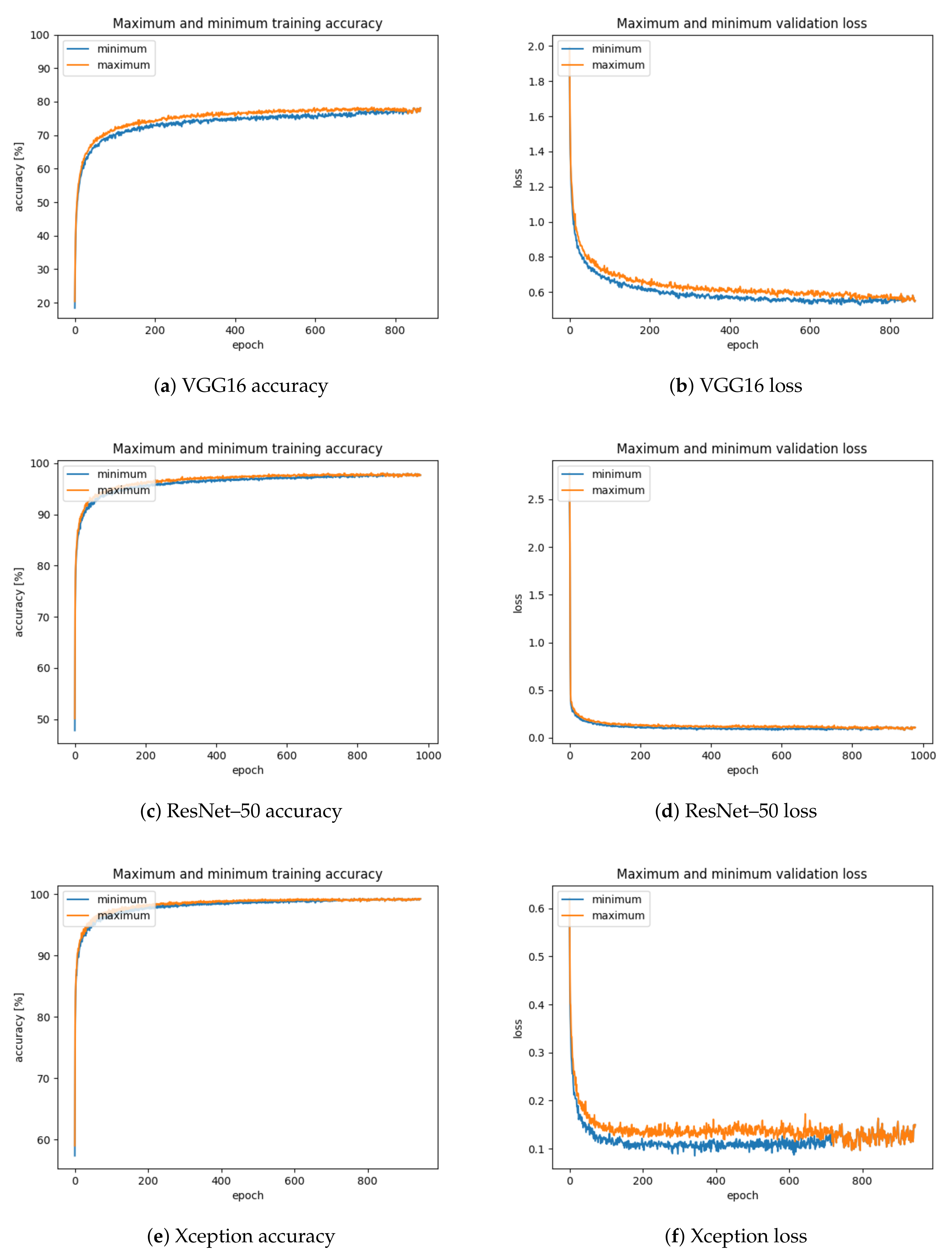
3.1. Model Accuracy/Model Loss

The mean training and valid loss along with the training and validation accuracy per network type can be seen in Figure 4. The training accuracy rapidly increases in the first 100 epochs and then slowly approaches towards an optimum, depending on the network at around 300 to 700 epochs for VGG 16 (Figure 4a), 350 to 850 epochs for ResNet–50 (Figure 4c), and 400 to 800 for Xception (Figure 4e). The model accuracy did not differentiate a lot between the ten repetitions of each network. The biggest differentiation was between the maximum and the minimum accuracy of the VGG 16 Neural Network training. All networks achieved a similar result of around 81% for VGG16 and more than 97% for ResNet–50 and Xception, both in the training and validation accuracy, which was also similar to the testing accuracy performed after the finalization of the training (Figure 4, Table 6). Specifically, the top-1 accuracy for the VGG 16 network ranged from 81 to 82.7%, for ResNet–50 between 97.2 to 97.7%, while the highest accuracy was achieved with Xception at 97.5 to 97.8%.

A loss function is used to improve and evolve the accuracy of a neural network model. Loss functions try to map the parameters of the network onto a single scalar value that indicates how well those parameters achieve in performing the task the network is intended to do. The loss value implies how poorly or well the model behaves after each iteration of optimization. In our case, the model loss is visualized via the sum of errors made for each example in the training or validation set, respectively. The training and validation loss reacted similarly in all networks with the validation loss presenting higher fluctuations and differences than the training loss. The validation loss decreases steadily until it reaches the lowest value depending on the neural network, in similar epochs like the maximum accuracy was achieved. For VGG 16 that was at around 300 to 700 epochs (Figure 4b), 350 to 850 epochs for ResNet–50 (Figure 4d), and 400 to 800 for Xception (Figure 4f). The highest fluctuations between the minimum and the maximum loss difference were monitored for the Xception neural network training while the lowest fluctuations were monitored at the ResNet–50 training.

3.2. Classification Performance

In our dataset, twelve different classes have been used to separate the plants into the equivalent plant species. The distribution of how well the three networks identified each plant species can be seen in

Table 3. Confusion matrix of the mean crop and weed identification for the VGG16 Convolutional Neural Network. The prediction reached between 81.0 and 82.7 % top-1 accuracy on the test dataset. The values are the percentage of identified labels for each plant species (Each row sums to 100%). (a) Mean values for the ten training runs. Cell values above 2% are highlighted. (b) The standard deviation for the ten training runs. Standard deviation values above 0.5% are highlighted.

(a) Mean Values of VGG16
	ALOMY	AMARE	AVEFA	CHEAL	HELAN	LAMPU	MATCH	SETSS	SOLNI	SOLTU	STEME	ZEAMX
ALOMY	86.94	0.16	5.09	0.51	0.00	0.19	0.36	4.95	0.41	0.87	0.06	0.46
AMARE	0.74	92.12	0.06	0.53	0.00	0.76	1.26	3.08	0.47	0.62	0.16	0.19
AVEFA	14.46	0.34	66.57	1.24	0.17	0.41	4.26	2.99	1.83	1.08	0.19	6.45
CHEAL	0.00	4.05	1.51	55.01	0.47	6.74	1.80	2.79	21.60	3.65	1.78	0.59
HELAN	0.29	0.03	0.90	1.35	85.69	0.54	0.55	0.23	0.93	4.04	0.17	5.28
LAMPU	0.17	1.17	0.43	4.96	0.17	75.83	1.82	1.01	7.98	4.80	1.59	0.08
MATCH	1.28	0.89	0.84	0.15	0.00	1.01	93.36	0.88	0.05	0.44	0.70	0.40
SETSS	5.52	7.05	3.59	3.79	0.00	0.89	0.78	74.57	0.50	1.95	1.11	0.25
SOLNI	0.36	2.88	1.90	15.63	0.22	8.08	1.25	0.80	64.26	2.63	1.47	0.51
SOLTU	0.44	0.73	1.21	1.97	1.26	4.64	3.25	0.19	2.14	82.33	0.85	1.00
STEME	0.02	4.99	0.04	3.11	0.00	4.54	2.86	1.90	2.22	1.48	78.69	0.15
ZEAMX	0.56	0.11	6.66	0.97	3.88	0.22	1.33	0.47	1.13	1.93	0.52	82.21
(b) Standard Deviation of VGG16
	ALOMY	AMARE	AVEFA	CHEAL	HELAN	LAMPU	MATCH	SETSS	SOLNI	SOLTU	STEME	ZEAMX
ALOMY	1.23	0.09	0.91	0.10	0.00	0.09	0.17	0.78	0.13	0.19	0.06	0.15
AMARE	0.17	1.50	0.06	0.17	0.00	0.28	0.28	0.91	0.22	0.16	0.11	0.06
AVEFA	1.46	0.17	2.11	0.20	0.06	0.12	0.61	0.43	0.21	0.18	0.07	0.88
CHEAL	0.00	0.71	0.49	3.00	0.26	1.20	0.44	0.48	2.55	0.56	0.62	0.12
HELAN	0.02	0.02	0.11	0.17	0.69	0.11	0.07	0.04	0.14	0.45	0.07	0.51
LAMPU	0.06	0.30	0.13	0.69	0.05	1.46	0.34	0.17	1.28	0.37	0.48	0.03
MATCH	0.28	0.16	0.18	0.05	0.01	0.16	0.52	0.21	0.05	0.11	0.13	0.17
SETSS	1.50	1.47	0.70	0.97	0.00	0.45	0.41	2.24	0.24	0.45	0.51	0.15
SOLNI	0.15	0.59	0.36	2.19	0.00	1.70	0.20	0.36	2.94	0.70	0.29	0.10
SOLTU	0.18	0.24	0.24	0.17	0.26	1.15	0.36	0.15	0.40	1.73	0.29	0.17
STEME	0.04	0.94	0.05	0.93	0.00	1.14	0.24	0.26	0.63	0.46	2.80	0.05
ZEAMX	0.17	0.04	0.84	0.27	0.53	0.11	0.28	0.18	0.18	0.28	0.17	1.31

,

Table 4. Confusion matrix of the mean crop and weed identification for the ResNet–50 Convolutional Neural Network. The prediction reached between 97.2 and 97.7 % top-1 accuracy on the test dataset. The values are the percentage of identified labels for each plant species (Each row sums to 100%). (a) Mean values for the ten training runs. Cell values above 2% are highlighted. (b) Standard deviation for the ten training runs. The standard deviation values above 0.5% are highlighted.

(a) Mean Values of ResNet–50
	ALOMY	AMARE	AVEFA	CHEAL	HELAN	LAMPU	MATCH	SETSS	SOLNI	SOLTU	STEME	ZEAMX
ALOMY	98.23	0.00	0.85	0.03	0.00	0.01	0.00	0.78	0.04	0.00	0.00	0.06
AMARE	0.00	99.66	0.00	0.08	0.00	0.00	0.13	0.01	0.06	0.00	0.00	0.06
AVEFA	3.26	0.01	95.14	0.15	0.11	0.13	0.17	0.01	0.35	0.22	0.00	0.45
CHEAL	0.00	0.44	0.55	91.52	0.05	0.69	0.00	0.74	4.97	0.82	0.00	0.22
HELAN	0.00	0.00	0.42	0.17	97.09	0.20	0.21	0.00	0.01	0.64	0.00	1.25
LAMPU	0.00	0.00	0.00	1.11	0.01	97.20	0.00	0.01	0.99	0.55	0.14	0.00
MATCH	0.04	0.42	0.00	0.00	0.00	0.00	99.54	0.00	0.00	0.00	0.00	0.00
SETSS	2.91	0.09	0.03	0.90	0.00	0.06	0.06	95.54	0.00	0.00	0.34	0.06
SOLNI	0.02	0.37	0.92	5.58	0.02	2.01	0.02	0.10	90.33	0.62	0.00	0.00
SOLTU	0.19	0.00	0.08	0.11	0.00	0.57	0.05	0.00	0.00	98.84	0.11	0.05
STEME	0.00	0.17	0.00	0.15	0.00	0.00	0.03	0.15	0.09	0.00	99.41	0.00
ZEAMX	0.07	0.00	0.87	0.04	0.33	0.00	0.00	0.05	0.02	0.09	0.01	98.51
(b) Standard Deviation of ResNet–50
	ALOMY	AMARE	AVEFA	CHEAL	HELAN	LAMPU	MATCH	SETSS	SOLNI	SOLTU	STEME	ZEAMX
ALOMY	0.32	0.00	0.39	0.04	0.00	0.03	0.00	0.15	0.04	0.00	0.00	0.04
AMARE	0.00	0.20	0.00	0.13	0.00	0.00	0.10	0.04	0.06	0.00	0.00	0.06
AVEFA	0.76	0.02	0.87	0.07	0.04	0.03	0.08	0.02	0.07	0.07	0.00	0.14
CHEAL	0.00	0.16	0.19	0.86	0.10	0.16	0.00	0.23	0.61	0.35	0.00	0.14
HELAN	0.00	0.01	0.08	0.05	0.30	0.04	0.02	0.01	0.02	0.10	0.00	0.18
LAMPU	0.00	0.00	0.00	0.14	0.03	0.26	0.00	0.03	0.19	0.12	0.07	0.00
MATCH	0.04	0.10	0.01	0.00	0.00	0.00	0.10	0.00	0.00	0.00	0.01	0.00
SETSS	0.48	0.19	0.09	0.26	0.00	0.12	0.12	0.64	0.00	0.00	0.18	0.12
SOLNI	0.07	0.15	0.45	0.41	0.07	0.54	0.07	0.11	1.00	0.31	0.00	0.00
SOLTU	0.10	0.00	0.16	0.12	0.00	0.11	0.10	0.00	0.00	0.25	0.12	0.10
STEME	0.00	0.06	0.00	0.13	0.00	0.00	0.05	0.05	0.07	0.00	0.15	0.00
ZEAMX	0.02	0.00	0.12	0.05	0.12	0.00	0.00	0.03	0.03	0.05	0.02	0.19

and

Table 5. Confusion matrix of the mean crop and weed identification for the Xception Convolutional Neural Network. The prediction reached between 97.5 and 97.8 % top-1 accuracy on the test dataset. The values are the percentage of identified labels for each plant species (Each row sums to 100%). (a) Mean values for the ten training runs. Cell values above 2% are highlighted. (b) Standard deviation for the ten training runs. The standard deviation values above 0.5% are highlighted.

(a) Mean Values of Xception
	ALOMY	AMARE	AVEFA	CHEAL	HELAN	LAMPU	MATCH	SETSS	SOLNI	SOLTU	STEME	ZEAMX
ALOMY	97.63	0.03	1.21	0.00	0.00	0.00	0.01	1.11	0.01	0.00	0.00	0.01
AMARE	0.01	99.26	0.00	0.01	0.00	0.00	0.51	0.10	0.11	0.00	0.00	0.00
AVEFA	1.67	0.00	96.84	0.05	0.11	0.11	0.27	0.05	0.26	0.15	0.00	0.48
CHEAL	0.00	0.33	0.22	92.46	0.33	0.71	0.25	0.96	4.36	0.05	0.11	0.22
HELAN	0.00	0.00	0.48	0.09	97.37	0.19	0.12	0.00	0.03	0.37	0.00	1.34
LAMPU	0.00	0.04	0.02	0.59	0.13	98.15	0.00	0.01	0.61	0.38	0.07	0.00
MATCH	0.01	0.16	0.00	0.00	0.01	0.00	99.74	0.03	0.00	0.00	0.04	0.00
SETSS	2.10	0.06	0.15	0.56	0.00	0.00	0.09	96.69	0.00	0.06	0.25	0.03
SOLNI	0.15	0.25	0.97	4.64	0.07	2.08	0.05	0.00	91.49	0.17	0.02	0.10
SOLTU	0.22	0.00	0.00	0.30	0.59	0.43	0.08	0.08	0.00	98.14	0.11	0.05
STEME	0.00	0.07	0.00	0.05	0.00	0.00	0.03	0.14	0.09	0.01	99.61	0.00
ZEAMX	0.09	0.00	0.62	0.09	0.40	0.00	0.00	0.03	0.00	0.01	0.02	98.75
(b) Standard Deviation of Xception
	ALOMY	AMARE	AVEFA	CHEAL	HELAN	LAMPU	MATCH	SETSS	SOLNI	SOLTU	STEME	ZEAMX
ALOMY	0.33	0.04	0.26	0.00	0.00	0.00	0.03	0.16	0.03	0.00	0.00	0.03
AMARE	0.04	0.24	0.00	0.04	0.00	0.00	0.16	0.12	0.11	0.00	0.00	0.00
AVEFA	0.64	0.00	0.65	0.05	0.05	0.04	0.06	0.05	0.04	0.04	0.00	0.10
CHEAL	0.00	0.12	0.18	0.89	0.23	0.27	0.00	0.36	0.87	0.10	0.17	0.18
HELAN	0.01	0.00	0.06	0.03	0.24	0.04	0.06	0.01	0.03	0.08	0.00	0.24
LAMPU	0.00	0.04	0.04	0.20	0.08	0.21	0.00	0.03	0.17	0.21	0.07	0.00
MATCH	0.02	0.06	0.00	0.00	0.02	0.00	0.08	0.04	0.00	0.01	0.04	0.00
SETSS	0.59	0.12	0.19	0.35	0.00	0.00	0.19	0.53	0.00	0.12	0.24	0.09
SOLNI	0.11	0.16	0.26	0.63	0.11	0.45	0.09	0.00	0.84	0.18	0.07	0.15
SOLTU	0.08	0.00	0.00	0.22	0.36	0.10	0.11	0.11	0.00	0.51	0.12	0.10
STEME	0.00	0.06	0.00	0.07	0.00	0.00	0.05	0.05	0.03	0.03	0.12	0.00
ZEAMX	0.04	0.00	0.15	0.06	0.12	0.00	0.00	0.03	0.00	0.02	0.06	0.31

. These are the results from the testing part of the dataset. All images that were kept as the testing part were fed into the finalized network, the relative metrics were calculated, and the according confusing matrices were created. Since 15% of each plant species was separated and kept as the testing part of the dataset, this result derives from an unbalanced dataset, which represents the availability of our input data. Each row represents the actual plant species of the tested plant, while each column shows what plant species was the most prevalent decision for the Neural Network (top-1 accuracy). In order to make the data comparable and more comprehensive, all data are presented as percentages relative to the number of actual plants per species, therefore the sum of each row is 100.

The mean values for the ten VGG 16 confusion matrices are shown in Table 3a, while the standard deviation of those ten matrices is shown in Table 3b. The best identification was achieved for M. chamomila where 93.36% of the M. chamomila weeds were identified as such, while the worst identification was achieved for C. album with 55.01% of correct identifications. Since VGG 16 performed the worst of the three used networks, this can also be seen in the confusion matrix. A lot of plants are misclassified as Setaria spp., S. nigrum, and S. tuberosum while a lot of S. media and C. album weeds are not identified as such. It should be noted that especially concerning C. album whenever the network is unclear, its second choice would be S. nigrum. Concerning the three crop species included in the dataset, 82–85% of them were correctly identified into their relevant plant species while if we add into each crop classification the misclassifications of other crop plants, maize, potato, and sunflower were identified as a crop at 88.0%, 84.6% and 95.0% respectively. The ten different networks performed similarly, but in the aforementioned problematic classifications, the standard deviation between different networks was the highest between 0.5% and 2.0%.

The mean values for the ten ResNet–50 confusion matrices are shown in Table 4a, while the standard deviation of those ten matrices is shown in Table 4b. ResNet–50 achieved an accuracy of around 97% and this can also be seen in the relevant confusion matrices. All plant species had more than 90% correct identification. The best identification was achieved for A. retroflexus followed by M. chamomila where 99.66% and 99.54% of the respective weeds were identified as such. S. media which was one of the worst performers for the VGG 16 network was the third most correctly identified species with 99.41%. The worst identification was achieved for S. nigrum and C. album with 90.33% and 91.52% of correct identifications, respectively. The misclassification between S. nigrum and C. album also exists in this network, but with a smaller degree of uncertainty compared to the VGG 16. Concerning the three crop species included in the dataset, 97–99% of them were correctly identified into their relevant plant species while if we add into each crop classification the misclassifications of other crop plants, maize, potato, and sunflower were identified as a crop at 98.9%, 98.9%, and 99.0%, respectively. The ten different networks performed similarly, but in the aforementioned problematic classifications, the standard deviation between different networks was the highest between 0.5% and 0.8%.

The mean values for the ten Xception confusion matrices are shown in Table 5a, while the standard deviation of those ten matrices is shown in Table 5b. Xception achieved the best accuracy of around 98%. All plant species had more than 92% correct identification. The best identification was achieved for M. chamomila followed by S. media where 99.74% and 99.61% of the respective weeds were identified as such. The worst identification was achieved for S. nigrum and C. album with 91.49% and 92.46% of correct identifications, respectively. The misclassification between S. nigrum and C. album exists also in this network, but with a smaller degree of uncertainty compared to the other networks. Concerning the three crop species included in the dataset, 97–99% of them were correctly identified into their relevant plant species while if we add into each crop classification the misclassifications of other crop plants, maize, potato, and sunflower were identified as a crop at 99.2%, 98.9%, and 99.0% respectively. The ten different networks performed similarly, but in the aforementioned problematic classifications the standard deviation between different networks was the highest between 0.6% and 0.9%, even higher than the ResNet–50 networks.

3.3. Precision/Recall

In all three Neural Networks, the average precision and recall are similar to the identified top-1 accuracy (

Table 6. Precision , recall and f1-score for the first repetition of all three Neural Networks that were tested. These results derive from testing the networks only on the testing proportion of the dataset.

	Plants Per	VGG 16			ResNet–50			Xception
	Category	precision	recall	f1-score	precision	recall	f1-score	precision	recall	f1-score
ALOMY	1114	0.77	0.86	0.81	0.93	0.99	0.96	0.94	0.98	0.96
AMARE	792	0.81	0.93	0.86	0.98	1.00	0.99	0.99	0.99	0.99
AVEFA	1862	0.85	0.69	0.76	0.98	0.95	0.97	0.98	0.95	0.97
CHEAL	405	0.47	0.57	0.51	0.87	0.92	0.89	0.90	0.93	0.92
HELAN	2465	0.97	0.86	0.91	1.00	0.97	0.98	0.99	0.97	0.98
LAMPU	1141	0.80	0.78	0.79	0.98	0.97	0.98	0.98	0.99	0.98
MATCH	2275	0.91	0.94	0.93	1.00	1.00	1.00	0.99	1.00	1.00
SETSS	359	0.53	0.77	0.63	0.96	0.95	0.96	0.93	0.96	0.95
SOLNI	448	0.51	0.63	0.57	0.92	0.90	0.91	0.93	0.92	0.92
SOLTU	412	0.57	0.82	0.67	0.93	0.99	0.96	0.95	0.98	0.96
STEME	1042	0.94	0.77	0.84	1.00	0.99	0.99	1.00	0.99	1.00
ZEAMX	1667	0.83	0.84	0.83	0.97	0.99	0.98	0.97	0.99	0.98
accuracy	13,982			0.82			0.97			0.98
macro avg	13,982	0.75	0.79	0.76	0.96	0.97	0.96	0.96	0.97	0.97
weighted avg	13,982	0.83	0.82	0.82	0.98	0.97	0.97	0.98	0.98	0.98

). Even though in Table 6 only the result of the first trained network is shown, there is a fluctuation between the absolute values per species, but the averages are the same or almost the same. VVG16 has an average precision of 0.75 and a recall of 0.79, while both ResNet–50 and Xception have a recall of 0.97 and a precision of 0.96 for ResNet–50 and 0.96 or 0.97 for different implementations of Xception. It should be noted that for both the averages and per species, the majority of the cases show a higher recall value than precision for VGG16 and Xception In ResNet–50 more instances show a higher precision than recall, resulting in almost 50% of the cases showing higher precision and the rest higher recall. Species like H. annuus, M. chamomila, and S. media show the best results, achieving in a lot of cases the perfect score at precision or recall of 1.00. On the other end, C. album achieved the worst result in all neural networks followed by S. nigrum.

4. Discussion

Image recognition with the aid of neural networks is a relatively new topic in the domain of plant and weed classifications, as most publications were published after 2016 [25], yet it shows high potential. All networks that were used in this experiment were able to train in our dataset, and achieve significant discrimination results in all our repetitions. ResNet–50 and Xception performed better than VGG16, achieving a performance of 97% and 98%, respectively. Recent publications like dos Santos Ferreira et al. [15], Potena et al. [18], Tang et al. [4], Sharpe et al. [39] and Elnemr [19] have also achieved classification results of over 90%. Yet in the majority of these cases, a low number of classes were used (2–4), or the datasets were only sufficient to prove the researched hypothesis but not sufficient to transfer the results into the complexity of the real world. Potena et al. [18] and Sharpe et al. [39] used only two classes, while Tang et al. [4] and dos Santos Ferreira et al. [15] four. Such a small amount of classes is not sufficient for specific local weed populations and the coverage of each species [2]. They can not be used for weed management applications like, for example, precision spraying or mechanical weed control [6]. The selection of a limited number of classes for classification is mainly due to the fact that the more classes that are considered, the less accurate the result [19]. In our case we managed to achieve quite a high classification accuracy, overpassing 97% in two of our networks, with twelve different classes, representing three summer plants with some of their representative weeds, both grasses, and broadleaved weeds.

For distinguishing between many classes, a large and robust dataset is required, which is a time-consuming task [25,30,31,48]. In cases where authors have tried to achieve multi-class weed and plant classification, their classification accuracy dropped under 90% [6,49]. This can be attributed to their limited amount of training data and the associated unbalanced dataset, which can make it hard for the network to generalize [21] or a bias towards the majority class can be created [50,51]. Therefore, the results should always be interpreted under the potential dataset limitations [52], which generally encompass the scale of the dataset, the number of distinguished classes, and the distribution between the classes, as well as potential dataset biases. With the methodology that we used we managed to acquire a significant amount of plant and weed images, while simultaneously making the labeling of the said images easier. Olsen et al. [20] demonstrate one of the most robust datasets, as their dataset was collected on different locations under field conditions, the dataset was balanced with 1000 images per plant and even a negative class was included in the training process. In our case, the images were gathered only in one location, with a homogeneous soil type and a specific camera, at a similar time, along with the optimum image settings the specific camera software chose. This data uniformity could pose a problem for the robust application of the network, but based on the proposed methodology more data can be acquired and integrated into the current dataset. Even in our case, the acquisition of images at different dates, and growth stages, makes the dataset per species more representative, while the images were also acquired under different soil conditions (e.g., wet soil, normal, and quite dry). The dataset comprises single plants, overlapping plants of the same species, plant sections, leaf fragments, and damaged leaf surfaces, which results in a high variability within the classes, but simultaneously it can generalize for possible new images of the specific species. Even though there are images of various qualities inside the dataset we did not notice any significant problems or systematic errors with the images used. The task of a Neural Network is to generalize and overcome influences on its data input, both concerning image irregularities and background unwanted objects. Images with different weed species overlapping need to be also examined, and included. With our dataset and our methodology, the goal is to further improve the standard for plant and weed recognition set by Olsen et al. [20], as our dataset comprises a total of 93,130 labeled single plant images based on nine weed species and three crops, which is sufficient for choosing the appropriate herbicide treatment.

Our dataset comprised images from the plant species during various development stages from their first emergence until tillering. The capability for both Resent50 and Xception to achieve an f1-score of at least 0.89, but typically between 0.95 to 0.98 per plant species should be noted, since each plant shows differences in its morphological structure, especially via the leaf shape, the texture of the leaf surface and the total number of leaves. This high variation in the acquired images typically creates a constraint for a successful identification, particularly in the period between emergence and youth development, which is also the most favorable time for successful weed control [3,6,53]. In our training, S. nigrum and C. album performed the worst, showing a high misclassification between these two weed species. This can be attributed to the similar morphological characteristics that those two plants have, especially during the 0- and 2-leave stage, where they can be discriminated only through their texture and color. Pérez-Ortiz et al. [1] also pointed towards classification problems due to the morphological similarities between different species especially at the time of emergence. Moreover, as overlapping of individual leaves can occur, this makes it even more difficult to distinguish between individual weed and crop species. In our case, plant overlapping also existed but only between plants of the same species. For the three crop species included in the dataset, 97–99% of them were correctly identified into their relevant plant species, and if we pool the respective crop misclassifications these numbers go to 99.2%, 98.9%, and 99.0% for maize, potato, and sunflower, respectively. This fact can encourage us to use these networks for crop related applications. Due to our high average classification result especially in the early development stages of Z. mays, S. tuberosum, and H. annuus, where weed interference can significantly reduce the yield [54], weed-specific herbicide applications can be executed.

VGG16 used the smallest amount of time per epoch to train but simultaneously had the poorest outcome compared with the other network architectures. The simpler architecture, and the less total parameters that VGG16 has, makes it a good candidate for online systems, where processing power can be a restricting power. Unfortunately, with an accuracy of 82%, even though VGG16 can be a viable alternative to other methods used until now [55], it still lacks the robustness needed for an online application. Xception had the best performance over all networks. Its highest depth and complexity enabled it to adapt and generalize better than the other two networks [1], but outperformed ResNet–50 only slightly. Yet, this complexity and the highest amount of total parameters resulted in Xception to be the slowest network concerning the training and validation speed, and afterward during the testing. ResNet–50, achieved results similar to Xception, but due to its architecture and a slightly lower amount of layers and total parameters, it managed to train and validate, much faster than Xception. Its high accuracy, combined with the smallest calculation time that it utilized, suggest it as the most viable candidate of the three for an online application.

The images and the dataset were acquired near the ground, but all images had to adapt to the input of the Neural Network (224 or 299 pixel input dimension). For small plants that means enlarging the plants but for bigger plants that actually was translated as shrinking the plants. This lower resolution used for bigger plants gives the potential for this method to be implemented in Unmanned Aerial Vehicles (UAV). Pena et al. [56] using OBIA could separate between sunflowers and weeds at a later stage with high accuracy (77–91%). Being able to capture enough pixels for a robust recognition is in the majority of the cases the limiting factor. As technology improves and pixel resolutions also increase, this hurdle can be overpassed. Pflanz et al. [57] used a UAV in a low altitude flight (1 to 6 m) to achieve good results for discriminating between Matricaria recutita L., Papaver rhoeas L., Viola arvensis M., and winter wheat. Such a low altitude flight cannot be exploited in practical agricultural farms, but it definitely shows the potential of such a system. As resolutions increase, a flight altitude of 15–20 m can be used for plant classification and can be commercially applicable. In all cases, Neural Networks need at least some pixels per plant to be able to recognize and classify it.

The presented weed identification algorithm can be used in combination with site-specific weed control methods for more precise herbicide applications and mechanical treatments. It can be used to control a sprayer or a mechanical hoe in real time. Weed classification and monitoring can enable more sophisticated and complicated Decision Support Systems. Such tools can also be used by farmers, agronomists, and consultants during weed scouting and vegetation surveys. However, there are two practical limitations that need to be addressed first, such as a more robust and diverse data set combined with better hardware. For practical use, the data needs to be collected and processed simultaneously over the entire sprayer boom at a certain frame rate per second. Simultaneously it is important to correctly recognize a heterogeneous plant stock, therefore a diverse and robust dataset is imperative. As the results show, more complex neural networks are required to increase the accuracy of the classification, but this is accompanied by an increase in computing power. Yet, the trade-off between improved accuracy and speed needs to be further explored, since in our case the increase in accuracy provided by Xception cannot justify its increase in computational time. Similarly to Integrated Pest Management where the balance between Pest Management, sustainability, and food security is explored, we need to investigate the balance of how good we need our accuracy for practical applications.

5. Conclusions

In the current paper, we have provided the results of plant identification using some Convolutional Neural Networks. A methodology for improving the image acquisition and the generation of the dataset has been proposed, which can make the acquisition of said images easier, along with the labeling and utilization in Neural Networks training and testing. The ResNet–50 along with Xception achieved a quite high top-1 testing accuracy (>97%), outperforming VGG16, yet there were systematic misclassifications between S. nigrum and C. album. More work needs to be done in order to improve the robustness and usability of the dataset, with more diverse images of the current classified plants, and more plant species. Bigger datasets can enable us to test even more detailed classification schemes, like per plant species, growth stage, or crop variant. The current work demonstrates a functional approach for porting this knowledge and classification routine for online, in the field, weed identification, and management.

References

1. Pérez-Ortiz, M.; Peña, J.M.; Gutiérrez, P.A.; Torres-Sánchez, J.; Hervás-Martínez, C.; López-Granados, F. Selecting patterns and features for between- and within- crop-row weed mapping using UAV-imagery. Expert Syst. Appl. 2016, 47, 85–94. [Google Scholar] [CrossRef] [Green Version]
2. Oerke, E.C.; Gerhards, R.; Menz, G.; Sikora, R.A. (Eds.) Precision Crop Protection—The Challenge and Use of Heterogeneity, 1st ed.; Springer: Dordrecht, The Netherlands; Heidelberg, Germany; London, UK; New York, NY, USA, 2010; Volume 1. [Google Scholar] [CrossRef]
3. Fernández-Quintanilla, C.; Peña, J.M.; Andújar, D.; Dorado, J.; Ribeiro, A.; López-Granados, F. Is the current state of the art of weed monitoring suitable for site-specific weed management in arable crops? Weed Res. 2018, 58, 259–272. [Google Scholar] [CrossRef]
4. Tang, J.; Wang, D.; Zhang, Z.; He, L.; Xin, J.; Xu, Y. Weed identification based on K-means feature learning combined with convolutional neural network. Comput. Electron. Agric. 2017, 135, 63–70. [Google Scholar] [CrossRef]
5. Dyrmann, M.; Christiansen, P.; Midtiby, H.S. Estimation of plant species by classifying plants and leaves in combination. J. Field Robot. 2017, 35, 202–212. [Google Scholar] [CrossRef]
6. Dyrmann, M.; Karstoft, H.; Midtiby, H.S. Plant species classification using deep convolutional neural network. Biosyst. Eng. 2016, 151, 72–80. [Google Scholar] [CrossRef]
7. Pantazi, X.E.; Moshou, D.; Bravo, C. Active learning system for weed species recognition based on hyperspectral sensing. Biosyst. Eng. 2016. [Google Scholar] [CrossRef]
8. Sabzi, S.; Abbaspour-Gilandeh, Y.; García-Mateos, G. A fast and accurate expert system for weed identification in potato crops using metaheuristic algorithms. Comput. Ind. 2018, 98, 80–89. [Google Scholar] [CrossRef]
9. European Parliament; Council of the EU. Directive 2009/128/EC of the European Parliament and of the Council of 21st October 2009 establishing a framework for Community action to achieve the sustainable use of pesticides (Text with EEA relevance). Off. J. Eur. Union 2009, L 309, 71–86. [Google Scholar]
10. Machleb, J.; Peteinatos, G.G.; Kollenda, B.L.; Andújar, D.; Gerhards, R. Sensor-based mechanical weed control: Present state and prospects. Comput. Electron. Agric. 2020, 176, 105638. [Google Scholar] [CrossRef]
11. Tyagi, A.C. Towards a Second Green Revolution. Irrig. Drain. 2016, 65, 388–389. [Google Scholar] [CrossRef]
12. Peteinatos, G.G.; Weis, M.; Andújar, D.; Rueda Ayala, V.; Gerhards, R. Potential use of ground-based sensor technologies for weed detection. Pest Manag. Sci. 2014, 70, 190–199. [Google Scholar] [CrossRef] [PubMed]
13. Lottes, P.; Hörferlin, M.; Sander, S.; Stachniss, C. Effective Vision-based Classification for Separating Sugar Beets and Weeds for Precision Farming. J. Field Robot. 2016, 34, 1160–1178. [Google Scholar] [CrossRef]
14. Zheng, Y.; Zhu, Q.; Huang, M.; Guo, Y.; Qin, J. Maize and weed classification using color indices with support vector data description in outdoor fields. Comput. Electron. Agric. 2017, 141, 215–222. [Google Scholar] [CrossRef]
15. Dos Santos Ferreira, A.; Freitas, D.M.; da Silva, G.G.; Pistori, H.; Folhes, M.T. Weed detection in soybean crops using ConvNets. Comput. Electron. Agric. 2017, 143, 314–324. [Google Scholar] [CrossRef]
16. LeCun, Y.; Boser, B.; Denker, J.S.; Henderson, D.; Howard, R.E.; Hubbard, W.; Jackel, L.D. Backpropagation Applied to Handwritten Zip Code Recognition. Neural Comput. 1989, 1, 541–551. [Google Scholar] [CrossRef]
17. Razavian, A.S.; Azizpour, H.; Sullivan, J.; Carlsson, S. CNN Features Off-the-Shelf: An Astounding Baseline for Recognition. In Proceedings of the 2014 IEEE Conference on Computer Vision and Pattern Recognition Workshops, Columbus, OH, USA, 23–28 June 2014; IEEE: Piscataway, NJ, USA, 2014. [Google Scholar] [CrossRef] [Green Version]
18. Potena, C.; Nardi, D.; Pretto, A. Fast and Accurate Crop and Weed Identification with Summarized Train Sets for Precision Agriculture. In Intelligent Autonomous Systems 14; Springer International Publishing: Cham, Switzerland, 2017; pp. 105–121. [Google Scholar] [CrossRef] [Green Version]
19. Elnemr, H.A. Convolutional Neural Network Architecture for Plant Seedling Classification. Int. J. Adv. Comput. Sci. Appl. 2019, 10. [Google Scholar] [CrossRef]
20. Olsen, A.; Konovalov, D.A.; Philippa, B.; Ridd, P.; Wood, J.C.; Johns, J.; Banks, W.; Girgenti, B.; Kenny, O.; Whinney, J.; et al. DeepWeeds: A Multiclass Weed Species Image Dataset for Deep Learning. Sci. Rep. 2019, 9. [Google Scholar] [CrossRef]
21. Rawat, W.; Wang, Z. Deep Convolutional Neural Networks for Image Classification: A Comprehensive Review. Neural Comput. 2017, 29, 2352–2449. [Google Scholar] [CrossRef]
22. Milioto, A.; Lottes, P.; Stachniss, C. Real-time blob-wise sugar beets vs weeds classification for monitoring fields using convolutional neural networks. ISPRS Ann. Photogramm. Remote. Sens. Spat. Inf. Sci. 2017, IV-2/W3, 41–48. [Google Scholar] [CrossRef] [Green Version]
23. Lee, S.H.; Chan, C.S.; Mayo, S.J.; Remagnino, P. How deep learning extracts and learns leaf features for plant classification. Pattern Recognit. 2017, 71, 1–13. [Google Scholar] [CrossRef] [Green Version]
24. Fuentes-Pacheco, J.; Torres-Olivares, J.; Roman-Rangel, E.; Cervantes, S.; Juarez-Lopez, P.; Hermosillo-Valadez, J.; Rendón-Mancha, J.M. Fig Plant Segmentation from Aerial Images Using a Deep Convolutional Encoder-Decoder Network. Remote Sens. 2019, 11, 1157. [Google Scholar] [CrossRef] [Green Version]
25. Kamilaris, A.; Prenafeta-Boldú, F.X. Deep learning in agriculture: A survey. Comput. Electron. Agric. 2018, 147, 70–90. [Google Scholar] [CrossRef] [Green Version]
26. Xinshao, W.; Cheng, C. Weed seeds classification based on PCANet deep learning baseline. In Proceedings of the 2015 Asia-Pacific Signal and Information Processing Association Annual Summit and Conference (APSIPA), Hong Kong, China, 16–19 December 2015; IEEE: Piscataway, NJ, USA, 2015. [Google Scholar] [CrossRef]
27. Hoeser, T.; Kuenzer, C. Object Detection and Image Segmentation with Deep Learning on Earth Observation Data: A Review-Part I: Evolution and Recent Trends. Remote Sens. 2020, 12, 1667. [Google Scholar] [CrossRef]
28. McCool, C.; Perez, T.; Upcroft, B. Mixtures of Lightweight Deep Convolutional Neural Networks: Applied to Agricultural Robotics. IEEE Robot. Autom. Lett. 2017, 2, 1344–1351. [Google Scholar] [CrossRef]
29. Krizhevsky, A.; Sutskever, I.; Hinton, G.E. ImageNet classification with deep convolutional neural networks. Commun. ACM 2017, 60, 84–90. [Google Scholar] [CrossRef]
30. Zhu, X.; Wu, X. Class Noise vs. Attribute Noise: A Quantitative Study. Artif. Intell. Rev. 2004, 22, 177–210. [Google Scholar] [CrossRef]
31. McLaughlin, N.; Rincon, J.M.D.; Miller, P. Data-augmentation for reducing dataset bias in person re-identification. In Proceedings of the 2015 12th IEEE International Conference on Advanced Video and Signal Based Surveillance (AVSS), Karlsruhe, Germany, 25–28 August 2015; IEEE: Piscataway, NJ, USA, 2015. [Google Scholar] [CrossRef] [Green Version]
32. Meier, U. Growth Stages of Mono- and Dicotyledonous Plants: BBCH Monograph; Open Agrar Repositorium: Göttingen, Germany, 2018. [Google Scholar] [CrossRef]
33. Ge, Z.; McCool, C.; Sanderson, C.; Corke, P. Subset feature learning for fine-grained category classification. In Proceedings of the 2015 IEEE Conference on Computer Vision and Pattern Recognition Workshops (CVPRW), Boston, MA, USA, 7–12 June 2015; IEEE: Piscataway, NJ, USA, 2015. [Google Scholar] [CrossRef] [Green Version]
34. Pan, S.J.; Yang, Q. A Survey on Transfer Learning. IEEE Trans. Knowl. Data Eng. 2010, 22, 1345–1359. [Google Scholar] [CrossRef]
35. Munz, S.; Reiser, D. Approach for Image-Based Semantic Segmentation of Canopy Cover in Pea–Oat Intercropping. Agriculture 2020, 10, 354. [Google Scholar] [CrossRef]
36. Szegedy, C.; Vanhoucke, V.; Ioffe, S.; Shlens, J.; Wojna, Z. Rethinking the Inception Architecture for Computer Vision. In Proceedings of the 2016 IEEE Conference on Computer Vision and Pattern Recognition (CVPR), Las Vegas, NV, USA, 27–30 June 2016; pp. 2818–2826. [Google Scholar] [CrossRef] [Green Version]
37. Szegedy, C.; Liu, W.; Jia, Y.; Sermanet, P.; Reed, S.; Anguelov, D.; Erhan, D.; Vanhoucke, V.; Rabinovich, A. Going deeper with convolutions. In Proceedings of the 2015 IEEE Conference on Computer Vision and Pattern Recognition (CVPR), Boston, MA, USA, 7–12 June 2015; pp. 1–9. [Google Scholar] [CrossRef] [Green Version]
38. He, K.; Zhang, X.; Ren, S.; Sun, J. Deep Residual Learning for Image Recognition. In Proceedings of the 2016 IEEE Conference on Computer Vision and Pattern Recognition (CVPR), Las Vegas, NV, USA, 27–30 June 2016; IEEE: Piscataway, NJ, USA, 2016. [Google Scholar] [CrossRef] [Green Version]
39. Sharpe, S.M.; Schumann, A.W.; Boyd, N.S. Detection of Carolina Geranium (Geranium carolinianum) Growing in Competition with Strawberry Using Convolutional Neural Networks. Weed Sci. 2018, 67, 239–245. [Google Scholar] [CrossRef]
40. Simonyan, K.; Zisserman, A. Very Deep Convolutional Networks for Large-Scale Image Recognition. arXiv 2014, arXiv:1409.1556. [Google Scholar]
41. Chollet, F. Xception: Deep Learning with Depthwise Separable Convolutions. In Proceedings of the 2017 IEEE Conference on Computer Vision and Pattern Recognition (CVPR), Honolulu, HI, USA, 21–26 July 2017; IEEE: Piscataway, NJ, USA, 2017; pp. 1800–1807. [Google Scholar] [CrossRef] [Green Version]
42. Keller, M.; Zecha, C.; Weis, M.; Link-Dolezal, J.; Gerhards, R.; Claupein, W. Competence center SenGIS—Exploring methods for multisensor data acquisition and handling for interdisciplinay research. In Proceedings of the 8th European Conference on Precision Agriculture 2011, Prague, Czech Republic, 11–14 July 2011; Czech Centre for Science and Society: Ampthill, UK; Prague, Czech Republic, 2011; pp. 491–500. [Google Scholar]
43. Mink, R.; Dutta, A.; Peteinatos, G.; Sökefeld, M.; Engels, J.; Hahn, M.; Gerhards, R. Multi-Temporal Site-Specific Weed Control of Cirsium arvense (L.) Scop. and Rumex crispus L. in Maize and Sugar Beet Using Unmanned Aerial Vehicle Based Mapping. Agriculture 2018, 8, 65. [Google Scholar] [CrossRef] [Green Version]
44. Meyer, G.E.; Neto, J.C.; Jones, D.D.; Hindman, T.W. Intensified fuzzy clusters for classifying plant, soil, and residue regions of interest from color images. Comput. Electron. Agric. 2004, 42, 161–180. [Google Scholar] [CrossRef] [Green Version]
45. Theckedath, D.; Sedamkar, R.R. Detecting Affect States Using VGG16, ResNet50 and SE-ResNet50 Networks. SN Comput. Sci. 2020, 1. [Google Scholar] [CrossRef] [Green Version]
46. Krizhevsky, A.; Sutskever, I.; Hinton, G.E. ImageNet classification with deep convolutional neural networks. In Proceedings of the 26th Annual Conference on Neural Information Processing Systems, Lake Tahoe, NV, USA, 3–6 December 2012; pp. 1097–1105. [Google Scholar]
47. Sokolova, M.; Lapalme, G. A systematic analysis of performance measures for classification tasks. Inf. Process. Manag. 2009, 45, 427–437. [Google Scholar] [CrossRef]
48. Chang, T.; Rasmussen, B.; Dickson, B.; Zachmann, L. Chimera: A Multi-Task Recurrent Convolutional Neural Network for Forest Classification and Structural Estimation. Remote Sens. 2019, 11, 768. [Google Scholar] [CrossRef] [Green Version]
49. Teimouri, N.; Dyrmann, M.; Nielsen, P.; Mathiassen, S.; Somerville, G.; Jørgensen, R. Weed Growth Stage Estimator Using Deep Convolutional Neural Networks. Sensors 2018, 18, 1580. [Google Scholar] [CrossRef] [Green Version]
50. López, V.; Fernández, A.; García, S.; Palade, V.; Herrera, F. An insight into classification with imbalanced data: Empirical results and current trends on using data intrinsic characteristics. Inf. Sci. 2013, 250, 113–141. [Google Scholar] [CrossRef]
51. Batista, G.E.A.P.A.; Prati, R.C.; Monard, M.C. A study of the behavior of several methods for balancing machine learning training data. ACM SIGKDD Explor. Newsl. 2004, 6, 20–29. [Google Scholar] [CrossRef]
52. Barbedo, J.G.A. A review on the main challenges in automatic plant disease identification based on visible range images. Biosyst. Eng. 2016, 144, 52–60. [Google Scholar] [CrossRef]
53. Gerhards, R.; Christensen, S. Real-time weed detection, decision making and patch spraying in maize, sugar beet, winter wheat and winter barley. Weed Res. 2003, 43, 385–392. [Google Scholar] [CrossRef]
54. Tursun, N.; Datta, A.; Sakinmaz, M.S.; Kantarci, Z.; Knezevic, S.Z.; Chauhan, B.S. The critical period for weed control in three corn (Zea mays L.) types. Crop Prot. 2016, 90, 59–65. [Google Scholar] [CrossRef]
55. Sökefeld, M.; Gerhards, R.; Oebel, H.; Therburg, R.D. Image acquisition for weed detection and identification by digital image analysis. In Proceedings of the 6th European Conference on Precision Agriculture (ECPA), Skiathos, Greece, 3–6 June 2007; Wageningen Academic Publishers: Wageningen, The Netherlands, 2007; Volume 6, pp. 523–529. [Google Scholar]
56. Peña, J.; Torres-Sánchez, J.; Serrano-Pérez, A.; de Castro, A.; López-Granados, F. Quantifying Efficacy and Limits of Unmanned Aerial Vehicle (UAV) Technology for Weed Seedling Detection as Affected by Sensor Resolution. Sensors 2015, 15, 5609–5626. [Google Scholar] [CrossRef] [PubMed] [Green Version]
57. Pflanz, M.; Nordmeyer, H.; Schirrmann, M. Weed Mapping with UAS Imagery and a Bag of Visual Words Based Image Classifier. Remote Sens. 2018, 10, 1530. [Google Scholar] [CrossRef] [Green Version]
Figure 2. Some crop and weed images that were used for the training of the network. (a,b) Alopecurus myosuroides, (c,d) Amaranthus retroflexus, (e,f) Avena fatua, (g,h) Chenopodium album, (i,j) Helianthus annuus, (k,l) Lamium purpureum, (m,n) Matricaria chamomila, (o,p) Setaria spp., (q,r) Solanum nigrum, (s,t) Solanum tuberosum, (u,v) Stellaria media, (w,x) Zea mays.
Remotesensing 12 04185 g002
Figure 3. Schematic presentation of the top layers and modifications as applied to the ResNet–50 CNN. Since the actual input for training depends on the batch size, (?) represents this batch size. In the current manuscript the batch size used for training, validation and testing was 32.
Remotesensing 12 04185 g003
Figure 4. Minimum and maximum training and validation accuracy (a,c,e) along with the respective training and validation loss (b,d,f) over the ten repetitions performed for (a,b) VGG16, (c,d) ResNet–50, and the (e,f) Xception Convolutional Neural Networks
Remotesensing 12 04185 g004