Abstract
Incident surface shortwave radiation (ISR) is a key parameter in Earth’s surface radiation budget. Many reanalysis and satellite-based ISR products have been developed, but they often have insufficient accuracy and resolution for many applications. In this study, we extended our optimization method developed earlier for the MODIS data with several major improvements for estimating instantaneous and daily ISR and net shortwave radiation (NSR) from Visible Infrared Imaging Radiometer Suite observations (VIIRS), including (1) an integrated framework that combines look-up table and parameter optimization; (2) enabling the calculation of net shortwave radiation (NSR) as well as daily values; and (3) extensive global validation. We validated the estimated ISR values using measurements at seven Surface Radiation Budget Network (SURFRAD) sites and 33 Baseline Surface Radiation Network (BSRN) sites during 2013. The root mean square errors (RMSE) over SURFRAD sites for instantaneous ISR and NSR were 83.76 W/m2 and 66.80 W/m2, respectively. The corresponding daily RMSE values were 27.78 W/m2 and 23.51 W/m2. The RMSE at BSRN sites was 105.87 W/m2 for instantaneous ISR and 32.76 W/m2 for daily ISR. The accuracy is similar to the estimation from MODIS data at SURFRAD sites but the computational efficiency has improved by approximately 50%. We also produced global maps that demonstrate the potential of this algorithms to generate global ISR and NSR products from the VIIRS data.
1. Introduction
Incident surface shortwave radiation (ISR) is a critical parameter in Earth’s surface radiation budget. It determines the incoming energy source for the Earth’s surface and drives energy, ecological, and hydrological dynamics [1,2,3,4,5,6]. Surface net shortwave radiation (NSR) largely determines the total net irradiance at the Earth’s surface, which regulates most biological and physical processes at the surface [2,3]. Because of its importance, many regional and global observation networks have been established, such as the Surface Radiation Budget Network (SURFRAD) [7]. However, because of the limited spatial coverage and representativeness, site-based radiation observations have drawbacks when used in many regional and global applications. Reanalysis products are another source of radiation information, and nearly all reanalysis data include radiation data at the Earth’s surface, such as the Japanese 55-year Reanalysis (JRA-55) [8], the ERA-5 [9], the Modern-Era Retrospective analysis for Research and Applications (MERRA) [10], the National Centers for Environmental Prediction (NCEP) [11,12], and the Climate Forecast System Reanalysis (CFSR) [13].
Many satellite-derived radiation products have been published and are widely used, such as the Clouds and the Earth’s Radiant Energy System (CERES) [14], the International Satellite Cloud Climatology Project (ISCCP) [15], the Global Energy and Water Exchanges (GEWEX) [16], Moderate Resolution Imaging Spectroradiometer (MODIS) MCD18 [17], the Global LAnd Surface Satellite (GLASS) [18], and the Satellite Application Facility on Climate Monitoring (CM SAF) [19]. However, most of the existing products have a relatively coarse spatial resolution, usually one or one-half of a degree, which limits the capacity to quantify regional and local changes. The World Meteorological Organization (WMO) requires a spatial resolution of one kilometer in specific applications such as agricultural meteorology. Moreover, the accuracy of the existing products is still far from the uncertainty requirements. Many studies have assessed the widely used satellite products, finding RMSEs are usually 80–150 W/m2 at hourly/3-hourly temporal scales [20,21,22]. WMO requires a daily uncertainty (Root Mean Square Error, RMSE) of less than 20 W/m2 for the Numerical Weather Prediction (NWP) application (https://www.wmo-sat.info/oscar/variables/view/50), while all four widely used global radiation products have greater uncertainty than 20 W/m2 from extensive validation [21,23].
Satellite-derived ISR products usually are produced using four groups of algorithms: parameterization methods [24,25,26,27,28,29], look-up-table (LUT)-based methods [30,31,32,33], direct radiative transfer calculation methods [14,34], and machine-learning methods [35,36,37,38,39,40,41,42,43]. Most of the NSR estimation algorithms link top of atmosphere (TOA) reflectance directly with NSR using radiative transfer simulations [44,45,46,47], while some algorithms calculate NSR using downward and upward components [48] or ISR and land surface albedo. Many of the ISR and NSR algorithms inherit uncertainties from the input data processing and model which still cannot meet the accuracy requirements.
Most algorithms provide instantaneous ISR results, which are calculated at the satellite overpass time. In energy balance studies, daily integrated ISR results are more frequently required. Kim and Liang [46] calculated daily integrated NSR using a sinusoidal model from instantaneous values. Wang et al. [47] extended the model to Landsat data with the assumption of constant atmospheric conditions during one day. Wang and Liang [49] then refined the method for NASA’s Earth Observing System’s MODIS data without the requirement for additional atmospheric water vapor data input. Mateos et al. [50] validated daily UV surface irradiance from the Ozone Monitoring Instrument (OMI) at 14 ground-based stations.
We recently developed an optimization algorithm for estimating instantaneous ISR from MODIS data [51], which is based on an earlier version for estimating land surface albedo in clear-sky cases [52]. The previous MODIS algorithm requires multiple observations as input for the optimization, which makes the algorithm very time-consuming and hardly practical for global operational production. The previous version of the cloud look-up table only considered water cloud, which introduces errors where ice cloud is present. To improve the efficiency and accuracy, here we modified the algorithm and extended it to estimate instantaneous and daily ISR and NSR from the Visible Infrared Imaging Radiometer Suite (VIIRS) data and conducted a comprehensive global validation. VIIRS is onboard Suomi National Polar-orbiting Partnership (Suomi NPP) and the Joint Polar Satellite System (JPSS) polar satellites, and there is no radiation product publicly available currently.
2. Data and Methodology
2.1. Datasets Used in This Study
The VIIRS instrument provides observation continuity with MODIS. The VIIRS team provides a suite of operational products, termed sensor data records (SDR). In this study, we used VIIRS SDR archive sets from National Oceanic and Atmospheric Administration (NOAA) Comprehensive Large Array-data Stewardship System (CLASS) to estimate surface ISR in 2013. The VIIRS data from bands 1−11 were used in this study except for the two absorption bands (band 6 and 9) at the spatial resolution of 750-m.
2.2. Validation Sites
Ground measurements from seven SURFRAD and BSRN sites during 2013 were used in this study to validate ISR estimation. The recording cycle of SURFRAD and BSRN are both one minute. The SURFRAD ISR was measured with Spectrolab and Eppley Pyranometer, with a documented error of 5%. BSRN sites used CG4 (Kipp & Zonen) or PIR (Eppley) pyrgeometers for ISR measurements and presented an error of about 5 W/m2. We averaged the observations of thirty minutes around the time of the satellite overpass for instantaneous ISR validation to enhance the spatial representativeness of each site [53] and averaged observations of each day for the daily ISR validation.
Table 1 and Table 2 show the SURFRAD and 33 BSRN sites used in the validation. When validating against BSRN measurements, we divided all sites into seven different areas, namely North America, Europe, South America, Oceania, Asia, Africa, and Greenland. Figure 1 shows the spatial distribution of the BSRN sites.

Table 1.
SURFRAD sites used in the validation.
Table 2.
BSRN sites used in the validation.
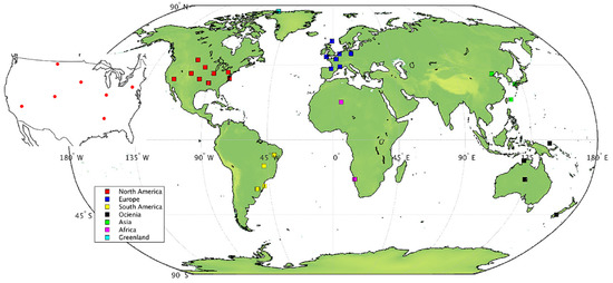
Figure 1.
SURFRAD (circles) and BSRN (squares) sites used for validation.
2.3. Algorithm Framework
The algorithm firstly optimizes surface and atmospheric parameters from TOA reflectance and subsequently estimates ISR. Then we used the Wang and Liang method [49] to calculate daily integrated ISR from VIIRS observations. We validated the results against field measurements from seven SURFRAD sites and 33 BSRN sites globally. There are several major improvements over the earlier version of the algorithm, including (1) integrated look-up table and optimization framework, (2) calculation of net shortwave radiation as well, (3) adding the estimation of daily values, and (4) extensive global validation. We produced global daily integrated ISR maps on 1 January, April, July, and October 2018 as examples.
Figure 2 illustrates the framework of the algorithm. An optimization method has been used [52,54] to estimate surface reflectance and broadband albedo. In our previous research, we developed a similar approach for incident shortwave radiation estimation from MODIS data by revising the cost function considering both satellite observations and optional constraints, including aerosol optical depth (AOD), cloud optical depth (COD), surface reflectance products, and albedo climatology [51]. In this study, we adapted the algorithm for the estimation of ISR from VIIRS data by revising the band configuration and the spectrum of radiation transfer simulation. An assumption is made here that the surface reflectance is invariant during a short period (8 days in this research). Under cloudy sky conditions, we used the surface reflectance calculated by the nearest previous clear observations as surface input. The COD can then be optimized using radiative transfer models.
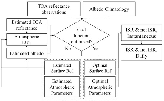
Figure 2.
Framework of the ISR estimation algorithm.
In this study, atmospheric optical parameters such as spherical albedo, atmospheric downward/upward transmittance, and path reflectance are required to calculate the cost function. We used libRadtran [55] to simulate the parameters.
We used surface and atmospheric parameters to implement a forward simulation of TOA reflectance using the radiative transfer model. The cost function is based on the difference between simulated and observed TOA reflectance (Equations (1)–(3)):
Here, and refer to satellite-observed TOA reflectance and forward-simulated TOA reflectance from the radiative transfer model. and are the calculated albedo and the albedo climatology, respectively. and are the parameters to be optimized under clear and cloudy sky cases, respectively. O and B are the error matrices for the TOA reflectance and the climatology, respectively. The albedo climatology covariance matrix B is determined from the multiyear satellite albedo climatology uncertainty, while the TOA reflectance covariance matrix O is calculated from the narrowband albedo’s contribution to the broadband albedo and the spectral reflectance magnitude. Jc is a punishment component and set to a 100 if the TOA reflectance is an invalid value (negative or greater than one). The shuffled complex evolution (SCE) method [56] was used to search for the optimum.
When the surface and atmospheric parameters reach an optimum, ISR and NSR are then calculated using a radiative transfer model according to Equations (4)–(6):
Here, is the radiation without any contribution from the surface, while and denote the direct and diffuse parts, respectively. is the surface reflectance, is the spherical albedo, is the cosine of the solar zenith angle, is the extraterrestrial solar radiation, and is the total transmittance. For each combination of geometry and optical depth, the , , and were pre-calculated by radiative transfer simulation in the ISR spectrum range and stored in a look-up table. denotes the land surface broadband albedo, and denote surface ISR and NSR, respectively.
Equations (4)–(6) are based on instantaneous observations. The daily ISR were then estimated using the LUT-based algorithm by Wang et al. [57]. We calculated ISR every 30 min according to the interpolation algorithm. Then, we calculated the average ISR for each day.
2.4. Atmospheric Look-up Tables Improvements
Atmospheric optical parameters such as spherical albedo, atmospheric downward/upward transmittance, and path reflectance are required to implement a forward simulation. To make the algorithm more efficient, all the parameters were pre-calculated in representative geometries and atmospheric conditions (AOD, cloud optical depth [COD] cloud effective radius [CER]). LibRadtran [55] software was used for the generation of the LUT. The following values were used as entries in the radiative transfer simulations: solar zenith angle (0°–80°, at 10° intervals), viewing zenith angle (0°–80°, at 20° intervals), relative azimuth angle (0°–180°, at 30° intervals), AOD at 550 nm (0.01, 0.025, 0.05, 0.1, 0.2, 0.3, 0.4, 0.5, 0.6, 0.7, 0.8, 0.9, 1.0), surface elevation (0, 1, 2, 3 4, 5 km), and water vapor (0, 15, 30, 45, 60, 75, 90, 105 mm). COD (1, 3, 5, 10, 20, 40, 60, 80) and CER (3, 6, 9, 12 um) are set for water cloud while CER (20, 30, 40, 50, 60, 70, 80 um) are set for ice cloud.
We used the continental-clean model to estimate ISR. For each specific solar/viewing geometry and atmospheric parameter (AOD at 550 nm for clear-sky conditions, COD and CER for cloudy-sky conditions), radiative transfer simulations generated path reflectance, upward/downward transmittances, and spherical albedo for each of the seven VIIRS bands. We used actual site elevation to estimate ISR at the SURFRAD and BSRN sites, and the Global 30 Arc-Second Elevation (GTOPO30) [58,59] for the global ISR map. With the atmospheric LUT, we calculated the surface broadband albedo and atmospheric index (AOD for clear-sky conditions, COD and CER for cloudy-sky conditions) from the optimization process. For cloudy-sky cases, each observation was optimized using both the water and ice cloud LUTs, of which the one with a smaller cost function result was chosen as the result. ISR could then be calculated under certain geometries using the surface radiation LUT. In this paper, we calculated the ISR for the spectral range of 280–2800 nm to match the field measurements.
2.5. Improvement of the Optimization Framework
In the previous MODIS algorithm, most of the unknown variables in the optimization process were surface parameters while only one was for the atmospheric condition (AOD/COD). We prioritized the unknown variables in this research to increase more atmospheric parameters.
The influence of ISR is much more associated with the atmospheric conditions, especially the cloud conditions. Surface parameters also count for multiple scattering which also contributes to the ISR. In this research, we tried to minimize the unknown surface variables to increase both the efficiency and accuracy of the model.
We used principal component analysis (PCA) to analyze the surface spectral reflectance of the nine VIIRS bands using the data from all the site measurements extracted from reflectance products. Results show that the first two components explain more than 98 percent of the variations. In the updated framework, we only use two free variables for the surface condition, which reduce the total unknown variables to three in clear-sky conditions and four in cloudy-sky conditions.
The PCA could increase the efficiency with low errors introduced. The ISR is mainly determined by the path flux (the first component in Equation (4)) and the multiple scattering part (the second component in Equation (4)). The albedo climatology ] in Equation (1) constrains the surface reflectance and albedo error. Over dark surfaces, such as forests, the multiple scattering part is minimal in determining the overall ISR due to the low surface albedo. On the other hand, over bright surfaces such as deserts, the principal components could explain much of the overall variations due to relatively simple surface conditions.
Figure 3a illustrates the radiative transfer simulated maximum error over dark and bright surfaces with the first two components at nadir (solar zenith angle = 0). The maximum possible differences at nadir are calculated under different visibility conditions. The error is more massive when the cloud is dense (optical depth greater than 80), and when dense aerosol (optical depth between 1 ~ 2, usually results from a mixture of aerosol and cloud). In all cases, the induced error is less than 1.6 W/m2. Figure 3b,c show the original spectral reflectance and the PCs from multiple sites over bright surfaces. The PC1 explains the variation for spectral bands at a shorter wavelength (<1000 nm), while the PC2 explains the other bands.
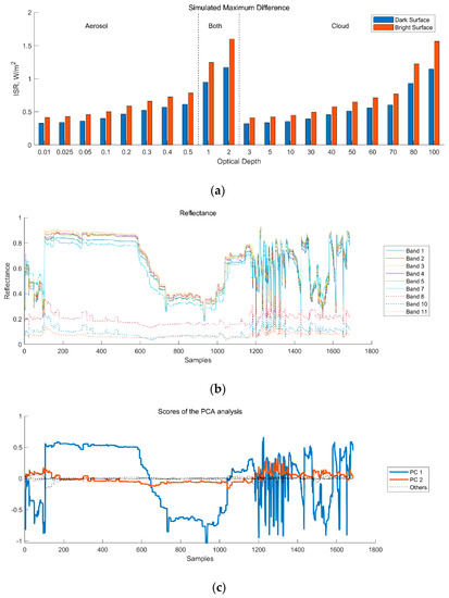
Figure 3.
Principal component analysis of the nine VIIRS spectral reflectance: (a) Simulated maximum differences in ISR estimation over dark and bright surfaces with the first two components; (b) Original spectral reflectance over bright surfaces; (c) Scores of PCA.
3. Results over SURFRAD Sites
3.1. Validation Results of Instantaneous ISR
The validation results of instantaneous ISR are shown in Figure 4 and Table 3. The ISR RMSE ranges from 75.32 W/m2 to 94.66 W/m2 at the different sites while the bias ranges from −29.36 W/m2 to 9.21 W/m2. The overall RMSE and bias are 83.76 W/m2 and −3.49 W/m2, respectively. RMSEOrigin denotes the results from the original optimization framework without the improvements. The updated algorithm provides accuracy improvement at most of the SURFRAD sites and the overall result.
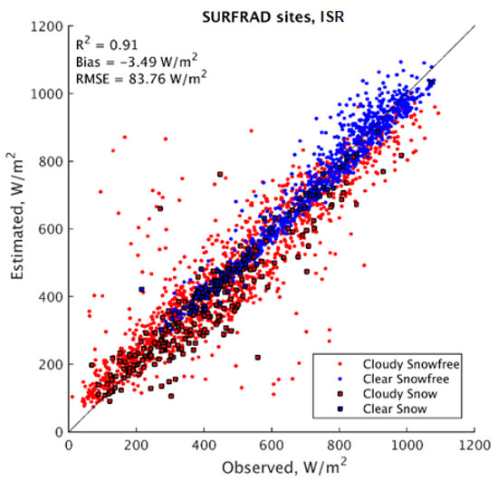
Figure 4.
Validation results of instantaneous ISR at SURFRAD sites. Circles: Snow−free surface, Squares: Snow surface; Red: Cloudy−sky cases, Blue: Clear−sky cases.
Table 3.
Validation results of instantaneous ISR at SURFRAD sites.
3.2. Validation Results of Instantaneous NSR
The validation results of instantaneous NSR are shown in Figure 5 and Table 4. The RMSE ranges from 56.8 W/m2 to 80.87 W/m2 at the different sites while the bias ranges from −20.48 W/m2 to 14.6 W/m2. The overall RMSE and bias are 66.80 W/m2 and 0.62 W/m2, respectively.
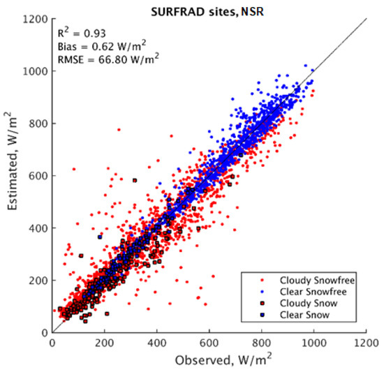
Figure 5.
Validation results of instantaneous NSR at SURFRAD sites. Circles: Snow−free surface, Squares: Snow surface; Red: Cloudy−sky cases, Blue: Clear−sky cases.
Table 4.
Validation results of instantaneous NSR at SURFRAD sites.
3.3. Validation Results of Daily ISR
The validation results of daily ISR are shown in Figure 6 and Table 5. The ISR RMSE ranges from 24.40 W/m2 to 34.11 W/m2 at the different sites while the bias ranges from −8.60 to 10.59 W/m2. The overall daily RMSE and bias are 27.78 W/m2 and −0.16 W/m2, respectively.
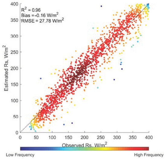
Figure 6.
Validation results of daily ISR at SURFRAD sites.
Table 5.
Validation results of daily ISR at SURFRAD sites.
3.4. Validation Results of Daily NSR
The validation results of daily NSR are shown in Figure 7 and Table 6. The RMSE ranges from 18.07 W/m2 to 30.31 W/m2 at the different sites while the bias ranges from –0.99 W/m2 to 4.51 W/m2. The overall RMSE and bias are 23.51 W/m2 and 2.66 W/m2, respectively.
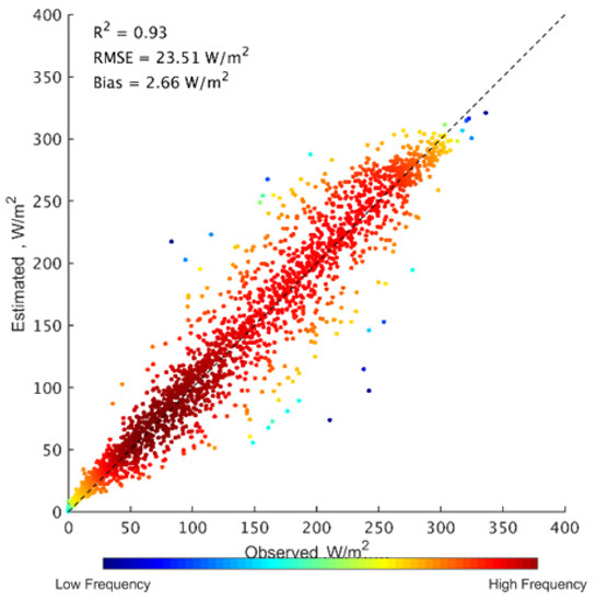
Figure 7.
Validation results of daily NSR at SURFRAD sites.
Table 6.
Validation results of daily NSR at SURFRAD sites.
4. Results over BSRN sites
4.1. Validation Results of Instantaneous ISR
The validation results of instantaneous ISR are shown in Figure 8, Table 7 and Table 8. The ISR RMSE in North America ranges from 95.41 W/m2 to 127.65 W/m2 at the different sites while the bias ranges from −26.89 W/m2 to −1.55 W/m2. The overall RMSE and bias are 112.39 W/m2 and −14.05 W/m2, respectively. The RMSE at BSRN sites is generally higher than that at SURFRAD sites even they are close to each other.
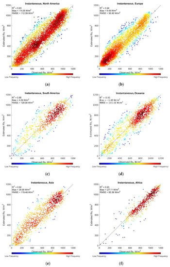
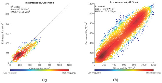
Figure 8.
Validation results of instantaneous ISR in different areas: (a) North America; (b) Europe; (c) South America; (d) Oceania; (e) Asia; (f) Africa; (g) Greenland; (h) All.
Table 7.
Validation results of instantaneous ISR at all BSRN sites.
Table 8.
Validation results of instantaneous ISR in different areas.
The ISR RMSE in Europe ranges from 86.72 W/m2 to 106.09 W/m2 at the different sites while the bias ranges from −26.89 W/m2 to −1.55 W/m2. The overall RMSE and bias are 95.90 W/m2 and 9.48 W/m2, respectively.
The ISR RMSE in South America ranges from 111.01 W/m2 to 156.99 W/m2 at the different sites while the bias ranges from −10.06 W/m2 to 26.04 W/m2. The overall RMSE and bias are 129.00 W/m2 and 4.29 W/m2, respectively.
The ISR RMSE in Oceania ranges from 89.48 W/m2 to 147.77 W/m2 at the different sites while the bias ranges from −35.15 W/m2 to 47.89 W/m2. The overall RMSE and bias are 115.16 W/m2 and −1.49 W/m2, respectively.
The ISR RMSE in Asia ranges from 109.98 W/m2 to 132.63 W/m2 at the different sites while the bias ranges from 29.55 W/m2 to 43.23 W/m2. The overall RMSE and bias are 119.48 W/m2 and 34.09 W/m2, respectively.
The ISR RMSE in Africa ranges from 60.2 W/m2 to 109.39 W/m2 at the different sites while the bias ranges from −53.23 W/m2 to −9.8 W/m2. The overall RMSE and bias are 83.36 W/m2 and −27.11 W/m2, respectively.
There is only one site located in this Greenland area. The RMSE and bias are 74.28 W/m2 and −40.71 W/m2, respectively.
The validation results of instantaneous ISR are shown in Figure 8, Table 7 and Table 8. The ISR RMSE in each area ranges from 83.36 W/m2 to 129 W/m2 at the different sites while the bias ranges from −40.71 W/m2 to 9.48 W/m2. South America sites have the largest overall RMSE as there is more cloud in this area. Greenland site has the smallest RMSE due to the high latitude and the low absolute value of ISR. The overall RMSE and bias are 105.87 W/m2 and −3.79 W/m2, respectively.
4.2. Validation Results of Daily ISR
The validation results of daily ISR are shown in Figure 9, Table 9 and Table 10. The ISR in North America RMSE ranges from 26.41 W/m2 to 39.96 W/m2 at the different sites while the bias ranges from −8.89 W/m2 to 2.2 W/m2. The overall RMSE and bias are 34.57 W/m2 and −3.08 W/m2, respectively.
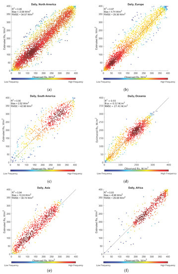
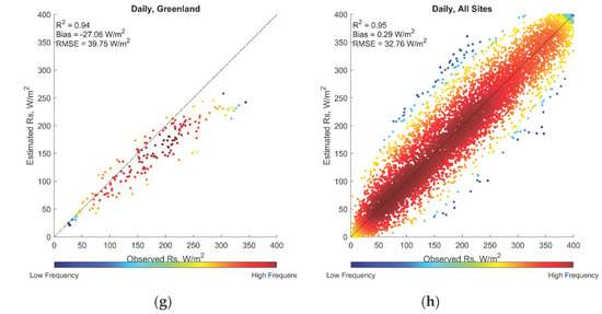
Figure 9.
Validation results of daily ISR in different areas: (a) North America; (b) Europe; (c) South America; (d) Oceania; (e) Asia; (f) Africa; (g) Greenland; (h) All.
Table 9.
Validation results of daily ISR at all BSRN sites.
Table 10.
Validation results of daily ISR in different areas.
The ISR in Europe RMSE ranges from 25.4 W/m2 to 33.07 W/m2 at the different sites while the bias ranges from −0.35 W/m2 to 6.97 W/m2. The overall RMSE and bias are 29.36 W/m2 and 4.74 W/m2, respectively.
The ISR RMSE in South America ranges from 34.13 W/m2 to 55.09 W/m2 at the different sites while the bias ranges from −3.05 W/m2 to 9.4 W/m2. The overall RMSE and bias are 42.98 W/m2 and 2.52 W/m2, respectively.
The ISR RMSE in Oceania ranges from 17.41 W/m2 to 34.63 W/m2 at the different sites while the bias ranges from −7.44 W/m2 to 11.02 W/m2. The overall RMSE and bias are 27.41 W/m2 and 0.52 W/m2, respectively.
The ISR RMSE in Asia ranges from 27.8 W/m2 to 34.04 W/m2 at the different sites while the bias ranges from 7.78 W/m2 to 14.53 W/m2. The overall RMSE and bias are 30.74 W/m2 and 10.24 W/m2, respectively.
The ISR RMSE in Africa ranges from 18.3 W/m2 to 40.56 W/m2 at the different sites while the bias ranges from −17.53 W/m2 to−3.52 W/m2. The overall RMSE and bias are 29.08 W/m2 and −8.98 W/m2, respectively.
The RMSE and bias in the Greenland area site are 39.75 W/m2 and −27.06 W/m2, respectively.
5. Discussion and Conclusions
5.1. Spatial and Temporal Analysis
Figure 10 shows the seasonal variation of relative biases and RMSEs over the different regions. Most of the northern hemisphere sites, including North America, Europe, and Asia sites overestimate ISR in summer and underestimate in winter. Tropical and sub-tropical sites, including South America and Oceania sites, show no significant seasonal changes on biases. Greenland site shows significant underestimation as the algorithm underestimates the cloud optical depth due to the snow land surface, which should be improved in future research. Most of the sites have larger relative RMSE in winter, as the absolute ISR values are usually smaller in winter.
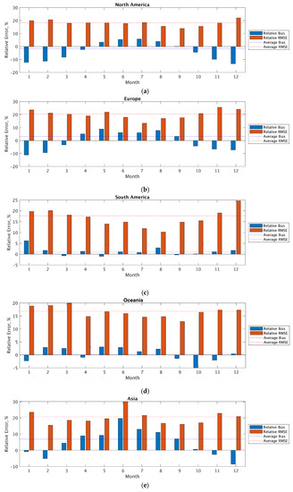
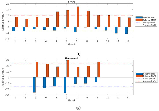
Figure 10.
Seasonal analysis of daily mean ISR: (a) North America; (b) Europe; (c) South America; (d) Oceania; (e) Asia; (f) Africa; (g) Greenland.
Figure 11 and Figure 12 show the spatial patterns of the validation results for instantaneous and daily ISR, respectively. Red circles denote sites with positive biases while blue circles denote sites with negative biases. The larger the diameters of the circles, the larger the RMSEs are and vice versa. Overall, sites located in lower latitudes and located in islands have larger RMSEs compared to other sites. The algorithm tends to underestimate ISR over North America and overestimate ISR over Europe and Asia. Figure 13. shows the VIIRS daily ISR map on 1 Jan. 2018.
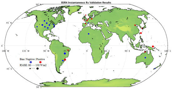
Figure 11.
Validation results of instantaneous ISR: red circles denote sites with positive biases while blue circles denote sites with negative biases, the diameters of the circles represent the RMSEs.
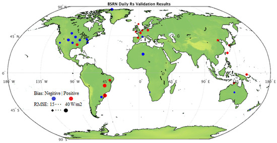
Figure 12.
Validation results of daily ISR: red circles denote sites with positive biases while blue circles denote sites with negative biases, the diameters of the circles represent the RMSEs.
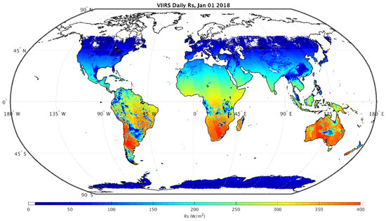
Figure 13.
VIIRS daily ISR on 1 Jan. 2018.
5.2. Discussion
The PCA performed to the surface reflectance could reduce the optimization framework’s unknown variables, providing a significant improvement in efficiency and slight inaccuracy. Many previous studies used surface reflectance from single or multiple spectral bands to estimate surface ISR. Traditional single-band LUT algorithms tend to assume a single condition that the band used (often the blue band) itself can represent the surface condition and determine the atmosphere’s clearness. On the other hand, the optimization algorithm using all shortwave spectral bands is time-consuming. The PCA can extract critical information for the surface condition. Apart from improving the efficiency, the approach can also improve the accuracy slightly, as fewer free variables bring less uncertainty to the optimization process.
The most significant improvement is at the Table Mountain site at Boulder (CO, USA). The cloud condition in the mountainous area here is the most complicated among the SURFRAD sites. Overall, sites with dark surfaces have slight improvement while not at the sites with bright surfaces, such as Desert Rock. Further improvements are required to apply this algorithm over the bright surfaces.
Boundaries between different orbits over southern Africa and Australia in the global daily map indicate that estimating daily averaged ISR from instantaneous observations is difficult. Further work is required in generating global operational products.
5.3. Conclusions
This research modified the optimization based ISR estimation algorithm and applied it to VIIRS data. We validated instantaneous and daily ISR globally over SURFRAD and BSRN sites and performed the spatial and temporal analysis.
The ISR products are still not available from VIIRS observation. Here we present a framework for estimating instantaneous and daily ISR products from VIIRS observation. The algorithm was used for MODIS instantaneous ISR estimation. We adapted and extended the algorithm for VIIRS data. We validated the results at seven SURFRAD and 33 BSRN sites. The RMSE over SURFRAD sites were 83.76 W/m2 for instantaneous ISR and 66.80 W/m2 and instantaneous NSR. Daily results showed 27.78 W/m2 and 23.51 W/m2 for ISR and NSR, respectively. Validation results at BSRN sites present RMSEs of 105.87 W/m2 for instantaneous ISR and 32.76 W/m2 for daily ISR.
The algorithm can estimate instantaneous, and daily ISR from VIIRS data at a similar or better accuracy than existing products and can provide much higher spatial resolution. However, the optimization-based method generated greater uncertainty compared to that of the previous MODIS algorithm, mainly because the latter combines observations from the local morning and local afternoon. Further research can be undertaken to improve the cost function and the optimization framework in the case of a lack of high-level products as constraints and apply the algorithm in the global operational production of 375/750 m resolution.
Author Contributions
Conceptualization Y.Z. and S.L.; investigation Y.Z.; writing Y.Z.; review and editing S.L., T.H., D.W. and Y.Y. All authors have read and agreed to the published version of the manuscript.
Funding
This research was supported in part by the National Key Research and Development Program of China (NO.2016YFA0600103), in part by the National Natural Science Foundation of China Grant 42090012, in part by the China Postdoctoral Science Foundation Grant (2019M652707), in part by the National Aeronautics and Space Administration (NASA) under grant 80NSSC18K0620 and in part by NOAA GOES-R funding through the University of Maryland. We thank Microsoft AI or Earth for providing cloud computing resources.
Acknowledgments
We gratefully acknowledge the VIIRS team for providing access to the land and atmosphere products online. We also thank the SURFRAD and BSRN teams for providing and maintaining all the data sets used for the validation in this study.
Conflicts of Interest
The authors declare no conflict of interest.
References
- Liang, S.; Wang, K.; Zhang, X.; Wild, M. Review on Estimation of Land Surface Radiation and Energy Budgets from Ground Measurement, Remote Sensing and Model Simulations. IEEE J. Sel. Top. Appl. Earth Obs. Remote Sens. 2010, 3, 225–240. [Google Scholar] [CrossRef]
- Jiang, B.; Zhang, Y.; Liang, S.; Wohlfahrt, G.; Arain, A.; Cescatti, A.; Georgiadis, T.; Jia, K.; Kiely, G.; Lund, M.; et al. Empirical estimation of daytime net radiation from shortwave radiation and ancillary information. Agric. For. Meteorol. 2015, 211, 23–36. [Google Scholar] [CrossRef]
- Jiang, B.; Zhang, Y.; Liang, S.; Zhang, X.; Xiao, Z. Surface Daytime Net Radiation Estimation Using Artificial Neural Networks. Remote Sens. 2014, 6, 11031–11050. [Google Scholar] [CrossRef]
- Huang, G.; Li, Z.; Li, X.; Liang, S.; Yang, K.; Wang, D.; Zhang, Y. Estimating surface solar irradiance from satellites: Past, present, and future perspectives. Remote Sens. Environ. 2019, 233, 111371. [Google Scholar] [CrossRef]
- Liang, S. Quantitative Remote Sensing of Land Surfaces; Wiley-Interscience: Hoboken, NJ, USA, 2004; p. xxvi. [Google Scholar]
- Liang, S.; Wang, J. Advanced Remote Sensing: Terrestrial Information Extraction and Applications; Academic Press: Cambridge, MA, USA, 2019. [Google Scholar]
- Augustine, J.A.; DeLuisi, J.J.; Long, C.N. SURFRAD—A National Surface Radiation Budget Network for Atmospheric Research. Bull. Am. Meteorol. Soc. 2000, 81, 2341–2357. [Google Scholar] [CrossRef]
- Kobayashi, S.; Ota, Y.; Harada, Y.; Ebita, A.; Moriya, M.; Onoda, H.; Onogi, K.; Kamahori, H.; Kobayashi, C.; Endo, H.; et al. The JRA-55 Reanalysis: General Specifications and Basic Characteristics. J. Meteorol. Soc. Jpn. 2015, 93, 5–48. [Google Scholar] [CrossRef]
- Hersbach, H.; Bell, B.; Berrisford, P.; Hirahara, S.; Horányi, A.; Muñoz-Sabater, J.; Nicolas, J.; Peubey, C.; Radu, R.; Schepers, D. The ERA5 global reanalysis. Q. J. R. Meteorol. Soc. 2020, 146, 1999–2049. [Google Scholar] [CrossRef]
- Rienecker, M.M.; Suarez, M.J.; Gelaro, R.; Todling, R.; Bacmeister, J.; Liu, E.; Bosilovich, M.G.; Schubert, S.D.; Takacs, L.; Kim, G.-K.; et al. MERRA: NASA’s Modern-Era Retrospective Analysis for Research and Applications. J. Clim. 2011, 24, 3624–3648. [Google Scholar] [CrossRef]
- Kistler, R.; Kalnay, E.; Collins, W.; Saha, S.; White, G.; Woollen, J.; Chelliah, M.; Ebisuzaki, W.; Kanamitsu, M.; Kousky, V.; et al. The NCEP-NCAR 50-year reanalysis: Monthly means CD-ROM and documentation. Bull. Am. Meteorol. Soc. 2001, 82, 247–267. [Google Scholar] [CrossRef]
- Kalnay, E.; Kanamitsu, M.; Kistler, R.; Collins, W.; Deaven, D.; Gandin, L.; Iredell, M.; Saha, S.; White, G.; Woollen, J.; et al. The NCEP/NCAR 40-year reanalysis project. Bull. Am. Meteorol. Soc. 1996, 77, 437471. [Google Scholar] [CrossRef]
- Saha, S.; Moorthi, S.; Pan, H.-L.; Wu, X.; Wang, J.; Nadiga, S.; Tripp, P.; Kistler, R.; Woollen, J.; Behringer, D.; et al. The NCEP Climate Forecast System Reanalysis. Bull. Am. Meteorol. Soc. 2010, 91, 1015–1058. [Google Scholar] [CrossRef]
- Wielicki, B.A.; Barkstrom, B.R.; Harrison, E.F.; Lee, R.B.; Smith, G.L.; Cooper, J.E. Clouds and the earth’s radiant energy system (CERES): An earth observing system experiment. Bull. Am. Meteorol. Soc. 1996, 77, 853–868. [Google Scholar] [CrossRef]
- Zhang, Y.; Rossow, W.B.; Lacis, A.A.; Oinas, V.; Mishchenko, M.I. Calculation of radiative fluxes from the surface to top of atmosphere based on ISCCP and other global data sets: Refinements of the radiative transfer model and the input data. J. Geophys. Res.-Atmos. 2004, 109. [Google Scholar] [CrossRef]
- Pinker, R.T.; Laszlo, I. Modeling Surface Solar Irradiance for Satellite Applications on a Global Scale. J. Appl. Meteorol. 1992, 31, 194–211. [Google Scholar] [CrossRef]
- Wang, D.; Liang, S.; Zhang, Y.; Gao, X.; Brown, M.G.L.; Jia, A. A New Set of MODIS Land Products (MCD18): Downward Shortwave Radiation and Photosynthetically Active Radiation. Remote Sens. 2020, 12, 168. [Google Scholar] [CrossRef]
- Liang, S.; Cheng, J.; Jia, K.; Jiang, B.; Liu, Q.; Xiao, Z.; Yao, Y.; Yuan, W.; Zhang, X.; Zhao, X.; et al. The Global LAnd Surface Satellite (GLASS) product suite. Bull. Am. Meteorol. Soc. 2020, 1–37. [Google Scholar] [CrossRef]
- Müller, R.; Matsoukas, C.; Gratzki, A.; Behr, H.; Hollmann, R. The CM-SAF operational scheme for the satellite based retrieval of solar surface irradiance—A LUT based eigenvector hybrid approach. Remote Sens. Environ. 2009, 113, 1012–1024. [Google Scholar] [CrossRef]
- Gui, S.; Liang, S.; Wang, K.; Li, L.; Zhang, A.X. Assessment of Three Satellite-Estimated Land Surface Downwelling Shortwave Irradiance Data Sets. IEEE Geosci. Remote Sens. Lett. 2010, 7, 776–780. [Google Scholar] [CrossRef]
- Zhang, X.; Liang, S.; Wild, M.; Jiang, B. Analysis of surface incident shortwave radiation from four satellite products. Remote Sens. Environ. 2015, 165, 186–202. [Google Scholar] [CrossRef]
- Jia, B.; Xie, Z.; Dai, A.; Shi, C.; Chen, F. Evaluation of satellite and reanalysis products of downward surface solar radiation over East Asia: Spatial and seasonal variations. J. Geophys. Res. Atmos. 2013, 118, 3431–3446. [Google Scholar] [CrossRef]
- Zhang, X.; Liang, S.; Wang, G.; Yao, Y.; Jiang, B.; Cheng, J. Evaluation of the Reanalysis Surface Incident Shortwave Radiation Products from NCEP, ECMWF, GSFC, and JMA Using Satellite and Surface Observations. Remote Sens. 2016, 8, 225. [Google Scholar] [CrossRef]
- Bisht, G.; Bras, R.L. Estimation of net radiation from the MODIS data under all sky conditions: Southern Great Plains case study. Remote Sens. Environ. 2010, 114, 1522–1534. [Google Scholar] [CrossRef]
- Forman, B.A.; Margulis, S.A. High-resolution satellite-based cloud-coupled estimates of total downwelling surface radiation for hydrologic modelling applications. Hydrol. Earth Syst. Sci. 2009, 13, 969–986. [Google Scholar] [CrossRef]
- Qin, J.; Tang, W.; Yang, K.; Lu, N.; Niu, X.; Liang, S. An efficient physically based parameterization to derive surface solar irradiance based on satellite atmospheric products. J. Geophys. Res. Atmos. 2015, 120, 4975–4988. [Google Scholar] [CrossRef]
- Tang, W.; Qin, J.; Yang, K.; Liu, S.; Lu, N.; Niu, X. Retrieving high-resolution surface solar radiation with cloud parameters derived by combining MODIS and MTSAT data. Atmos. Chem. Phys. Discuss. 2016, 16, 2543–2557. [Google Scholar] [CrossRef]
- Van Laake, P.E.; Sanchez-Azofeifa, G. Simplified atmospheric radiative transfer modelling for estimating incident PAR using MODIS atmosphere products. Remote Sens. Environ. 2004, 91, 98–113. [Google Scholar] [CrossRef]
- Huang, G.; Liang, S.; Lu, N.; Ma, M.; Wang, D. Toward a Broadband Parameterization Scheme for Estimating Surface Solar Irradiance: Development and Preliminary Results on MODIS Products. J. Geophys. Res. Atmos. 2018, 123. [Google Scholar] [CrossRef]
- Huang, G.; Li, X.; Ma, M.; Li, H.; Huang, C. High resolution surface radiation products for studies of regional energy, hydrologic and ecological processes over Heihe river basin, northwest China. Agric. For. Meteorol. 2016, 230, 67–78. [Google Scholar] [CrossRef]
- Huang, G.; Ma, M.; Liang, S.; Liu, S.M.; Li, X. A LUT-based approach to estimate surface solar irradiance by combining MODIS and MTSAT data. J. Geophys. Res. Space Phys. 2011, 116. [Google Scholar] [CrossRef]
- Liang, S.; Zheng, T.; Liu, R.; Fang, H.; Tsay, S.-C.; Running, S. Estimation of incident photosynthetically active radiation from Moderate Resolution Imaging Spectrometer data. J. Geophys. Res. Space Phys. 2006, 111, 111. [Google Scholar] [CrossRef]
- Zhang, X.; Liang, S.; Zhou, G.; Wu, H.; Zhao, X. Generating Global LAnd Surface Satellite incident shortwave radiation and photosynthetically active radiation products from multiple satellite data. Remote Sens. Environ. 2014, 152, 318–332. [Google Scholar] [CrossRef]
- Pinker, R.T.; Tarpley, J.D.; Laszlo, I.; Mitchell, K.E.; Houser, P.R.; Wood, E.F.; Schaake, J.C.; Robock, A.; Lohmann, D.; Cosgrove, B.A.; et al. Surface radiation budgets in support of the GEWEX Continental-Scale International Project (GCIP) and the GEWEX Americas Prediction Project (GAPP), including the North American Land Data Assimilation System (NLDAS) project. J. Geophys. Res. Res.-Atmos. 2003, 108. [Google Scholar] [CrossRef]
- Aguiar, L.M.; Pereira, B.; David, M.; Díaz, F.; Lauret, P. Use of satellite data to improve solar radiation forecasting with Bayesian Artificial Neural Networks. Sol. Energy 2015, 122, 1309–1324. [Google Scholar] [CrossRef]
- Akarslan, E.; Hocaoglu, F.O. A novel adaptive approach for hourly solar radiation forecasting. Renew. Energy 2016, 87, 628–633. [Google Scholar] [CrossRef]
- Akarslan, E.; Hocaoğlu, F.O.; Edizkan, R. A novel M-D (multi-dimensional) linear prediction filter approach for hourly solar radiation forecasting. Energy 2014, 73, 978–986. [Google Scholar] [CrossRef]
- Janjai, S.; Pankaew, P.; Laksanaboonsong, J. A model for calculating hourly global solar radiation from satellite data in the tropics. Appl. Energy 2009, 86, 1450–1457. [Google Scholar] [CrossRef]
- Mefti, A.; Adane, A.-E.-H.; Bouroubi, M. Satellite approach based on cloud cover classification: Estimation of hourly global solar radiation from meteosat images. Energy Convers. Manag. 2008, 49, 652–659. [Google Scholar] [CrossRef]
- Yang, L.; Zhang, X.; Liang, S.; Yao, Y.; Jia, K.; Jia, A. Estimating Surface Downward Shortwave Radiation over China Based on the Gradient Boosting Decision Tree Method. Remote Sens. 2018, 10, 185. [Google Scholar] [CrossRef]
- Ma, H.; Liang, S.; Shi, H.; Zhang, Y. An Optimization Approach for Estimating Multiple Land Surface and Atmospheric Variables from the Geostationary Advanced Himawari Imager Top-of-Atmosphere Observations. IEEE Trans. Geosci. Remote Sens. 2020, 1–21. [Google Scholar] [CrossRef]
- Ma, H.; Liang, S.; Xiao, Z.; Wang, D. Simultaneous Estimation of Multiple Land-Surface Parameters from VIIRS Optical-Thermal Data. IEEE Geosci. Remote Sens. Lett. 2017, 15, 156–160. [Google Scholar] [CrossRef]
- Ma, H.; Liang, S.; Xiao, Z.; Shi, H. Simultaneous inversion of multiple land surface parameters from MODIS optical–thermal observations. ISPRS J. Photogramm. Remote Sens. 2017, 128, 240–254. [Google Scholar] [CrossRef]
- He, T.; Liang, S.; Wang, D.; Shi, Q.; Goulden, M.L. Estimation of high-resolution land surface net shortwave radiation from AVIRIS data: Algorithm development and preliminary results. Remote Sens. Environ. 2015, 167, 20–30. [Google Scholar] [CrossRef]
- Wang, D.; Liang, S.; He, T.; Shi, Q. Estimating clear-sky all-wave net radiation from combined visible and shortwave infrared (VSWIR) and thermal infrared (TIR) remote sensing data. Remote Sens. Environ. 2015, 167, 31–39. [Google Scholar] [CrossRef]
- Kim, H.-Y.; Liang, S. Development of a hybrid method for estimating land surface shortwave net radiation from MODIS data. Remote Sens. Environ. 2010, 114, 2393–2402. [Google Scholar] [CrossRef]
- Wang, D.; Liang, S.; He, T. Mapping high-resolution surface shortwave net radiation from Landsat data. IEEE Geosci. Remote Sens. Lett. 2013, 11, 459–463. [Google Scholar] [CrossRef]
- Wang, T.; Yan, G.; Chen, L. Consistent retrieval methods to estimate land surface shortwave and longwave radiative flux components under clear-sky conditions. Remote Sens. Environ. 2012, 124, 61–71. [Google Scholar] [CrossRef]
- Wang, D.; Liang, S.; He, T.; Shi, Q. Estimation of daily surface shortwave net radiation from the combined MODIS data. IEEE Trans. Geosci. Remote Sens. 2015, 53, 5519–5529. [Google Scholar] [CrossRef]
- Mateos, D.; Bilbao, J.; Kudish, A.; Parisi, A.V.; Carbajal, G.; Di Sarra, A.; Román, R.; De Migue, A. Validation of OMI satellite erythemal daily dose retrievals using ground-based measurements from fourteen stations. Remote Sens. Environ. 2013, 128, 1–10. [Google Scholar] [CrossRef]
- Zhang, Y.; He, T.; Liang, S.; Wang, D.; Yu, Y. Estimation of all-sky instantaneous surface incident shortwave radiation from Moderate Resolution Imaging Spectroradiometer data using optimization method. Remote Sens. Environ. 2018, 209, 468–479. [Google Scholar] [CrossRef]
- He, T.; Liang, S.; Wang, D.; Wu, H.; Yu, Y.; Wang, J. Estimation of surface albedo and directional reflectance from Moderate Resolution Imaging Spectroradiometer (MODIS) observations. Remote Sens. Environ. 2012, 119, 286–300. [Google Scholar] [CrossRef]
- Huang, G.; Li, X.; Huang, C.; Liu, S.M.; Ma, Y.; Chen, H. Representativeness errors of point-scale ground-based solar radiation measurements in the validation of remote sensing products. Remote Sens. Environ. 2016, 181, 198–206. [Google Scholar] [CrossRef]
- He, T.; Zhang, Y.; Liang, S.; Yu, Y.; Wang, D. Developing Land Surface Directional Reflectance and Albedo Products from Geostationary GOES-R and Himawari Data: Theoretical Basis, Operational Implementation, and Validation. Remote Sens. 2019, 11, 2655. [Google Scholar] [CrossRef]
- Mayer, B.; Kylling, A. Technical note: The libRadtran software package for radiative transfer calculations—Description and examples of use. Atmos. Chem. Phys. Discuss. 2005, 5, 1855–1877. [Google Scholar] [CrossRef]
- Duan, Q.; Sorooshian, S.; Gupta, V.K. Optimal use of the SCE-UA global optimization method for calibrating watershed models. J. Hydrol. 1994, 158, 265–284. [Google Scholar] [CrossRef]
- Wang, D.; Liang, S.; Liu, R.; Zheng, T. Estimation of daily-integrated PAR from sparse satellite observations: Comparison of temporal scaling methods. Int. J. Remote Sens. 2010, 31, 1661–1677. [Google Scholar] [CrossRef]
- Danielson, J.J.; Gesch, D.B. Global Multi-Resolution Terrain Elevation Data 2010 (GMTED2010); US Department of the Interior, US Geological Survey: Reston, VA, USA, 2011.
- Gesch, D.B.; Verdin, K.L.; Greenlee, S.K. New land surface digital elevation model covers the Earth. EOS Trans. Am. Geophys. Union 1999, 80, 69–70. [Google Scholar] [CrossRef]
Publisher’s Note: MDPI stays neutral with regard to jurisdictional claims in published maps and institutional affiliations. |
© 2020 by the authors. Licensee MDPI, Basel, Switzerland. This article is an open access article distributed under the terms and conditions of the Creative Commons Attribution (CC BY) license (http://creativecommons.org/licenses/by/4.0/).