Detection of Two Different Grapevine Yellows in Vitis vinifera Using Hyperspectral Imaging

Abstract

Grapevine yellows (GY) are serious phytoplasma-caused diseases affecting viticultural areas worldwide. At present, two principal agents of GY are known to infest grapevines in Germany: Bois noir (BN) and Palatinate grapevine yellows (PGY). Disease management is mostly based on prophylactic measures as there are no curative in-field treatments available. In this context, sensor-based disease detection could be a useful tool for winegrowers. Therefore, hyperspectral imaging (400–2500 nm) was applied to identify phytoplasma-infected greenhouse plants and shoots collected in the field. Disease detection models (Radial-Basis Function Network) have successfully been developed for greenhouse plants of two white grapevine varieties infected with BN and PGY. Differentiation of symptomatic and healthy plants was possible reaching satisfying classification accuracies of up to 96%. However, identification of BN-infected but symptomless vines was difficult and needs further investigation. Regarding shoots collected in the field from different red and white varieties, correct classifications of up to 100% could be reached using a Multi-Layer Perceptron Network for analysis. Thus, hyperspectral imaging seems to be a promising approach for the detection of different GY. Moreover, the 10 most important wavelengths were identified for each disease detection approach, many of which could be found between 400 and 700 nm and in the short-wave infrared region (1585, 2135, and 2300 nm). These wavelengths could be used further to develop multispectral systems.

1. Introduction

Grapevine yellows (GY) are diseases caused by different phytoplasma groups that are distributed in viticultural areas worldwide [1]. In Germany, phytoplasmas associated to Bois noir (BN) and Palatinate grapevine yellows (PGY) are the main agents of GY [2]. While Candidatus Phytoplasma solani, the causal agent of BN, is classified to the Stolbur taxonomic group (16SrXII-A) and transmitted to grapevine mainly by the planthopper Hyalesthes obsoletus [3,4], PGY is a member of the Elm yellows group (16SrV) with the leafhopper Oncopsis alni being its vector [5,6]. Both vectors feed only erratically on grapevine, as bindweed and nettle are the main hosts for H. obsoletus [7] and alder for O. alni [8]. Besides transmission via insects, phytoplasmas can also be distributed during vegetative propagation [9].

Although, BN and PGY can easily be discriminated based on their etiology and epidemiology, the symptoms they induce on grapevine are indistinguishable [10]. Typical symptoms include downward rolling of leaves and discolorations that may be limited to the main veins but usually extend to the whole leaf blade. Depending on the variety, leaves turn chlorotic to yellow or develop a red to purple-reddish color. As the season progresses, affected leaves may become crispy and brittle [11]. Rows of black pustules can be observed along the internodes of shoots and, at the end of summer, lignification may be incomplete or lacking. In addition, phytoplasma infection may cause flower abortion as well as shriveling and early drying of grapes, which has a major economic impact on viticulture [1]. So far, no cultivated or wild grapevine species is known to be resistant, although grapevine varieties differ in their susceptibility towards the pathogens. Hence, some Vitis vinifera cultivars, most rootstocks, and wild Vitis species show milder symptoms than usual or may be completely symptomless carriers of GY [12].

Due to the complex epidemiology of BN and PGY—with grapevine being only an occasional host—and the lack of curative in-field treatments, disease management is almost exclusively based on prophylactic measures [13]. Besides planting phytoplasma-free propagation material, identification of infected vines and their subsequent uprooting are among the most common approaches [14]. A disease detection system could, therefore, be a useful tool in GY management.

In recent years, sensor-based methods have widely been applied for the noninvasive and objective analysis of different plant diseases. Since most plant pathogens interact with their hosts in a way that leads to biochemical and biophysical modifications, leaf spectral patterns change upon an infection and during symptom development [15]. These alterations in leaf optical properties can be detected by spectral sensors that capture the plants’ reflectance not only in the visible range of light (VIS; 400–700 nm) but also in the near infrared (NIR; 700–1000 nm) and short-wave infrared (SWIR; 1000–2500 nm). Thereby, either the entire spectral region (hyperspectral) or selected spectral bands (multispectral) can be used [16].

In the work of Arens et al. [17], hyperspectral imaging was used for the detection of Cercospora beticola infection in sugar beet reaching classification accuracies of up to 99.9%. Polder et al. [18] performed a multispectral analysis directly in the field to identify tulips infected with tulip breaking virus, and Behmann et al. [19] showed the possibility to gain pre-symptomatic information of Puccinia triticina and Zymoseptoria tritici pathogenesis using spatial reference points on the leaves of wheat. Further studies were conducted regarding, e.g., the detection of Venturia inaequalis on apple [20] or powdery mildew on barley [21].

A first approach in phytoplasma detection was performed by Barthel et al. [22] who investigated the potential of SWIR spectroscopy for the detection of apple proliferation. Regarding GY, most studies focused on Flavescence dorée (FD), one of the most severe phytoplasma-caused diseases and therefore subject to quarantine restrictions in Europe [1]. Albetis et al. [23,24] tested the suitability of multispectral imaging in combination with an unmanned aerial vehicle (UAV) for the airborne detection of FD symptoms under field conditions. For this purpose, they successfully analyzed several spectral bands, vegetation indices, and biophysical parameters. In different field studies, Al-Saddik et al. [25,26,27] used a portable spectroradiometer (350–2500 nm) to collect hyperspectral reflectance data of healthy and symptomatic leaves, thereby, reaching classification accuracies of more than 90%.

So far, only limited attention has been paid to the detection of GY other than FD. Therefore, this study focuses on the detection of BN and PGY using hyperspectral imaging in the range of 400–2500 nm. For this purpose, greenhouse plants and shoots collected in the field were recorded under laboratory conditions in order to (i) discriminate healthy and symptomatic plants, (ii) test the detection of infected but symptomless vines, and (iii) identify the most relevant wavelengths for the differentiation tasks.

2. Materials and Methods

2.1. Plant Material

Plant material includes greenhouse plants derived from wood cuttings and plant samples collected in the field. Hyperspectral data acquisition of this plant material was conducted when disease symptoms were fully expressed, i.e., in May 2017 and 2018 for greenhouse plants, and September 2018 for field samples.

2.1.1. Greenhouse Plants

Cuttings from healthy and BN-infected grapevines cv. ‘Riesling’ were collected in the Middle Rhine region, Germany, in the dormant season of 2016/2017. In total, 45 of the 177 obtained plants were tested positive for BN by polymerase chain reaction (PCR) (see Section 2.2 Molecular Analysis) of which 16 developed typical symptoms under greenhouse conditions (

Table 1. Number of greenhouse plants used for hyperspectral analysis.

Year	Cultivar	Disease		PCR Result
			Negative	Positive Symptomatic	Positive Nonsymptomatic
2017	‘Riesling’	BN	132	16	29
2018	‘Scheurebe’	PGY	190	8	–

BN: Bois noir; PGY: Palatinate grapevine yellows.

). In the dormant season of 2017/2018, further cuttings were collected in the Palatinate region, Germany, from healthy and PGY-infected grapevines cv. ‘Scheurebe’. Propagation of the cultivar ‘Scheurebe’ resulted in 198 vines of which eight were tested positive for PGY.

All plants obtained from the cuttings were grown from February until August in a greenhouse adjusted to 26/22 °C (day/night) and a photoperiod of 16 h per day. They were kept in plastic pots (1 L volume) filled with 80% substrate (Fruhstorfer Erde Typ Tray Substrat + Perlite, Hawita Gruppe GmbH, Vechta, Germany) and 20% sand. Plants were watered twice a week and fertilized once a week (Hakaphos^® soft, Compo Expert GmbH, Münster, Germany).

Grapevines were visually inspected on a regular basis and hyperspectral images of all plants were recorded once in May after symptoms had developed and did not expand further.

2.1.2. Field Samples

In September 2018, 151 symptomatic and nonsymptomatic shoots of red- and white-berried grapevines were collected at different locations in the Palatinate and Middle Rhine region, Germany. Hyperspectral data were recorded on the same day the samples were taken. All shoots were visually inspected and tested by PCR (see Section 2.2) for phytoplasma infection (

Table 2. Number of shoots used for hyperspectral analysis.

PCR Result	Cultivar	Number of Shoots
Negative	White + Red	15
PGY	White	12
BN	White	84
BN	Red	37
BN + PGY	Red	3

BN: Bois noir; PGY: Palatinate grapevine yellows.

). Since only three shoots were infected by both BN and PGY, hyperspectral data were not analyzed.

2.2. Molecular Analysis

For extraction of total nucleic acids, a modified protocol of the CTAB method described by Maixner et al. [28] was used. Leaf midribs (120 mg) were ground in 2 mL microcentrifuge tubes with 3–4 mL CTAB buffer (2% cetyltrimethylammonium bromide, 1.4 M NaCl, 100 mM Tris-HCl, pH 8.0, 20 µM EDTA, 2% PVP-40, 0.2% mercaptoethanole). Further, 1.5 mL of the homogenate was incubated for 30 min at 65 °C and 1300 min⁻¹. The supernatant was transferred after centrifugation for 10 min at 1000× g to a fresh microcentrifuge tube and an equal volume of chloroform/isoamyl alcohol (24:1, v/v) was added. The mixture was centrifuged for 10 min at 10,000× g, the supernatant was transferred to a sterile 1.5 mL microcentrifuge tube, and 500 µL of ice-cold (−20 °C) isopropanol was added. The preparation was stored for 30 min at −20 °C and centrifuged at 15,000× g for 15 min at 4 °C. The pellet was washed with 70% ethanol, dried in a vacuum concentrator and resuspended in 150 µL TE buffer.

Phytoplasmas of the 16SrV taxonomic group (elm yellows group)—that includes FD phytoplasma—were detected on total DNA extracts by amplification of parts of the 16S rRNA gene. A first PCR reaction was run with universal phytoplasma primers U5/P7 [29,30] followed by a nested-PCR using 16SrV group-specific primers fAY/rEY [31]. For detection of phytoplasmas of the Stolbur group (16SrXII) including the agent of Bois noir disease, a first amplification with the universal primers U5/P7 was followed by a nested-PCR using the primers fStol/rStol [28]. The PCR products obtained were analyzed by electrophoresis in a 1.5% horizontal agarose gel in TAE buffer (40 mM Tris-acetate, 1 mM EDTA, pH 8.0). DNA was stained with ethidium bromide and visualized by UV-light.

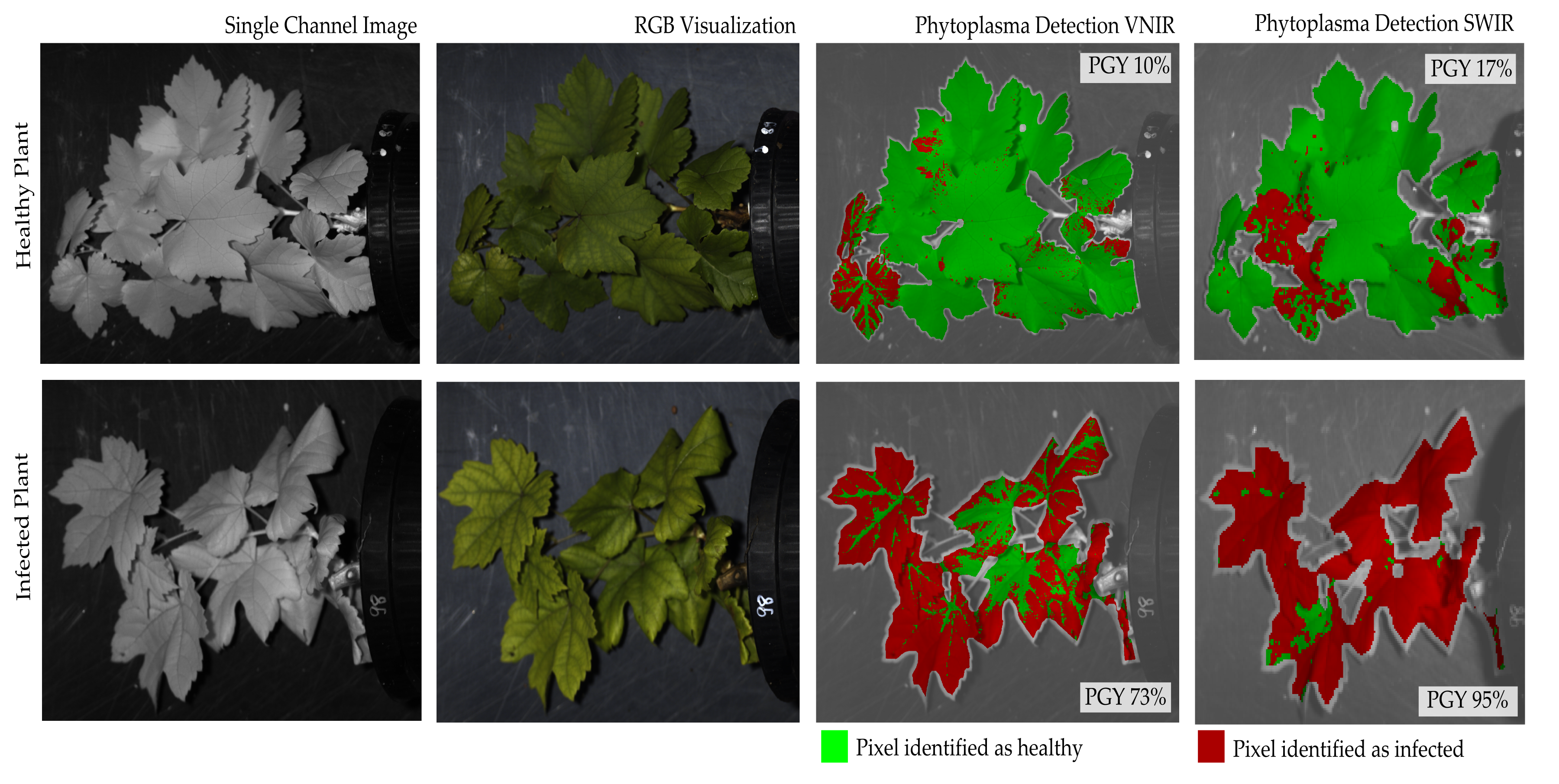
2.3. Hyperspectral Sensors and Data Acquisition

In this study, hyperspectral imaging was performed covering the spectral range from 400 to 2500 nm. For this purpose, two hyperspectral line scanning sensors (Norsk Elektro Optikk A/S, Skedsmokorset, Norway) were implemented: (i) HySpex VNIR 1800 to record spectra in the visible and near-infrared range (VNIR; 400–1000 nm) and (ii) HySpex SWIR 384 that captures the short-wave infrared range (SWIR; 1000–2500 nm). Further sensor details can be found in

Table 3. Overview of the camera specifications.

Specification	HySpex VNIR 1800	HySpex SWIR 384
Wavelength range (nm)	400–1000	1000–2500
Spectral bands	256	288
Spectral pixels	1800	384
Spectral resolution (nm)	3.26	5.45
Spatial resolution (mm/pixel)	0.17	0.65
Field of view	17°	16°
Maximum framerate (Hz)	100	400
Dynamic range (bit)	16	16
Detector type	CMOS	MCT at 150 K

.

In Figure 1, the experimental setup for hyperspectral data acquisition is depicted. In order to achieve reproducible measuring conditions, hyperspectral data were captured in an imaging Blackbox with which disturbing environmental factors can be avoided. Plant samples were placed as flat as possible in the Blackbox and the two sensors were moved in 1 m distance above the samples by a horizontal translation stage to obtain spatial images yielding the spatial resolution given in Table 3. For illumination, a 1000 W short-wave halogen spotlight (Hedler C12, Hedler Systemlicht, Runkel/Lahn, Germany) was installed between the cameras. A low reflective support surface assured minimal reflectance in the image background. In every image, a PTFE (polytetrafluoroethylene) spectralon (Sphere Optics GmbH, Herrsching, Germany) was included for calibration. The cameras’ integration time was set to yield ~90% signal within the cameras’ dynamic range. Camera frame period was set by the image acquisition software to match the driving speed of the linear stage in order to get a geometrically correct image. Image acquisition and radiometric calibration was performed using the camera vendor’s acquisition software HySpex Ground.

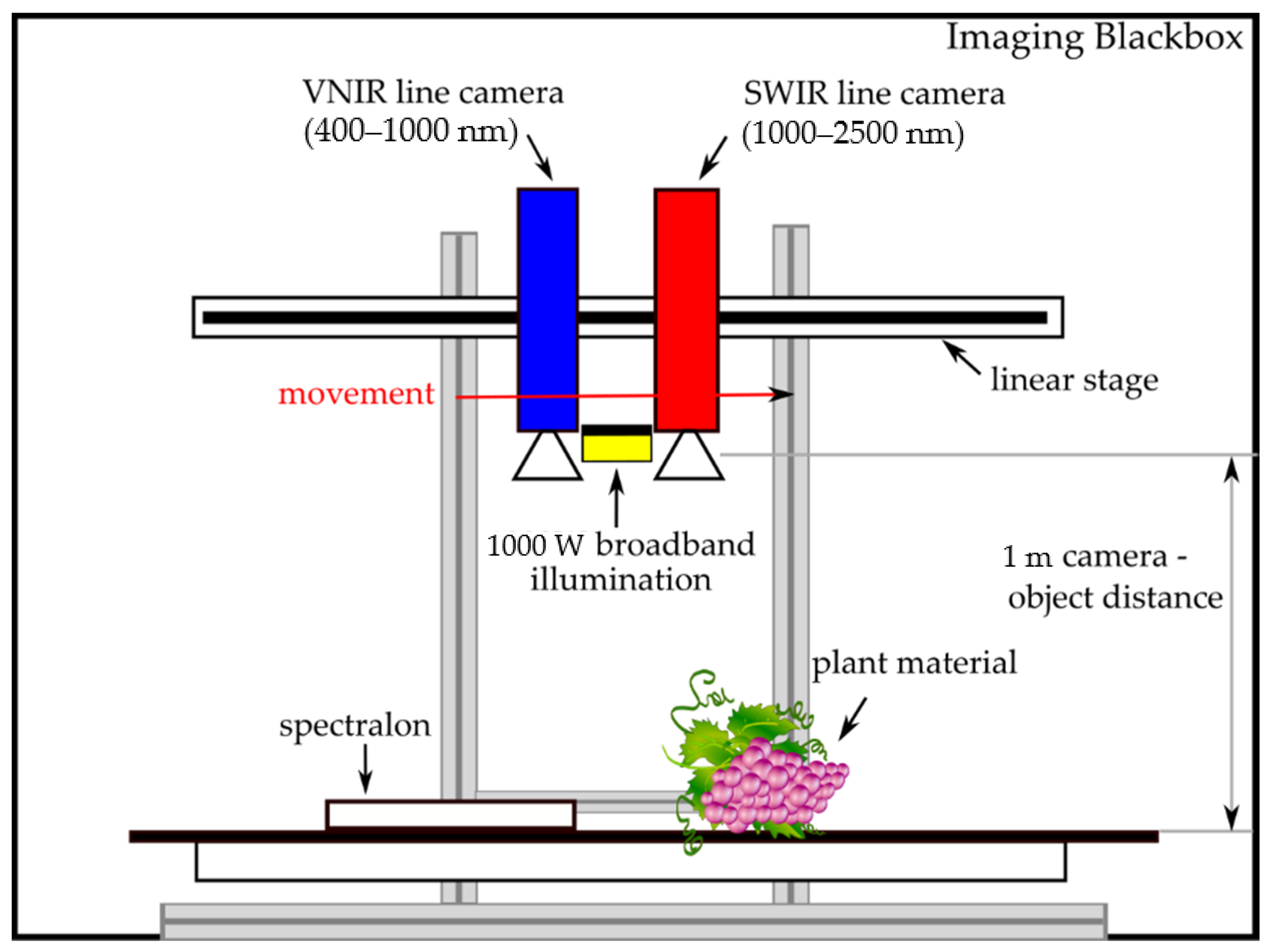
2.4. Data Calibration and Labeling

Data calibration and labeling was performed similar to previous studies [32,33]. Calibration measurements were performed before and after every plant sample. For this purpose, reflectance $R_{\lambda }$ per pixel was calculated as

$$R_{\lambda }=\frac{I_{\lambda }-I_{\lambda }^{DC}}{I_{\lambda }^W-I_{\lambda }^{DC}},$$

(1)

where $I_{\lambda }$ is the image pixel intensity at wavelength $\lambda$, $I_{\lambda }^W$ the intensity while recording the spectralon device (white reference), and $I_{\lambda }^{DC}$ the intensity when measured with closed camera shutter (dark current). Values for white and dark values were obtained individually per pixel on the scan line in order to compensate for illumination gradients generated by the halogen light source.

In order to remove background and nonrelevant sample parts like stems and pots, a segmentation for the leaf material was performed. For this purpose, a number of images was labeled by hand and a model based on the reflectance spectrum was trained to classify each spectral pixel into vegetation, background, and nonrelevant sample parts. Multi-Layer Perceptron (MLP) [34] with SNV normalization [35] performed the best and was, therefore, used for all segmentation purposes. The model training was performed using the AutoML platform HawkSpex^®Flow developed by the Fraunhofer IFF. Data from both cameras were treated separately throughout the study resulting in different models for VNIR and SWIR images. An image registration was attempted but did not yield satisfactory results. For this matter, we used MATLAB’s (MathWorks Inc., Natick, MA, USA) methods for phase correlation and nonrigid image registration. Registration was performed using two grey value channel images from both cameras (VNIR at 785 nm and SWIR at 1056 nm). The VNIR camera was mapped to the SWIR camera that has a lower resolution. The same image registration mapping was then applied to all SWIR channel images. In order to generate a labeled dataset for the subsequent modeling, data were labeled using the provided laboratory results (Table 1 and Table 2). Based on the visual assessment and the molecular analysis, all pixels per plant were labeled as either healthy or infected. For each label class, 10,000 pixel-spectra were randomly sampled from all available imaging data. This was seen as good compromise between data representation and computational demand for generating the subsequent models. Figure 2 summarizes the steps from image acquisition over pre-processing to data modeling.

2.5. Model Development and Application

Each detection problem in this paper can be described as a binary classification problem with two classes: infected vs. healthy. In order to map the spectral reflectance data to a detection decision, a machine learning approach was followed yielding a Soft-Sensor detection system [36]. In this study, a number of spectral pre-processing methods in combination with machine learning models were tested for their detection performance (

Table 4. Pre-processing methods used in this study. Calculation is performed on the dataset to generate the input to the machine learning process.

Method	Formula
Vector L2 normalization	$R_{\lambda }^N=\frac{R_{\lambda }}{\sqrt{{{\displaystyle \sum }}_{\lambda }{R}_{\lambda }{}^2}}$
Vector SNV normalization [34]	$R_{\lambda }^N=\frac{R_{\lambda }-\frac{1}{N}{{\displaystyle \sum }}_{\lambda }{R}_{\lambda }}{\sqrt{\frac{1}{N-1}{{\displaystyle \sum }}_{\lambda }{\left(R_{\lambda }-\frac{1}{N}{{\displaystyle \sum }}_{\lambda }{R}_{\lambda }\right)}^2}}$

and

Table 5. Model hyper-parameters used in this study.

Method	Hyper-Parameter	Reference
Linear Discriminance Model (LDA)	No hyperparameters	[37]
Partially Least Square (PLS)	Number of components: 20	[38]
Multi-Layer Perceptron (MLP)	Number of hidden layers: 3 Optimization method: scaled conjugate gradient backpropagation Neurons per hidden layer: 50, 25, 10	[34,39]
Radial-Basis Function Network with Relevance (rRBF)	Number of radial basis functions: 30 Optimization method: scaled nonlinear conjugate gradient	[40,41,42]

). Pre-processing is typically performed on reflectance data to minimize the effect of geometry on the measured reflectance, which leads to offset and gain effects [34]. Output of the pre-processing is then used as input to the machine learning model. In Table 4, the pre-processing methods used in this study are listed.

Hyperspectral data of this study were analyzed using four different machine learning algorithms. These include: (i) Linear Discriminance Model (LDA), (ii) Partially Least Square (PLS), (iii) Multi-Layer Perceptron (MLP), and (iv) Radial-Basis Function Network with Relevance (rRBF) (Table 5). The chosen methods differ in how data classes are separated. The LDA and PLS model use a single linear hyperplane as decision boundary, but acquire their parameters through different optimization methods. While LDA optimizes for class discrimination, PLS optimizes for input to output correlation. The MLP and rRBF model use non-linear models for a more complex decision boundary. The MLP generally works best for datasets, which can be separated using a small number of hyperplanes, whereas an RBF network is able to separate more complex shaped data clusters, since it uses receptive fields in combination with hyperplanes. For the output of these models, a coding of −1 for control/healthy and +1 for pathogen infection was used.

In order to test the model on unseen data, an n-fold cross validation with n = 10 was performed with the dataset being divided into n parts. The model was then optimized on n–1 folds while being tested on the n^th-fold. The modeling process was performed with all possible combinations without repetition of folds. As a model performance indicator, the average and standard deviations of the performance value was calculated across modeling runs and reported in the result tables.

Performance of all models was assessed using the following performance criteria (with sample being defined as one spectrum labeled with its respective class):

• Classification Accuracy (CA): Ratio calculated from the number of samples correctly classified among all possible samples.
• True Positive Rate (TPR): Ratio calculated from the number of samples detected correctly as infected among all possible infected samples.
• False Positive Rate (FPR): Ratio calculated from the number of samples detected incorrectly as infected among all possible control samples.

After model training, the best performing model in terms of classification accuracy was selected and applied to the hyperspectral images resulting in a label for each vegetation pixel. In order to evaluate the detection performance of the selected model, percentage of all considered vegetation pixels classified as either healthy or infected was calculated and the label with the highest occurrence was regarded as the representing label for the plant sample (majority vote) (Figure 3).

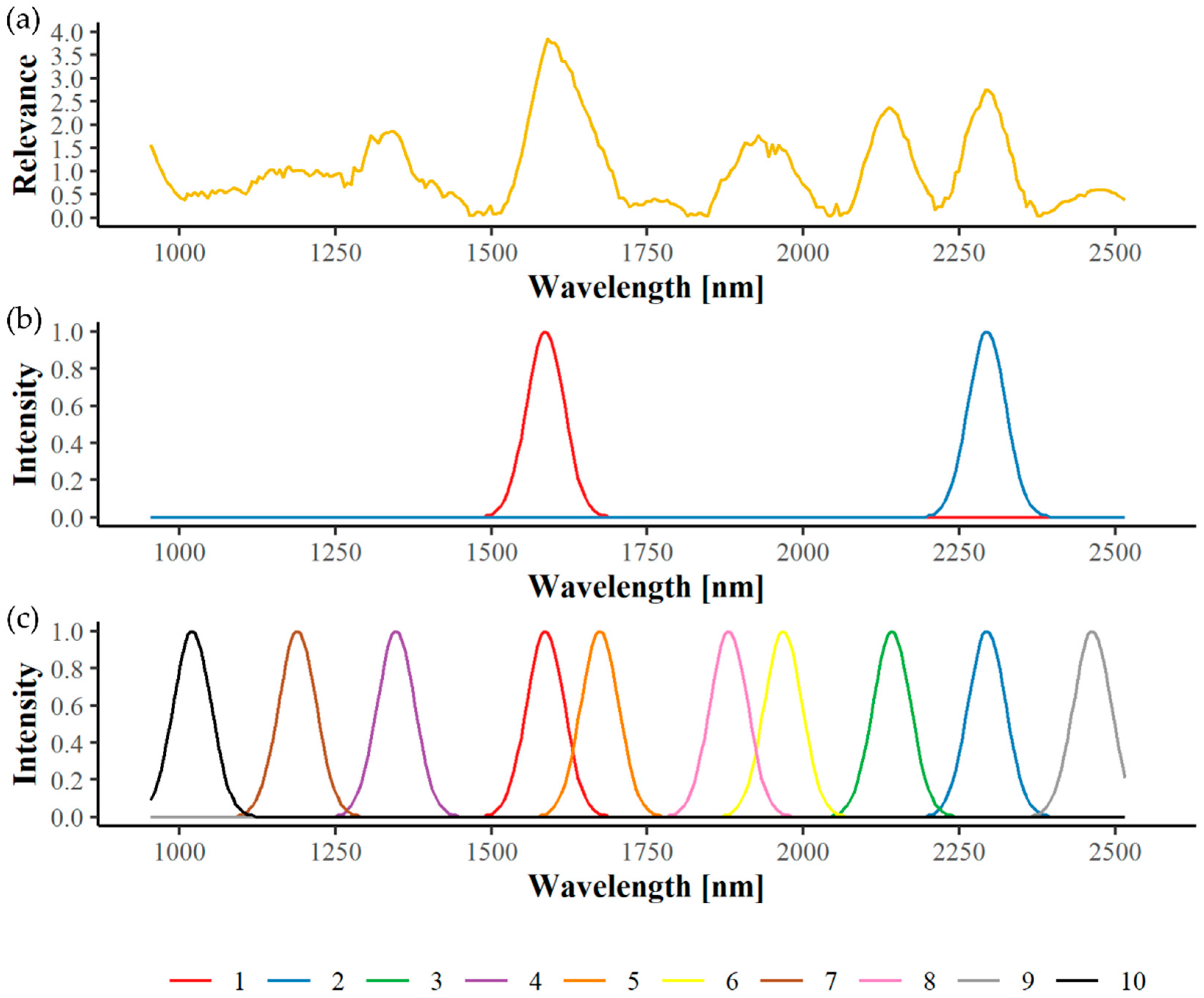
2.6. Spectral Relevance and Important Wavelengths

While optimizing the Radial Basis Function Network (RBF), a weighting per wavelength is optimized as well and indicates the importance or relevance of a wavelength’s contribution to the detection task [41]. Due to the high correlation of wavebands, such a weighting profile is rarely only activated at a single wavelength. In addition, a multispectral camera system measures reflectance with a resolution that is approximately an order of magnitude lower than that of a hyperspectral camera. Therefore, we developed an algorithm with which multispectral channels can be placed at optimal positions in the spectral range and the relevant waveband utilization can be maximized [43]. For this purpose, the relevance profile was used as probability density function (pdf), and an automatic algorithm was applied that generated 100,000 random wavelength values based on this pdf. Consequently, the generated values are denser in areas of high relevance than in areas of low relevance. This data set was then used to train a Neural Gas vector quantization algorithm [44], which placed a set number of wavelength values in a way to minimize the quantization error measured by the mean squared error between placed wavelengths and best machine generated wavelengths. Naturally, the Neural Gas algorithm covered denser areas with more wavelength candidates than less dense areas. Wavelength candidates were then ordered by their interpolated value from the relevance curve. Consequently, the first wavelength candidate is of highest importance to the detection task and relevance decreases from wavelength candidate to next wavelength candidate. Therefore, a maximum of 10 wavelength candidates for VNIR and SWIR were set in this study, as more were not considered useful. An example of the wavelength selection process is given in Figure 4.

3. Results

3.1. Model Evaluation

3.1.1. Greenhouse Plants

In this study, four different machine learning models were applied to the hyperspectral data recorded.

Table 6. Results of the different machine learning approaches for disease detection of symptomatic and nonsymptomatic greenhouse plants. Best machine learning approach according to its classification accuracy is highlighted in bold.

Disease	Symptoms	Model	Classification Accuracy (%)		True Positive Rate (%)		False Positive Rate (%)
			VNIR	SWIR	VNIR	SWIR	VNIR	SWIR
PGY	Yes	LDA	77	88	78	85	24	9
		PLS	77	88	77	86	24	9
		MLP	86	88	83	85	22	10
		rRBF	89	92	89	90	11	5
BN	Yes	LDA	62	65	57	64	26	29
		PLS	63	65	54	64	28	34
		MLP	68	73	65	72	30	27
		rRBF	70	74	68	79	30	15
BN	No	LDA	58	60	52	64	36	44
		PLS	59	60	57	62	39	42
		MLP	62	62	63	65	37	46
		rRBF	63	64	68	79	33	36

BN: Bois noir; PGY: Palatinate grapevine yellows; LDA: Linear Discriminance Model; PLS: Partially Least Square; MLP: Multi-Layer Perceptron Network; rRBF: Radial-Basis Function Network; VNIR: visual and near infrared; SWIR: short-wave infrared.

shows CAs, TPRs, and FPRs of all models for the detection of phytoplasma-infected greenhouse plants. Clear differences could be seen between the performances of the four models within each detection task. While LDA and PLS with comparable results performed the worst, MLP achieved significantly higher CAs and TPRs. However, rRBF performed best, thus, was further used to analyze greenhouse plants.

3.1.2. Field Samples

The same four models were also used to analyze symptomatic and nonsymptomatic shoots collected in the field. Results of the different machine learning approaches are given in

Table 7. Results of the different machine learning approaches for disease detection of symptomatic field material derived from red- and white-berried cultivars. Best machine learning approach according to its classification accuracy is highlighted in bold.

Disease	Symptom Coloration	Model	Classification Accuracy (%)		True Positive Rate (%)		False Positive Rate (%)
			VNIR	SWIR	VNIR	SWIR	VNIR	SWIR
PGY	White	LDA	96	75	95	75	4	26
		PLS	96	99	95	97	4	0
		MLP	97	99	97	98	3	1
		rRBF	96	98	96	97	3	1
BN	White	LDA	88	89	84	82	8	3
		PLS	88	90	84	82	8	3
		MLP	89	90	86	85	7	5
		rRBF	88	91	84	86	8	3
BN	Red	LDA	92	94	86	91	1	3
		PLS	92	95	86	91	1	2
		MLP	94	94	90	93	3	4
		rRBF	93	96	89	94	2	2

BN: Bois noir; PGY: Palatinate grapevine yellows; LDA: Linear Discriminance Model; PLS: Partially Least Square; MLP: Multi-Layer Perceptron Network; rRBF: Radial-Basis Function Network; VNIR: visual and near infrared; SWIR: short-wave infrared.

. In contrast to greenhouse plants, no significant differences could be observed between the models as their performances were almost similar within each detection task. However, MLP performed slightly better and was, therefore, further used to analyze samples collected in the field.

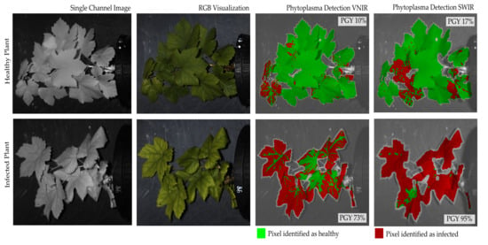
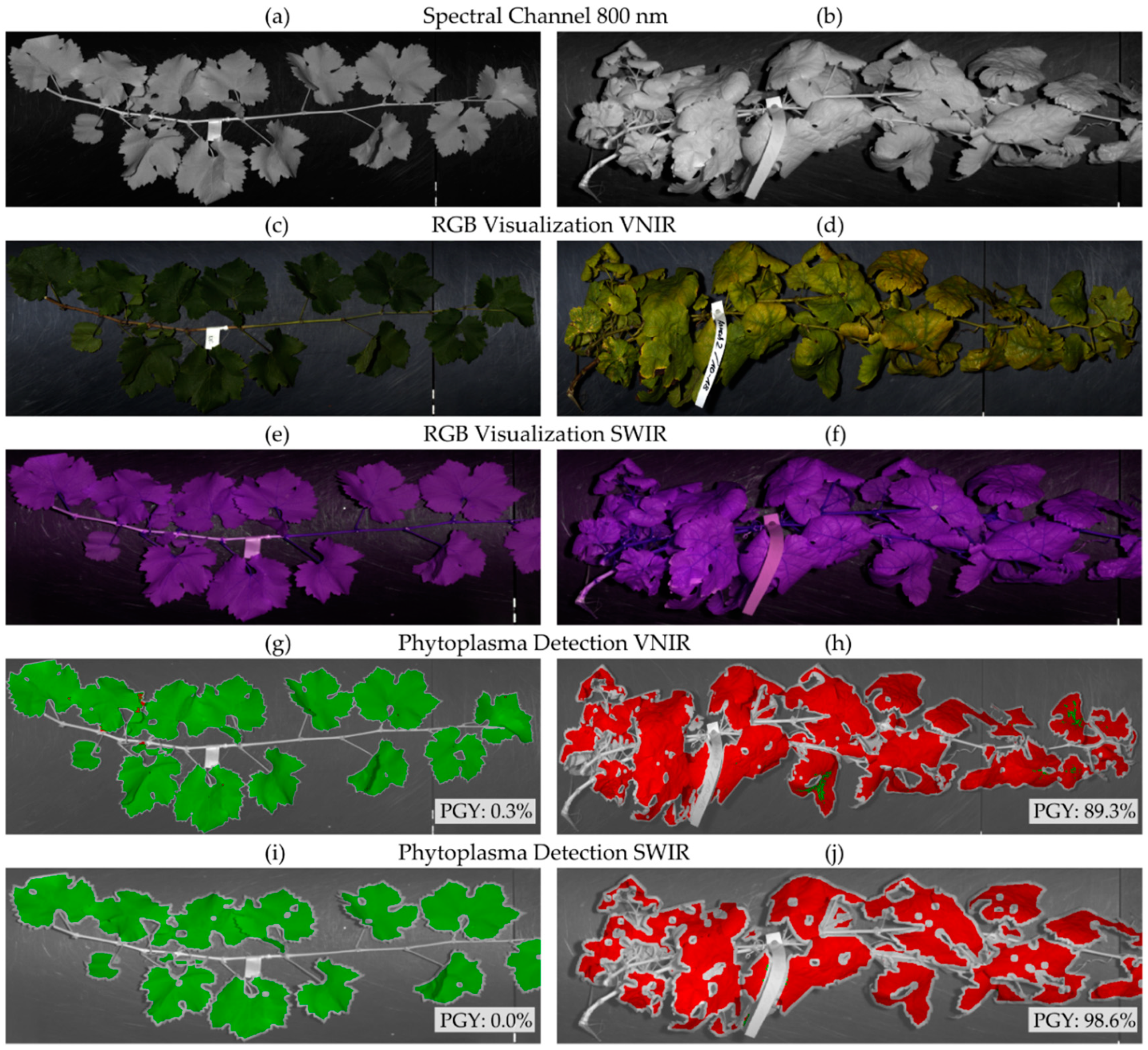
3.2. Model Application

3.2.1. Symptomatic Greenhouse Plants

During model development, all pixels were evaluated without considering spatial scales. In order to achieve a decision per vine, these models were then applied on plant scale. A majority voting of all pixel results was performed, whereby the whole plant was classified as either healthy or infected.

Table 8. Results for the detection of phytoplasma-infected and symptomatic greenhouse plants using Radial-Basis Function Network.

			VNIR	SWIR
Application per Plant		CA (%)	84	96
	PGY	TPR (%)	100	100
		FPR (%)	17	4
		CA (%)	68	79
	BN	TPR (%)	81	81
		FPR (%)	34	22

BN: Bois noir; PGY: Palatinate grapevine yellows; CA: classification accuracy; TPR: true-positive rate; FPR: false-positive rate; VNIR: visual and near infrared; SWIR: short-wave infrared.

shows the results for the detection of phytoplasma-induced leaf symptoms of greenhouse plants. Identification of PGY-induced symptoms appeared to be easier than the detection of BN-induced symptoms, which is indicated by higher TPRs and corresponding lower FPRs. Here, TPRs of 81% and 100% could be achieved for BN and PGY, respectively, in both wavelength ranges. However, FPRs were significantly higher in the VNIR range, making the SWIR range the better predictor of plants’ disease status.

3.2.2. Nonsymptomatic Greenhouse Plants

The detection of infected but symptomless plants was only possible for BN.

Table 9. Results for the detection of Bois noir-infected but symptomless greenhouse plants using Radial-Basis Function Network.

		VNIR	SWIR
Application per Plant	CA (%)	68	64
	TPR (%)	63	86
	FPR (%)	29	41

CA: classification accuracy; TPR: true-positive rate; FPR: false-positive rate; VNIR: visual and near infrared; SWIR: short-wave infrared.

shows CAs, TPRs, and FPRs for the model application on plant level. Identification of symptomless greenhouse plants seemed to be more challenging than the detection of symptomatic plants as is indicated by lower model performance. TPRs of 68% and 79% were achieved for VNIR and SWIR, respectively. However, 29% (VNIR) and 41% (SWIR) of all pixels were falsely classified as symptomatic leading to rather low CAs of 68% and 64% for VNIR and SWIR, respectively.

3.2.3. Symptomatic Field Material

Symptom detection seemed to be easier for shoots collected in the field than for greenhouse plants (

Table 10. Results for the detection of symptomatic phytoplasma-infected shoots taken from the field using Multi-Layer Perceptron.

	Disease	Symptom Coloration		VNIR	SWIR
Application per Plant			CA (%)	100	100
	PGY	White	TPR (%)	100	100
			FPR (%)	0	0
			CA (%)	96	96
	BN	White	TPR (%)	96	95
			FPR (%)	7	0
			CA (%)	98	98
	BN	Red	TPR (%)	97	97
			FPR (%)	0	0

BN: Bois noir; PGY: Palatinate grapevine yellows; CA: classification accuracy; TPR: true-positive rate; FPR: false-positive rate; VNIR: visual and near infrared; SWIR: short-wave infrared.

). Satisfying results could be accomplished for both diseases with TPRs of 95–100% and FPRs of 0–7%. Although symptom detection was successful for both diseases, PGY performed slightly better reaching detection rates of 100% without misclassifications. In general, no differences could be seen between VNIR and SWIR, so, both wavelength ranges seem to be suitable for the differentiation task.

3.3. Spectral Relevance and Important Wavelengths

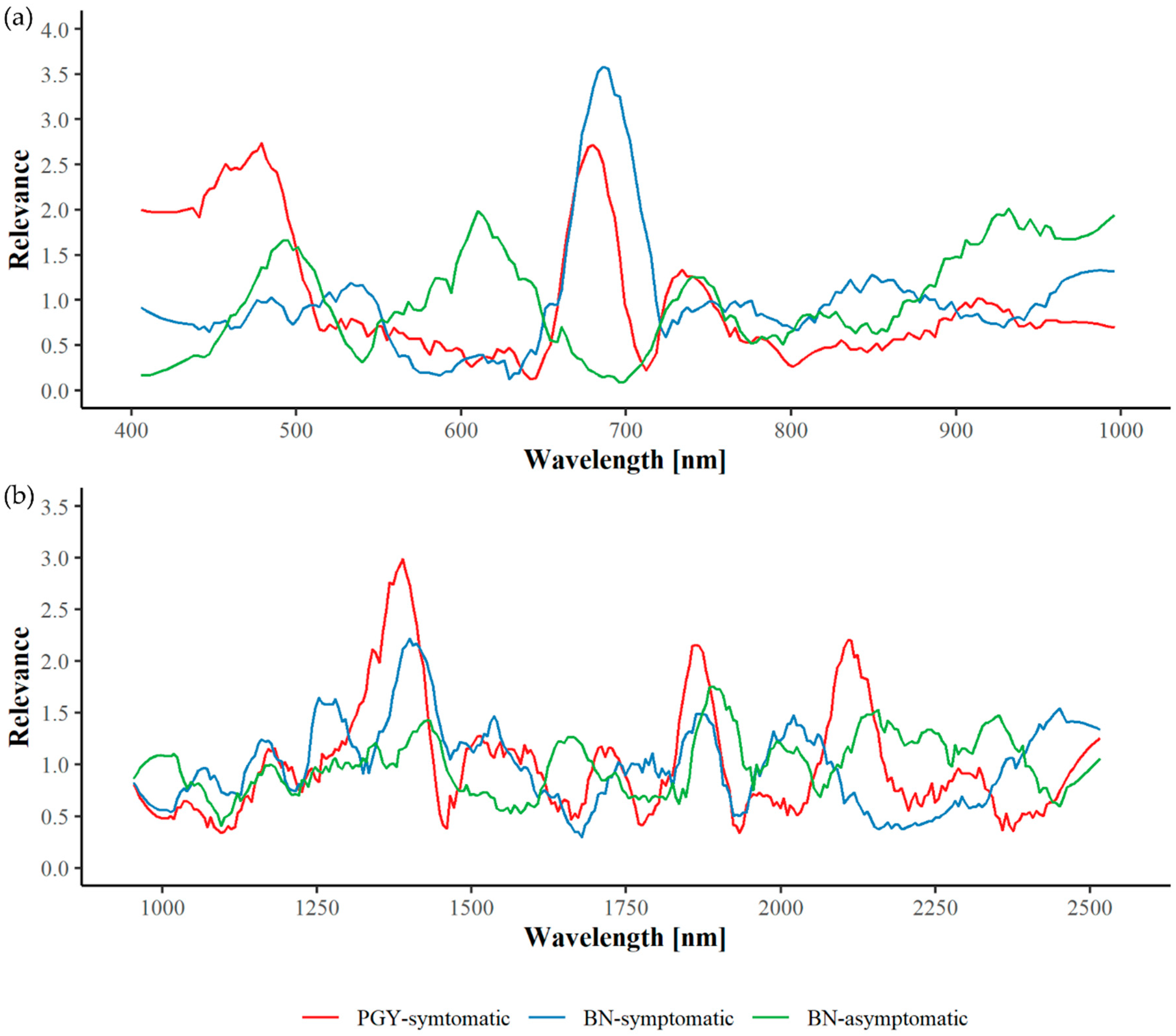
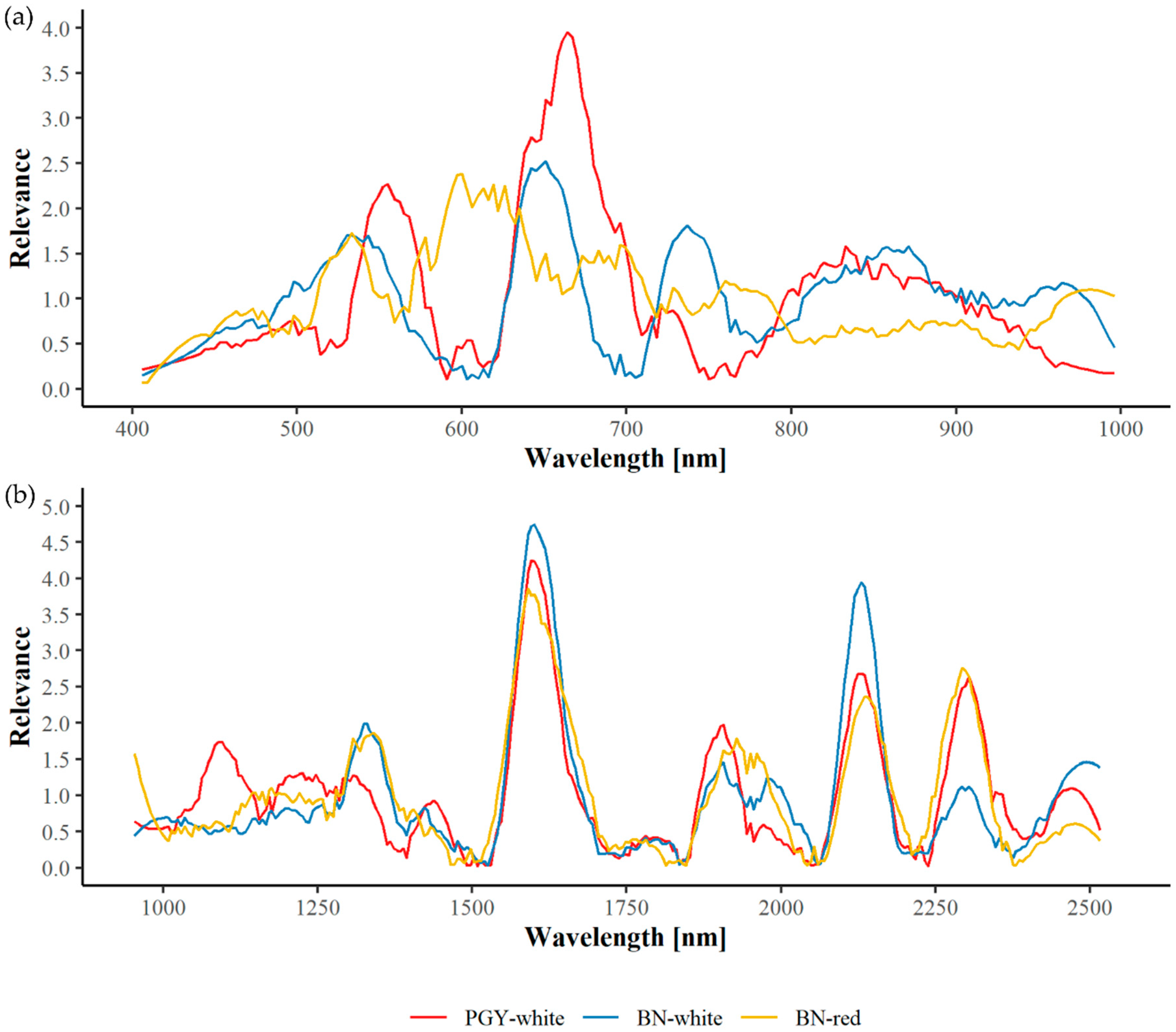
3.3.1. Greenhouse Plants

The machine learning approach allows the calculation of relevance profiles that provide information about the most important wavelengths for the detection tasks. Relevance profiles for the identification of phytoplasma-infected greenhouse plants are depicted in Figure 5. Based on these relevance profiles up to 10 local maxima were selected. They are listed according to their importance in

Table 11. The 10 most informative spectral bands for the detection of phytoplasma-infected greenhouse plants.

Disease	Symptoms	VNIR										SWIR
		1	2	3	4	5	6	7	8	9	10	1	2	3	4	5	6	7	8	9	10
PGY	Yes	679	459	492	423	748	905	965	541	832	606	1373	1861	2125	1545	1709	2288	1214	2459	2000	1031
BN	Yes	689	971	861	539	486	752	914	811	431	631	1400	2451	1865	2010	1549	1239	1160	1734	1055	2313
BN	No	932	975	503	616	890	734	579	835	455	784	1893	1433	2180	2362	1658	1343	2000	2268	2102	1170

BN: Bois noir; PGY: Palatinate grapevine yellows; 1–10: selected spectral bands; VNIR: visual and near infrared; SWIR: short-wave infrared.

. Clear differences can be seen in the three differentiation tasks in both VNIR and SWIR.

Regarding symptomatic plants infected with PGY, most important wavelengths in VNIR are around 459–492 and 679 nm with some minor peaks at 748 and 905 nm. The peak around 679 nm overlaps with that of BN-infected and symptomatic plants at 689 nm showing the importance of this spectral region for the discrimination of symptomatic and control plants. However, no further concordance could be shown between the two diseases. Regarding BN-infected but symptomless plants, wavelengths at 503, 616, and 734 nm as well as in the range of 932–972 nm seem to be of highest relevance.

In the SWIR range, wavelengths around 1400 and 1865 nm are of importance for all three detection tasks, although peaks seem to be slightly shifted. Further significant wavelengths for the identification of PGY-symptomatic plants are 1545, 1709, and 2125 nm. Regarding BN-infected plants, wavelengths around 1239, 1549, 2010, and 2451 nm are highly relevant for the detection of symptomatic plants and wavelengths of 1343, 1658, 2000, 2180, and 2362 for asymptomatic plants.

3.3.2. Field Material

Relevance profiles for the detection of symptomatic field material are depicted in Figure 6 and exact wavelengths are given in

Table 12. The 10 most informative spectral bands for the detection of symptomatic phytoplasma-infected shoots taken from the field.

Disease	Cultivar	VNIR										SWIR
		1	2	3	4	5	6	7	8	9	10	1	2	3	4	5	6	7	8	9	10
PGY	White	672	639	557	845	891	801	498	718	945	443	1587	2132	2305	1648	1918	1072	1239	2458	1784	1391
BN	White	637	741	667	862	553	966	509	812	913	452	1582	2131	1649	1353	2466	1981	2297	1204	1869	1034
BN	Red	626	528	586	673	773	969	718	458	899	839	1586	2294	2140	1347	1670	1965	1188	1881	2462	1019

BN: Bois noir; PGY: Palatinate grapevine yellows; 1–10: selected spectral bands; VNIR: visual and near infrared; SWIR: short-wave infrared.

. Regarding PGY, most important wavelengths are around 557, 639, 672, and in the range of 801–940 nm. Some of these are also relevant for the identification of BN-infected shoots of white varieties, e.g., 637, 553, and 812–966 nm with an additional important wavelength at 741 nm. Obvious differences become visible between symptomatic shoots of white and red varieties with 528, 586–626, and 673 nm being the key wavelength ranges for the detection of BN-symptomatic shoots in red varieties.

In contrast, a clear pattern can be seen in SWIR with wavelengths around 1585, 2135, and 2300 nm being of relevance in all three differentiation tasks. Small differences between PGY and BN-infected shoots can be found between 1880 and 2000 nm. Here, important wavelengths are slightly shifted. Further differences become apparent in the range of 1050–1490 nm, with 1072 nm being important for the identification of PGY and 1350 nm for BN.

However, when comparing relevance spectra of greenhouse plants and field material only a few concordances can be found, for PGY, at 675 and 2130 nm and for BN, only at around 540 nm.

4. Discussion

For high dimensional data, it is difficult to determine the best machine learning model in advance as every model underlies different mathematical conditions, which may lead to different performances when applied on the same dataset. Therefore, four different machine learning models were tested in this study. While for greenhouse plants rRBF showed highest CAs and TPRs, MLP performed best for shoots collected in the field. High-dimensional data are not easy to visualize in order to check if the datasets meet one of the mentioned conditions. The training was done using careful validation and performed on identical dataset splits in order to generate comparable results. Furthermore, we analyzed the relevance of wavelengths ranges for more interpretability of the modeling outcome. Comparing different classification algorithms is a common approach in hyperspectral data analysis as has been shown in various studies. For the detection of Botrytis cinerea and Colletotrichum acutatum infections on strawberry fruits, Siedliska et al. [45] analyzed four different classification methods of which a Backpropagation Neural Network (BNN) showed highest accuracy. Wiegmann et al. [46] used PLS, MLP, and an RBF network with Transfer Learning for the prediction of nutrient content in barley grain. Here, PLS was identified as the best compromise between good prediction performance and lowest computing demand. For the detection of laurel wilt disease on avocado plants, Abdulridha et al. [47] also applied MLP as well as RBF neural networks and additionally performed a stepwise discriminant (STEPDISC) analysis on hyperspectral data in the VNIR region. In both early and late infection stages, MLP performed significantly better than STEPDISC and RBF.

Symptom development of BN and PGY is known to be influenced by environmental factors, scion-rootstock combination, and the grapevine cultivar [1]. Therefore, ungrafted vines grown under controlled greenhouse conditions were used as a first approach to assess the potential of hyperspectral imaging for GY disease detection. While high classification rates could be achieved for PGY-infected plants, BN symptom detection performed significantly worse with CAs of 68% and 79% for VNIR and SWIR, respectively. Although symptoms of GY are indistinguishable, their appearance on a vine may differ. Phytoplasmas associated to the 16SrV group like PGY or FD usually induce systemic symptoms, thus, affecting the entire plant. BN-infected vines, however, express symptoms only partially on some shoots, while others seem to remain healthy [2]. This could also be observed for greenhouse plants in the present study. PGY-infected plants showed symptoms along the whole shoot; in contrast, vines infected by BN developed only some symptomatic leaves and symptoms did not further expand as the season progressed. This mixture of symptomatic and nonsymptomatic leaves might be the reason for lower CAs in BN-infected greenhouse plants, especially since disease detection was performed successfully using plant material collected in the field.

In general, phytoplasmas are erratically distributed in their host plants and their location as well as titer are assumed to play a significant role in symptom development [48]. In combination with the fact that some cultivars, most rootstocks, and wild Vitis species may be completely symptomless [12], identifying disease carriers would be a key element in reducing pathogen reservoirs in vineyards and nurseries and especially in rootstock motherblocks. The feasibility of such an approach has already been demonstrated for other phloem-limited pathogens such as citrus tristeza virus or grapevine leafroll-associated viruses [32,49]. Unfortunately, the detection of BN-infected but symptomless plants was not successful under greenhouse conditions, since VNIR and SWIR showed poor classification performances of 68% and 64%, respectively, which is close to a random classifier. Since results for symptom detection were significantly higher for PGY- than BN-infected vines, it would be interesting to evaluate in further studies whether this effect could also be observed in symptomless PGY-infected plants.

Even though analyzing greenhouse-grown vines allows environmental factors to be precisely controlled, phenotypes strongly differ from those grown in the field since grapevines are naturally large perennial plants. Therefore, as a next step, shoots collected in the field were recorded under laboratory conditions. In general, better results could be obtained for plant material from the field than for greenhouse plants. This might be due to a higher amount of symptomatic leaves per sample as shoots from field-grown grapevines were completely symptomatic and considerably larger than greenhouse vines. Moreover, symptoms slightly varied between greenhouse and field. As the season progresses, symptomatic leaves may turn crispy and brittle [11], thereby, influencing especially the NIR spectral range that is strongly affected by cell tissue structures [15]. However, this could only be observed for field material and not for greenhouse plants. Furthermore, Mannini et al. [50] found that vegetative propagation of infected vines might lead to reduced infection intensity in the progeny, which could also be one reason for lower CAs in greenhouse plants.

In summary, disease detection could be performed successfully for both BN and PGY using field-grown plant material leading to the assumption that these two GY may also be detectable directly in the field, as has been demonstrated for FD [23,24,25,26,27]. Identifying the most relevant wavelengths for a multispectral disease detection system and, as a result thereof, reduced data dimensionality might be a promising concept for transferring BN and PGY detection into the field. Assessment of optimal spectral bands is a common approach that has widely been used for the detection of tomato spotted wilt virus [51], anthracnose on strawberries [52], three sugar beet diseases [53], or powdery mildew and Esca on grapevines [33,54]. In this study, a maximum of 10 relevant wavelength bands were selected separately for VNIR and SWIR, as more were not considered realistic for multispectral systems. Many of these wavelengths could be found in the visible range of the electromagnetic spectrum for both greenhouse plants and field material. Phytoplasmas are known to inhabit the phloem of their host plants, thus, callose is deposited near sieve plates and plasmodesmata to hinder pathogen spread [55]. As a consequence thereof, phloem transport is inhibited leading to an impairment of photosynthetic activity [56]. Moreover, infection typically causes a decrease in chlorophylls and carotenoids [57]. These changes in pigment content are predominantly expressed in the range of 400–700 nm [58]. Chlorophyll a and b strongly absorb incoming light in the blue and red region of the spectrum, thereby providing energy for photosynthesis [59]. Besides chlorophylls, carotenoids are the main factors influencing reflectance characteristic in the visible range of light, especially in the blue region [60]. The differences observed in VNIR reflectance spectra of BN-infected field material collected from red- and white-berried grapevines may be explained by an increase in anthocyanin content during symptom development [61] that is not observable in white cultivars since they lack several genes of the flavonoid biosynthetic pathway [62]. Anthocyanins affect leaves’ reflectance mainly around 550 nm. Based on this finding, Gitelson et al. [63] introduced the anthocyanin reflectance index (ARI). In general, several vegetation indices (VIs) have been described to estimate leaves’ pigment contents [16,64] and some of them might be applicable to the spectral data of this study. However, common VIs typically lack disease specificity, therefore, attempts have been made to develop individual spectral disease indices (SDIs) [53]. The generation of optimal wavelength pairs for suitable BN and PGY indices might be a subject for further studies.

Regarding relevance profiles in the SWIR range, a consistent pattern could be seen for field material across the three detection tasks with 1585, 2135, and 2300 nm being of high importance. As described by Curran et al. [59], wavelengths around 1580 nm are strongly associated to the absorption of starch and sugar. Due to the disturbed photosynthesis and phloem blockage upon phytoplasma infection, synthesis and transport of carbohydrates and starch are modified leading to their accumulation in mature leaves [65]. Furthermore, phytoplasma infection may cause a significant decrease in lignin content [66]. According to Nagler et al. [67], cellulose and lignin have a relatively broad absorption feature around 2100 nm. In general, the range of 2100–2300 nm is not only heavily affected by leaf cellulose and lignin but also by protein content [68] that is known to be strongly reduced in many phytoplasma-infected plants [69]. However, these changes typically occur in heavily affected leaves only, which could explain the differences between relevance profiles of greenhouse and field material as field material was more affected by phytoplasma infection.

The results of this study are based on 1-year data; therefore, selected spectral bands need to be verified in further experimental years. Sinha et al. [70] identified relevant wavelengths for the identification of grapevine leafroll-associated virus 3 in Cabernet Sauvignon vines over two consecutive years, but transfer of these wavelengths from one year to the other was only partially satisfying. Moreover, Al-Saddik et al. [27,71] tried to assess optimal spectral bands for FD detection in different white and red grapevine cultivars, but the best bands selected were different from one case to another. Nevertheless, in further studies, it will be of interest to transfer BN and PGY detection to the field.

5. Conclusions and Perspectives

In this study, greenhouse plants and shoots collected in the field were analyzed under controlled laboratory conditions to evaluate the potential of hyperspectral imaging for disease detection. So far, no similar work on BN and PGY has been conducted as previous studies focused mainly on FD. While identification of PGY-infected greenhouse plants was successful reaching CAs of up to 96%, symptom detection of BN needs to be improved. Further investigations will also be necessary for infected but symptomless plants. Identification of these plants could help to improve nurseries’ ability to provide phytoplasma-free propagation material. However, symptomatic field material could be easily classified with CAs of 96–100%. Further studies could expand upon our work by transferring the developed disease detection models into the field. For viticulture, a tractor-mounted system might be a suitable method since data could be collected in parallel to fieldwork. An airborne approach using UAVs could be a fast and flexible alternative. For this purpose, it would be useful to develop a multispectral sensor using phytoplasma-specific wavelength bands, thereby, reducing data dimensionality and computational time. As a first step, the most relevant wavelengths for each differentiation tasks could be identified in this study. Selected bands differed from one case to the other, except for field material in the SWIR spectral range where consistent wavelengths could be observed. So far, Germany is considered FD-free but it cannot be excluded that the disease will be present in future. Due to the relatedness of FD and PGY, results of this study could be used as a basis to develop a sensor-based monitoring system that could then help to fulfill the required quarantine restrictions. In general, many future applications are possible; therefore, complementary studies with increased number of samples should be conducted in order to validate the results presented in this work.

References

1. Angelini, E.; Constable, F.; Duduk, B.; Fiore, N.; Quaglino, F.; Bertaccini, A. Grapevine phytoplasmas. In Phytoplasmas: Plant Pathogenic Bacteria-I; Rao, G., Bertaccini, A., Fiore, N., Liefting, L., Eds.; Springer: Singapore, 2018; pp. 123–151. [Google Scholar]
2. Maixner, M.; Rüdel, M.; Daire, X.; Boudon-Padieu, E. Diversity of grapevine yellows in Germany. Vitis 1995, 34, 235–236. [Google Scholar]
3. Quaglino, F.; Zhao, Y.; Casati, P.; Bulgari, D.; Bianco, P.A.; Wei, W.; Davis, R.E. ‘Candidatus Phytoplasma solani’, a novel taxon associated with stolbur- and bois noir-related diseases of plants. Int. J. Syst. Evol. Microbiol. 2013, 63, 2879–2894. [Google Scholar] [CrossRef] [PubMed] [Green Version]
4. Sforza, R.; Clair, D.; Daire, X.; Larrue, J.; Boudon-Padieu, E. The role of Hyalesthes obsoletus (Hemiptera: Cixiidae) in the occurrence of bois noir of grapevines in France. J. Phytopathol. 1998, 146, 549–556. [Google Scholar] [CrossRef]
5. Arnaud, G.; Malembic-Maher, S.; Salar, P.; Bonnet, P.; Maixner, M.; Marcone, C.; Boudon-Padieu, E.; Foissac, X. Multilocus sequence typing confirms the close genetic interrelatedness of three distinct Flavescence dorée phytoplasma strain clusters and group 16SrV phytoplasmas infecting grapevine and alder in Europe. Appl. Environ. Microbiol. 2007, 73, 4001–4010. [Google Scholar] [CrossRef] [PubMed] [Green Version]
6. Maixner, M.; Reinert, W.; Darimont, H. Transmission of grapevine yellows by Oncopsis alni (Schrank)(Auchenorrhyncha: Macropsinae). Vitis 2000, 39, 83–84. [Google Scholar]
7. Maixner, M.; Albert, A.; Johannesen, J. Survival relative to new and ancestral host plants, phytoplasma infection, and genetic constitution in host races of a polyphagous insect disease vector. Ecol. Evol. 2014, 4, 3082–3092. [Google Scholar] [CrossRef]
8. Maixner, M.; Reinert, W. Oncopsis alni (Schrank)(Auchenorrhyncha: Cicadellidae) as a vector of the alder yellows phytoplasma of Alnus glutinosa (L.) Gaertn. Eur. J. Plant Pathol. 1999, 105, 87–94. [Google Scholar] [CrossRef]
9. Caglayan, K.; Gazel, M.; Škorić, D. Transmission of phytoplasmas by agronomic practices. In Phytoplasmas: Plant Pathogenic Bacteria-II; Bertaccini, A., Weintraub, P., Rao, G., Mori, N., Eds.; Springer: Singapore, 2019; pp. 149–163. [Google Scholar]
10. Bertaccini, A.; Duduk, B.; Paltrinieri, S.; Contaldo, N. Phytoplasmas and phytoplasma diseases: A severe threat to agriculture. Am. J. Plant Sci. 2014, 5, 1763–1788. [Google Scholar] [CrossRef] [Green Version]
11. Belli, G.; Bianco, P.; Conti, M. Grapevine yellows in Italy: Past, present and future. J. Plant Pathol. 2010, 92, 303–326. [Google Scholar] [CrossRef]
12. Eveillard, S.; Jollard, C.; Labroussaa, F.; Khalil, D.; Perrin, M.; Desqué, D.; Salar, P.; Razan, F.; Hévin, C.; Bordenave, L.; et al. Contrasting susceptibilities to Flavescence dorée in Vitis vinifera, rootstocks and wild Vitis species. Front. Plant Sci. 2016, 7, 1762. [Google Scholar] [CrossRef] [Green Version]
13. Maixner, M. Grapevine yellows—Current developments and unsolved questions. In Proceedings of the 15th Meeting of ICVG, Stellenbosch, South Africa, 3–7 April 2006; pp. 86–88. [Google Scholar]
14. Bianco, P.A.; Romanazzi, G.; Mori, N.; Myrie, W.; Bertaccini, A. Integrated management of phytoplasma diseases. In Phytoplasmas: Plant Pathogenic Bacteria-II; Bertaccini, A., Weintraub, P., Rao, G., Mori, N., Eds.; Springer: Singapore, 2019; pp. 237–258. [Google Scholar]
15. Mahlein, A.K. Plant disease detection by imaging sensors—Parallels and specific demands for precision agriculture and plant phenotyping. Plant Dis. 2016, 100, 241–251. [Google Scholar] [CrossRef] [PubMed] [Green Version]
16. Bock, C.H.; Barbedo, J.G.; del Ponte, E.M.; Bohnenkamp, D.; Mahlein, A.-K. From visual estimates to fully automated sensor-based measurements of plant disease severity: Status and challenges for improving accuracy. Phytopathol. Res. 2020, 2, 9. [Google Scholar] [CrossRef] [Green Version]
17. Arens, N.; Backhaus, A.; Doll, S.; Fischer, S.; Seiffert, U.; Mock, H.P. Non-invasive presymptomatic detection of Cercospora beticola infection and identification of early metabolic responses in sugar beet. Front. Plant Sci. 2016, 7, 1377. [Google Scholar] [CrossRef] [PubMed] [Green Version]
18. Polder, G.; van der Heijden, G.W.A.M.; van Doorn, J.; Baltissen, T.A.H.M.C. Automatic detection of tulip breaking virus (TBV) in tulip fields using machine vision. Biosyst. Eng. 2014, 117, 35–42. [Google Scholar] [CrossRef] [Green Version]
19. Behmann, J.; Bohnenkamp, D.; Paulus, S.; Mahlein, A.-K. Spatial referencing of hyperspectral images for tracing of plant disease symptoms. J. Imaging 2018, 4, 143. [Google Scholar] [CrossRef] [Green Version]
20. Delalieux, S.; Somers, B.; Verstraeten, W.W.; van Aardt, J.A.N.; Keulemans, W.; Coppin, P. Hyperspectral indices to diagnose leaf biotic stress of apple plants, considering leaf phenology. Int. J. Remote Sens. 2009, 30, 1887–1912. [Google Scholar] [CrossRef]
21. Kuska, M.; Wahabzada, M.; Leucker, M.; Dehne, H.W.; Kersting, K.; Oerke, E.C.; Steiner, U.; Mahlein, A.K. Hyperspectral phenotyping on the microscopic scale: Towards automated characterization of plant-pathogen interactions. Plant Methods 2015, 11, 28. [Google Scholar] [CrossRef] [Green Version]
22. Barthel, D.; Fischnaller, S.; Eisenstecken, D.; Kerschbamer, C.; Messner, M.; Dordevic, N.; Robatscher, P.; Janik, K. Near-infrared spectroscopy analysis—A useful tool to detect apple proliferation diseased trees? Phytopathog. Mollicutes 2019, 9, 79–80. [Google Scholar] [CrossRef]
23. Albetis, J.; Duthoit, S.; Guttler, F.; Jacquin, A.; Goulard, M.; Poilvé, H.; Féret, J.-B.; Dedieu, G. Detection of Flavescence dorée grapevine disease using unmanned aerial vehicle (UAV) multispectral imagery. Remote Sens. 2017, 9, 308. [Google Scholar] [CrossRef] [Green Version]
24. Albetis, J.; Jacquin, A.; Goulard, M.; Poilvé, H.; Rousseau, J.; Clenet, H.; Dedieu, G.; Duthoit, S. On the potentiality of UAV multispectral imagery to detect Flavescence dorée and grapevine trunk diseases. Remote Sens. 2018, 11, 23. [Google Scholar] [CrossRef] [Green Version]
25. Al-Saddik, H.; Simon, J.C.; Cointault, F. Development of spectral disease indices for ‘Flavescence dorée’ grapevine disease identification. Sensors 2017, 17, 2772. [Google Scholar] [CrossRef] [Green Version]
26. Al-Saddik, H.; Laybros, A.; Billiot, B.; Cointault, F. Using image texture and spectral reflectance analysis to detect yellowness and Esca in grapevines at leaf-level. Remote Sens. 2018, 10, 618. [Google Scholar] [CrossRef] [Green Version]
27. Al-Saddik, H.; Simon, J.-C.; Cointault, F. Assessment of the optimal spectral bands for designing a sensor for vineyard disease detection: The case of “Flavescence dorée”. Precis. Agric. 2019, 20, 398–422. [Google Scholar] [CrossRef]
28. Maixner, M.; Ahrens, U.; Seemüller, E. Detection of the German grapevine yellows (Vergilbungskrankheit) MLO in grapevine, alternative hosts and a vector by a specific PCR procedure. Eur. J. Plant Pathol. 1995, 101, 241–250. [Google Scholar] [CrossRef]
29. Lorenz, K.; Schneider, B.; Ahrens, U.; Seemüller, E. Detection of the apple proliferation and pear decline phytoplasmas by PCR amplification of ribosomal and nonribosomal DNA. Phytopathology 1995, 85, 771–776. [Google Scholar] [CrossRef]
30. Schneider, B.; Seemüller, E.; Smart, C.; Kirkpatrick, B. Phylogenetic classification of plant pathogenic mycoplasma-like organisms or phytoplasmas. In Molecular and Diagnostic Procedures in Mycoplasmology; Razin, S., Tully, J., Eds.; Academic Press: San Diego, CA, USA, 1995; Volume 1, pp. 369–380. [Google Scholar]
31. Marcone, C.; Ragozzino, A.; Seemüller, E. Detection of an elm yellows-related phytoplasma in eucalyptus trees affected by little-leaf disease in Italy. Plant Dis. 1996, 80, 669–673. [Google Scholar] [CrossRef]
32. Bendel, N.; Kicherer, A.; Backhaus, A.; Köckerling, J.; Maixner, M.; Bleser, E.; Klück, H.-C.; Seiffert, U.; Voegele, R.T.; Töpfer, R. Detection of grapevine leafroll-associated virus 1 and 3 in white and red grapevine cultivars using hyperspectral imaging. Remote Sens. 2020, 12, 1693. [Google Scholar] [CrossRef]
33. Bendel, N.; Kicherer, A.; Backhaus, A.; Klück, H.-C.; Seiffert, U.; Fischer, M.; Voegele, R.T.; Töpfer, R. Evaluating the suitability of hyper- and multispectral imaging to detect foliar symptoms of the grapevine trunk disease Esca in vineyards. Plant Methods 2020, 16, 142. [Google Scholar] [CrossRef]
34. Cybenko, G. Approximation by superpositions of a sigmoidal function. Math Control Sign. Syst. 1989, 2, 303–314. [Google Scholar] [CrossRef]
35. Asaari, M.S.M.; Mishra, P.; Mertens, S.; Dhondt, S.; Inzé, D.; Wuyts, N.; Scheunders, P. Close-range hyperspectral image analysis for the early detection of stress responses in individual plants in a high-throughput phenotyping platform. ISPRS J. Photogram. Remote Sens. 2018, 138, 121–138. [Google Scholar] [CrossRef]
36. Fortuna, L.; Graziani, S.; Rizzo, A.; Xibilia, M.G. Soft Sensors for Monitoring and Control of Industrial Processes; Springer Science & Business Media: London, UK, 2007. [Google Scholar]
37. Krzanowski, W. Principles of Multivariate Analysis: A User’s Perspective; Clarendon Press: Oxford, UK, 1988; pp. 291–301. [Google Scholar]
38. Wold, S.; Sjöström, M.; Eriksson, L. PLS-regression: A basic tool of chemometrics. Chemom. Intell. Lab Syst. 2001, 58, 109–130. [Google Scholar] [CrossRef]
39. Møller, M.F. A scaled conjugate gradient algorithm for fast supervised learning. Neural Netw. 1993, 6, 525–533. [Google Scholar] [CrossRef]
40. Moody, J.; Darken, C.J. Fast learning in networks of locally-tuned processing units. Neural Comput. 1989, 1, 281–294. [Google Scholar] [CrossRef]
41. Backhaus, A.; Bollenbeck, F.; Seiffert, U. Robust classification of the nutrition state in crop plants by hyperspectral imaging and artificial neural networks. In Proceedings of the 3rd Workshop on Hyperspectral Image and Signal Processing: Evolution in Remote Sensing (Whispers), Lisbon, Portugal, 6–9 June 2011; pp. 1–4. [Google Scholar]
42. Dehghani, R.; Mahdavi-Amiri, N. Scaled nonlinear conjugate gradient methods for nonlinear least squares problems. Numer. Algorithms 2019, 82, 1–20. [Google Scholar] [CrossRef]
43. Becker, F.; Backhaus, A.; Johrden, F.; Flitter, M. Optimal multispectral sensor configurations through machine learning for cognitive agriculture. Automatisierungstechnik Spec. Issue Cognetive Agric. 2020. Accepted for Publication. [Google Scholar]
44. Martinetz, T.M.; Berkovich, S.G.; Schulten, K.J. ‘Neural-gas’ network for vector quantization and its application to time-series prediction. IEEE Transact. Neural Netw. 1993, 4, 558–569. [Google Scholar] [CrossRef]
45. Siedliska, A.; Baranowski, P.; Zubik, M.; Mazurek, W.; Sosnowska, B. Detection of fungal infections in strawberry fruit by VNIR/SWIR hyperspectral imaging. Postharvest Biol. Technol. 2018, 139, 115–126. [Google Scholar] [CrossRef]
46. Wiegmann, M.; Backhaus, A.; Seiffert, U.; Thomas, W.T.; Flavell, A.J.; Pillen, K.; Maurer, A. Optimizing the procedure of grain nutrient predictions in barley via hyperspectral imaging. PLoS ONE 2019, 14, e0224491. [Google Scholar] [CrossRef] [Green Version]
47. Abdulridha, J.; Ehsani, R.; de Castro, A. Detection and differentiation between laurel wilt disease, phytophtora disease, and salinity damage using hyperspectral sensing technique. Agriculture 2016, 6, 56. [Google Scholar] [CrossRef] [Green Version]
48. Terlizzi, F.; Credi, R. Uneven distribution of stolbur phytoplasma in Italian grapevines as revealed by nested-PCR. Bull. Insect. 2007, 60, 365–366. [Google Scholar]
49. Afonso, A.M.; Guerra, R.; Cavaco, A.M.; Pinto, P.; Andrade, A.; Duarte, A.; Power, D.M.; Marques, N.T. Identification of asymptomatic plants infected with Citrus tristeza virus from a time series of leaf spectral characteristics. Comput. Electron. Agric. 2017, 141, 340–350. [Google Scholar] [CrossRef]
50. Mannini, F. Hot water treatment and field coverage of mother plant vineyards to prevent propagation material from phytoplasma infections. Bull. Insect. 2007, 60, 311–312. [Google Scholar]
51. Wang, D.; Vinson, R.; Holmes, M.; Seibel, G.; Bechar, A.; Nof, S.; Tao, Y. Early detection of tomato spotted wilt virus by hyperspectral imaging and outlier removal auxiliary classifier generative adversarial nets (OR-AC-GAN). Sci. Rep. 2019, 9, 4377. [Google Scholar] [CrossRef] [PubMed]
52. Yeh, Y.-H.; Chung, W.-C.; Liao, J.-Y.; Chung, C.-L.; Kuo, Y.-F.; Lin, T.-T. Strawberry foliar anthracnose assessment by hyperspectral imaging. Comput. Electron. Agric. 2016, 122, 1–9. [Google Scholar] [CrossRef]
53. Mahlein, A.K.; Rumpf, T.; Welke, P.; Dehne, H.W.; Plümer, L.; Steiner, U.; Oerke, E.C. Development of spectral indices for detecting and identifying plant diseases. Remote Sens. Environ. 2013, 128, 21–30. [Google Scholar] [CrossRef]
54. Knauer, U.; Matros, A.; Petrovic, T.; Zanker, T.; Scott, E.S.; Seiffert, U. Improved classification accuracy of powdery mildew infection levels of wine grapes by spatial-spectral analysis of hyperspectral images. Plant Methods 2017, 13, 47. [Google Scholar] [CrossRef]
55. Musetti, R.; Buxa, S.V.; de Marco, F.; Loschi, A.; Polizzotto, R.; Kogel, K.-H.; van Bel, A.J. Phytoplasma-triggered Ca2+ influx is involved in sieve-tube blockage. Mol. Plant Microbe Interact. 2013, 26, 379–386. [Google Scholar] [CrossRef] [Green Version]
56. Hren, M.; Nikolic, P.; Rotter, A.; Blejec, A.; Terrier, N.; Ravnikar, M.; Dermastia, M.; Gruden, K. ‘Bois noir’ phytoplasma induces significant reprogramming of the leaf transcriptome in the field grown grapevine. BMC Genom. 2009, 10, 460. [Google Scholar] [CrossRef] [Green Version]
57. Bertamini, M.; Nedunchezhian, N.; Tomasi, F.; Grando, M. Phytoplasma [Stolbur-subgroup (Bois Noir-BN)] infection inhibits photosynthetic pigments, ribulose-1, 5-bisphosphate carboxylase and photosynthetic activities in field grown grapevine (Vitis vinifera L. cv. Chardonnay) leaves. Physiol. Mol. Plant Path. 2002, 61, 357–366. [Google Scholar] [CrossRef]
58. Blackburn, G.A. Hyperspectral remote sensing of plant pigments. J. Exp. Bot. 2007, 58, 855–867. [Google Scholar] [CrossRef] [Green Version]
59. Curran, P.J. Remote sensing of foliar chemistry. Remote Sens. Environ. 1989, 30, 271–278. [Google Scholar] [CrossRef]
60. Peñuelas, J.; Filella, I. Visible and near-infrared reflectance techniques for diagnosing plant physiological status. Trends Plant Sci. 1998, 3, 151–156. [Google Scholar] [CrossRef]
61. Margaria, P.; Ferrandino, A.; Caciagli, P.; Kedrina, O.; Schubert, A.; Palmano, S. Metabolic and transcript analysis of the flavonoid pathway in diseased and recovered Nebbiolo and Barbera grapevines (Vitis vinifera L.) following infection by Flavescence dorée phytoplasma. Plant Cell Environ. 2014, 37, 2183–2200. [Google Scholar] [CrossRef] [PubMed] [Green Version]
62. Walker, A.R.; Lee, E.; Bogs, J.; McDavid, D.A.; Thomas, M.R.; Robinson, S.P. White grapes arose through the mutation of two similar and adjacent regulatory genes. Plant J. 2007, 49, 772–785. [Google Scholar] [CrossRef] [PubMed]
63. Gitelson, A.A.; Mezlyak, M.N.; Chivkunova, O.B. Optical properties and nondestructive estimation of anthocyanin content in plant leaves. Photochem. Photobiol. 2001, 74, 38–45. [Google Scholar] [CrossRef]
64. Blackburn, G.A. Spectral indices for estimating photosynthetic pigment concentrations: A test using senescent tree leaves. Int. J. Remote Sens. 1998, 19, 657–675. [Google Scholar] [CrossRef]
65. Christensen, N.M.; Axelsen, K.B.; Nicolaisen, M.; Schulz, A. Phytoplasmas and their interactions with hosts. Trends Plant Sci. 2005, 10, 526–535. [Google Scholar] [CrossRef]
66. Negro, C.; Sabella, E.; Nicolì, F.; Pierro, R.; Materazzi, A.; Panattoni, A.; Aprile, A.; Nutricati, E.; Vergine, M.; Miceli, A.; et al. Biochemical changes in leaves of Vitis vinifera cv. Sangiovese infected by Bois noir phytoplasma. Pathogens 2020, 9, 269. [Google Scholar] [CrossRef] [Green Version]
67. Nagler, P.; Daughtry, C.; Goward, S. Plant litter and soil reflectance. Remote Sens. Environ. 2000, 71, 207–215. [Google Scholar] [CrossRef]
68. Wang, Z.; Skidmore, A.K.; Wang, T.; Darvishzadeh, R.; Hearne, J. Applicability of the PROSPECT model for estimating protein and cellulose + lignin in fresh leaves. Remote Sens. Environ. 2015, 168, 205–218. [Google Scholar] [CrossRef]
69. Pagliari, L.; Musetti, R. Phytoplasmas: An introduction. In Phytoplasmas. Methods in Molecular Biology; Musetti, R., Pagliari, L., Eds.; Humana Press: New York, NY, USA, 2019; Volume 1875, pp. 1–6. [Google Scholar]
70. Sinha, R.; Khot, L.R.; Rathnayake, A.P.; Gao, Z.; Naidu, R.A. Visible-near infrared spectroradiometry-based detection of grapevine leafroll-associated virus 3 in a red-fruited wine grape cultivar. Comput. Electron. Agric. 2019, 162, 165–173. [Google Scholar] [CrossRef]
71. Al-Saddik, H.; Laybros, A.; Simon, J.-C.; Cointault, F. Protocol for the definition of a multi-spectral sensor for specific foliar disease detection: Case of “Flavescence dorée”. In Phytoplasmas. Methods in Molecular Biology; Musetti, R., Pagliari, L., Eds.; Humana Press: New York, NY, USA, 2019; Volume 1875, pp. 213–238. [Google Scholar]
Figure 1. Overview of the experimental setup for hyperspectral data acquisition.
Remotesensing 12 04151 g001
Figure 2. Overview of the principal workflow from image acquisition to data modeling. Online steps were processed directly during data acquisition and offline steps were processed in the computer infrastructure at Fraunhofer Institute for Factory Operation and Automation (IFF).
Remotesensing 12 04151 g002
Figure 3. Overview of the workflow for field samples of control (left) and Palatinate grapevine yellows (PGY)-infected (right) vines. Depicted are calibrated reflectance images at 800 nm coded as grey scale (a,b) and RGB (red-green-blue color space) images for visible and near-infrared range (VNIR) (c,d) and short-wave infrared (SWIR) (e,f), which are reconstructed for visualization only. The binary classifier for PGY detection was applied to all leaf pixels labeling them as either healthy or infected (gj). Green pixels were classified as healthy by the machine learning algorithm and red pixels were classified as infected. The percentage of symptomatic pixels was calculated for VNIR (g,h) and SWIR (i,j) images.
Remotesensing 12 04151 g003
Figure 4. Example of the wavelength selection process in the SWIR range for Bois noir symptom detection of red cultivars collected in the field. Based on the calculated relevance profile (a), wavelength candidates can be added according to their importance starting with the two most informative bands (b) until a maximum of 10 is reached (c).
Remotesensing 12 04151 g004
Figure 5. Spectral relevance profiles in the VNIR (a) and SWIR (b) wavelength range regarding phytoplasma-infected greenhouse plants.
Remotesensing 12 04151 g005
Figure 6. Spectral relevance profiles in the VNIR (a) and SWIR (b) wavelength range regarding phytoplasma-infected field material.
Remotesensing 12 04151 g006