Automatic Delineation and Height Measurement of Regenerating Conifer Crowns under Leaf-Off Conditions Using UAV Imagery

Abstract

The increasing use of unmanned aerial vehicles (UAV) and high spatial resolution imagery from associated sensors necessitates the continued advancement of efficient means of image processing to ensure these tools are utilized effectively. This is exemplified in the field of forest management, where the extraction of individual tree crown information stands to benefit operational budgets. We explored training a region-based convolutional neural network (Mask R-CNN) to automatically delineate individual tree crown (ITC) polygons in regenerating forests (14 years after harvest) using true colour red-green-blue (RGB) imagery with an average ground sampling distance (GSD) of 3 cm. We predicted ITC polygons to extract height information using canopy height models generated from digital aerial photogrammetric (DAP) point clouds. Our approach yielded an average precision of 0.98, an average recall of 0.85, and an average F1 score of 0.91 for the delineation of ITC. Remote height measurements were strongly correlated with field height measurements (r² = 0.93, RMSE = 0.34 m). The mean difference between DAP-derived and field-collected height measurements was −0.37 m and −0.24 m for white spruce (Picea glauca) and lodgepole pine (Pinus contorta), respectively. Our results show that accurate ITC delineation in young, regenerating stands is possible with fine-spatial resolution RGB imagery and that predicted ITC can be used in combination with DAP to estimate tree height.

1. Introduction

Successful reforestation following harvest is an integral component of sustainable forest management, as the degree to which stands become established will influence the entire lifecycle of a forest [1]. Given that regenerating stands are harvested approximately 80 years after planting, the reforestation phase represents a significant financial and ecological investment, the success of which rests heavily upon the ability to monitor and manage these young, regenerating stands [1,2]. The frequency at which stands are monitored, however, is currently limited by the cost of field-based assessment methods, which can result in poorly performing stands being assessed with insufficient frequency [3].

The pronounced size, abundance, and remoteness of Alberta’s forested land base relative to other jurisdictions increases the cost and difficulty of operating field-based assessments. These factors are confounded by the restricted availability of field crews as well as poor road access to many harvested sites. Moreover, licensee holders are obligated to return harvested stands to a free-to-grow status, and silvicultural surveys determining this status present significant operational challenges, including additional financial constraints [4]. However, the increasing use of remote sensing datasets for forest inventory and assessment has seen marked improvements to the speed, scale, and cost of forest monitoring and the continued development of these applications provides new solutions to address some of the difficulties managers are faced with around regeneration assessment [5].

One area of long-term investment in optical remote sensing applications is the extraction of information at the individual tree level at a pace that is more efficient and less expensive than field surveying or photo-interpretation. This need has driven research into tree crown detection and delineation algorithms since the 1980s, when advances in digital optical sensors made individual tree crowns (ITC) visible in imagery and increased computing power made automated crown delineation possible [6]. The foundational concept driving these algorithms is that in nadir imagery, treetops will receive more solar illumination than other parts of the crown. Accordingly, pixels corresponding to treetops will be the brightest pixels within a tree crown. In early studies (e.g., [7]), tree crowns were detected by identifying the brightest pixels (local maxima) within a moving window of fixed dimensions (for example, 5 by 5 pixels) as the window scanned across an image. This technique was named local maxima filtering. Subsequently, the valley-following algorithm was developed [8], which isolated ITC by detecting local minima in shaded gaps between crowns rather than by detecting local maxima within them. An extension of the valley-following algorithm, watershed algorithms saw wide-spread adoption for ITC delineation in the early 2000s [5]. Watershed algorithms generate a surface in which the brightest pixels correspond to the lowest elevations where water would gather if the surface were flooded, thus representing watersheds. Boundaries formed where watersheds met, which allowed for discrete tree crowns to be delineated.

While effective for stands with evenly sized and well-spaced crowns, these algorithms faced challenges with complex forest conditions where crowns varied in diameter and grew in clustered formations [5]. The fixed window size of local maxima filtering approaches was found to be inadequate under these conditions. Large windows captured large crowns and missed small ones, while small windows captured small crowns and counted large crowns multiple times. Local maxima filtering algorithms with variable window sizes were developed; however, overlapping crowns with minimal shadow between them were still a hindrance to both local maxima filtering and watershed algorithms. These algorithms also demonstrated sensitivity to solar angle and elevation as shadow-obscured crowns tended to be missed. In addition to these challenges, spatial resolution proved to be a barrier to the detection and delineation of ITC in regenerating forests. When Gougeon and Leckie [9] applied their valley-following methods to regeneration in multispectral aerial imagery with a 30 cm spatial resolution, the small crowns of five-year old trees were completely missed. Later inquiries by Gougeon and Leckie [10] yielded the delineation of approximately 85% of crowns with 2.5–4.0 m diameters using a semiautomatic methodology applied to IKONOS (GSD 1 m) imagery resampled to 50 cm spatial resolution. However, clusters of multiple crowns were commonly delineated as a single entity. Leckie [11] reported similar errors for the delineation of 20 year-old conifers in multispectral aerial imagery with a 60 cm spatial resolution, which they attributed to imagery coarseness.

Currently, high spatial resolution RGB imagery is widely available, allowing even small tree crowns to be visible from practical altitudes. A new generation of algorithms have been developed to overcome some of the aforementioned challenges in delineating ITC. Convolutional neural networks (CNN) have been increasingly utilized for automatic semantic segmentation (the prediction of class labels for each pixel in an input image) in remotely sensed images and have been proven capable of outperforming conventional techniques [12,13,14,15,16]. CNN are comprised of layers of convolution filters that work in succession to extract increasingly nuanced object features from input imagery. By analyzing annotated reference images, a CNN learns by example to activate layers that appropriately capture aspects of its target objects, resulting in powerful image segmentation capabilities that are not based exclusively on pixel brightness. Furthermore, trained CNN are highly transferable; the layer activation patterns learned by a CNN are stored in a single file, which can either be disseminated for wide-spread use or to initialize the training of a new CNN (the latter is known as transfer learning) [17]. The aptitude of CNN for regeneration monitoring has been demonstrated by Fromm et al. [18] and Pearse et al. [19] who applied CNN to automatically detect individual conifer seedlings in UAV-acquired RGB imagery (DJI Mavic Pro and DJI Phantom 4 Pro, respectively). Likewise, Fuentes-Pacheco et al. [20] employed a CNN to detect and delineate phenotypically variable fig plants and Kentsch et al. [21] trained a CNN to detect and classify patches of invasive and native vegetation. Both of these studies used RGB imagery collected with a DJI Phantom 4 UAV.

The proliferation of CNN applications over the last decade and their application to remotely sensed datasets has precipitated the ongoing improvement of network architectures better designed to identify features on image datasets [14]. One key improvement has been the increased use of region-based CNN (R-CNN), which address the difficulty of detecting multiple objects of varying aspect ratios by using a selective search algorithm [22] to generate a set amount of region proposals from which object bounding boxes may be extracted [23]. Building on this, Mask R-CNN [24] provides an additional step to R-CNN with an additional network branch dedicated to generating a per-pixel, binary mask for each instance of an object detected within a bounding box [25]. This distinguishes Mask R-CNN from other R-CNN, whose processing pipelines terminate with outputting bounding boxes. While Mask R-CNN was designed for object instance segmentation in natural imagery, the advantage of per-pixel object masks has seen quick uptake in medical imaging [26,27,28] and subsequently, remote sensing [29,30,31,32]. In the context of forest monitoring, Braga et al. [32] employed Mask R-CNN to delineate ITC in a tropical forest with RGB, UAV-acquired imagery. They reported precision, recall, and F1 scores of 0.91, 0.81, and 0.86, respectively.

In addition to accurate delineation of tree crowns, a key requirement for forest management is the ability to extract information such as height from ITC. Recent advances in digital aerial photogrammetry (DAP) have enabled the construction of three-dimensional (3D) point clouds from overlapping UAV-acquired imagery [33,34,35]. From these 3D point clouds, canopy height models (CHM) [36] and fine-resolution orthomosaics can be constructed simultaneously, providing access to valuable height and spectral data.

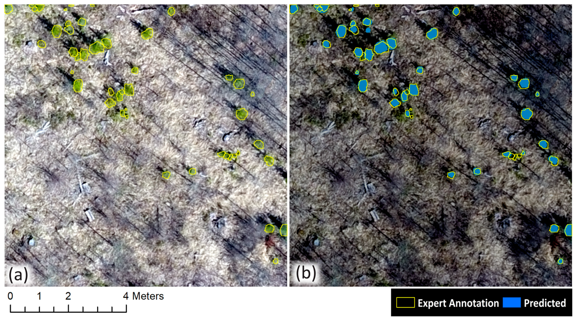
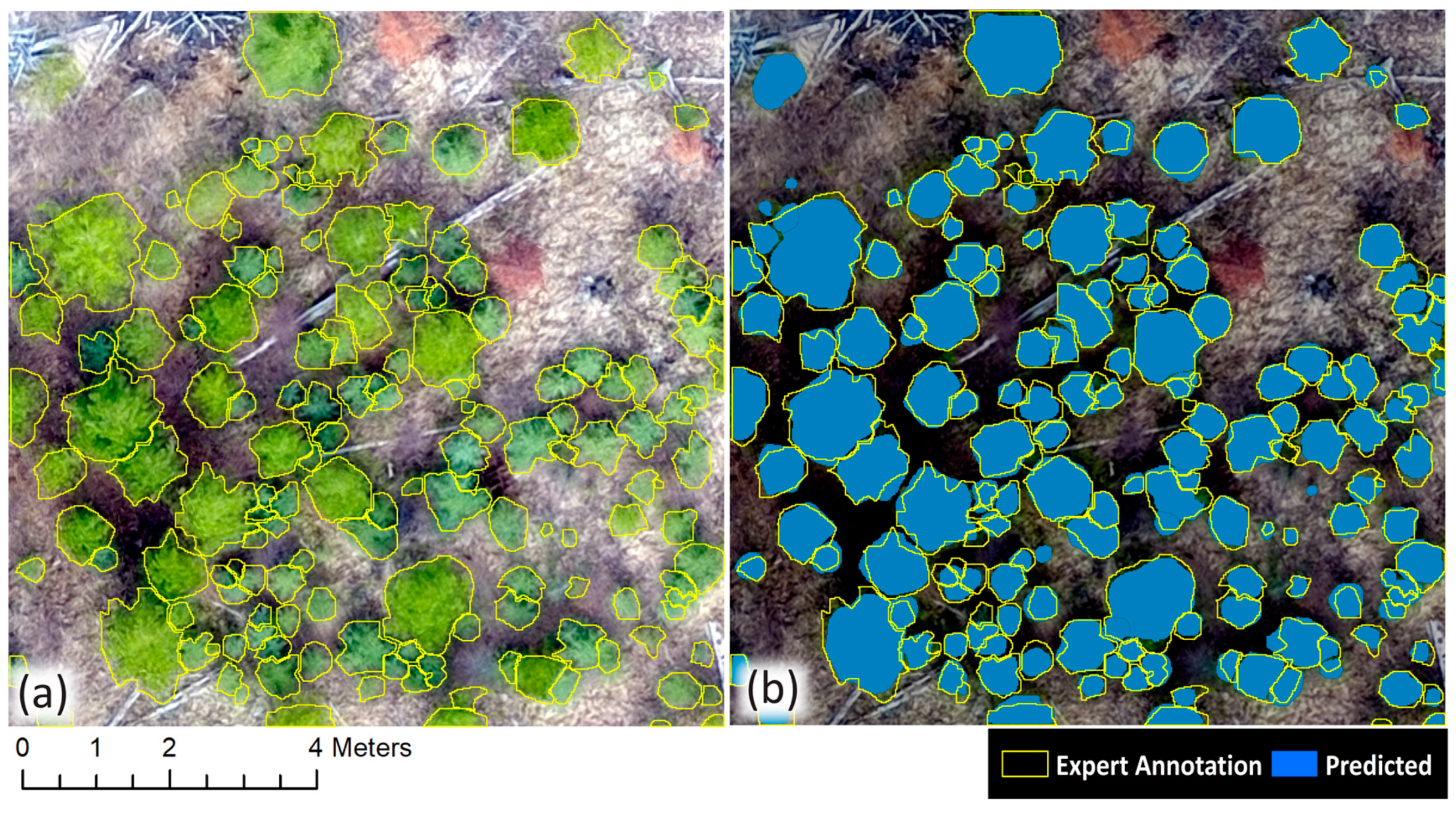
In this study, working in regenerating stands 12–14 years postharvest, we assess the ability of Mask R-CNN to delineate individual coniferous trees in imagery collected during the early spring, before deciduous green-up (leaf-off conditions). We then extract height information from DAP-derived CHM and compare the results to reference data collected in the field. To do so, we first train Mask-R-CNN to automatically delineate regeneration crowns using UAV-acquired RGB imagery. We assess the efficacy of this approach across a range of regenerating stands of different boreal forest types and growing conditions in managed forests in west-central Alberta, Canada. We then explore the potential to use predicted ITC polygons to automatically extract tree-level height information from a DAP-generated CHM. This research serves as a contribution towards the goal of automating regeneration monitoring using remote sensing techniques.

2. Materials and Methods

2.1. Study Sites

Eighteen regenerating stands in the Drayton Valley and Rocky Mountain House regions of Alberta, Canada, were selected, representing 7 of the 10 typical stand types in Alberta [37] (

Table 1. Summary information for each of the 18 regenerating stands selected as study sites.

Site	ForestType	Density (Stems/ha)	Area (ha)	Primary Species	Secondary Species	Tertiary Species
B19	Pine (Pl)	2800	9.2	Lodgepole pine	White spruce	Aspen
B20	White spruce (Sw)	1700	17.3	White spruce	Lodgepole pine	Aspen
B21	Hardwood-Spruce (HwSx)	5500	6.5	Aspen	White spruce	White birch
B22	Hardwood-Pine (HwPl)	7000	6.6	Aspen	Balsam poplar	White birch
B28	Pine-Hardwood (PlHw)	5800	10.9	Lodgepole pine	Aspen
B29	Hardwood-Pine (HwPl)	6000	6.9	Aspen	Lodgepole pine
B32	White Spruce (Sw)	1500	6.5	White spruce
B33	Hardwood (Hw)	6800	2.8	Aspen	White spruce	Lodgepole pine
B34	Pine (Pl)	6400	13.4	Lodgepole pine
B35	Pine (Pl)	3800	5.3	Lodgepole pine
B38	Hardwood-Spruce (HwSx)	5400	12.5	Aspen	White spruce	Balsam poplar
B39	White Spruce (Sw)	1700	2.7	White spruce	Lodgepole pine	Aspen
B41	White Spruce-Hardwood (SwHw)	2800	8.7	White spruce	Aspen	White birch
B43	White Spruce-Hardwood (SwHw)	3200	14	White spruce	Aspen	Balsam poplar
B49	White Spruce-Hardwood (SwHw)	3400	2.2	White spruce	Aspen
B51	Pine-Hardwood (PlHw)	3400	12	Lodgepole pine	Aspen	White spruce
B54	Hardwood-Pine (HwPl)	5400	24.6	Aspen	Lodgepole pine	White spruce
B57	Hardwood-Spruce (HwSx)	5400	24.5	Aspen	White spruce	Lodgepole pine

, Figure 1). Dominant species were lodgepole pine (Pinus contorta), white spruce (Picea glauca), and aspen (Populus tremuloides). Balsam poplar (Populus balsamifera), white birch (Betula papyrifera), and black spruce (Picea mariana) were also present. These stands are typical of other stands of similar types across the province because: (1) forest companies are required by law to create the stand type that was harvested; and (2) all stands across the province are required to meet the same base 10 stratum specific minimum stocking standard based on a minimum tree height requirement [2].

Four of the selected stands are located in the Upper Foothills Natural Subregion with the remaining fourteen being located in the Lower Foothills Natural Subregion. All sites were within 50 km of each other. The Upper Foothills Natural Subregion is characterized by conifer and mixed conifer stands while the Lower Foothills Natural Subregion is characterized by codominance of conifer (lodgepole pine, white spruce, black spruce) and deciduous (aspen, balsam poplar, white birch) stands [38]. These stands and tree species represent five of the seven commercial tree species harvested in Alberta. The Lower Foothills Natural Subregion represents a transition from the aspen-white spruce dominated forests of the Central Mixedwoods Natural Subregion and the lodgepole pine dominated forests of the Upper Foothills Natural Subregion. Topography is generally rolling (morainal deposits) in the Lower Foothills Natural Subregion and strongly rolling in the Upper Foothills Natural Subregion [38]. However, most of the selected stands displayed mild slopes.

2.2. Field Measurements

To meet the regulatory requirements of the Reforestation Standard of Alberta, each stand was visited by a trained field crew in the fall of 2017. Circular plots (10 m²) were established using a systematic sampling design, with the number of plots proportional to the size of each sampled stand. At each plot location, trees were tallied by species. In addition, at every 4th plot a larger 100 m² circular plot was also established with the same center. At each larger plot location, top height trees (largest diameter trees at breast height by Aw, Pl, Sw, and Sb tree species groups) were identified by trees species and measured for total height and total age for site index determination. Plots were spatially located using a Garmin GPSMAP 64s device and height measurements were taken with a Vertex hypsometer.

In the spring of 2018 prior to bud flush, plot centers sharing both the small and large plot were relocated and marked with spray paint. Height and species data were verified for trees within each plot. Measured top height trees were marked with a spray paint halo to ensure visibility in the imagery. Azimuth and distance from plot center for top height trees were also recorded. Once the plots were marked and measured, imagery was collected. Measured trees were then related to corresponding orthomosiacs using their azimuth and distance to plot centers. During this step, some points required manual adjustments and fifteen field-measured conifers could not be located in orthomosaics with certainty. Of the remaining 214 field-measured conifers that were located, 76 were lodgepole pine and 138 were white spruce. Mean height was 3.41 m and 2.31 m with a range of 6.1 m and 5.0 m for lodgepole pine and white spruce, respectively.

2.3. Imagery Acquisition

2.3.1. Leaf-Off Conditions

Imagery was acquired in early spring after snow-melt but before deciduous green-up had occurred. At this time of year, deciduous trees were leafless and grasses were still dormant and therefore light brown in color. Hence, under these leaf-off conditions, conifers (lodgepole pine and white spruce) were almost exclusively the only source of green reflectance (some patches of green moss were present). Furthermore, conifers situated beneath deciduous overstorey, which would otherwise be obscured during periods of deciduous foliage, were visible under leaf-off conditions.

2.3.2. Acquisition Parameters

True colour RGB imagery was acquired with a DJI Phantom 4 pro quadcopter over a 6-day period in May 2018. Imagery was acquired with a 20-megapixel 1” CMOS sensor. Prior to flights, at least three 60 × 60 cm targets (bicolor panels) were evenly distributed throughout each site. The location of the center point of each target was measured utilizing a Trimble Geo7× to produce high-accuracy ground control point coordinates (

Table 2. Input UAV imagery, ground control point counts with mean root mean square error (RMSE), and output point density (mean and standard deviation) for each of the eighteen stands. Mean point density was calculated by sampling ten 50 m² plots, which were evenly distributed throughout each site.

Site	Images		Ground Control Points		Density (pts/m2)
	Calibrated	Total	Count	Mean RMSE (m)
B19	551	575	4	0.034	2654 ± 249.4
B20	725	725	5	0.057	2956.7 ± 352.9
B21	476	477	4	0.039	2733.4 ± 211.9
B22	645	645	6	0.071	2727.7 ± 255.2
B28	456	456	4	0.033	2974.2 ± 449.8
B29	535	535	4	0.11	2699.4 ± 687.6
B32	296	296	3	0.042	2667 ± 193.8
B33	149	149	3	0.117	2248.5 ± 129.1
B34	755	757	2	0.001	2717.5 ± 351.6
B35	387	387	4	0.074	2656.1 ± 351.8
B38	651	651	2	0.001	3043.7 ± 642.1
B39	137	137	3	0.038	2359.8 ± 202.6
B41	996	996	4	0.047	2841.9 ± 284.8
B43	738	738	4	0.024	3017.8 ± 375.3
B49	122	122	3	0.086	2316.4 ± 348.3
B51	477	477	3	0.055	2684.2 ± 348.7
B54	1720	1730	5	0.132	2297.4 ± 200.6
B57	1204	1205	5	0.089	3374.7 ± 328.1

). Flight patterns were programmed to achieve approximately 85% and 80% along- and across-track overlap, respectively. Flights were 100 m above ground level. Ground sampling distance (GSD) was approximately 3 cm. Flights occurred throughout the day under mostly clear sky conditions with minimal wind.

2.4. Point Cloud Processing

UAV imagery was georeferenced using ground control point locations prior to the construction of DAP point clouds and orthomosaics with Pix4D software [39]. After tie-point pixels between overlapping imagery were matched, DAP point clouds were produced and 3-band (RGB) orthomosaics were exported. DAP point clouds were processed in LAStools [40] where they were classified into ground or nonground points. Points with maximum height values were used to construct digital surface models. Ground points were used to construct digital terrain models. Canopy height models (CHM) with a 3 cm resolution were then created according to the methods detailed by Khosravipour et al. [36]. DAP processing took approximately 3.5 h per hectare of imagery.

For processing within Mask R-CNN (described below), we subset the 3-band (RGB) orthomosaics into 600 × 600-pixel image tiles derived by splitting said orthomosaics with a 20% overlap (120 pixels in all directions). Orthomosaics were subset with overlap to account for trees that may be occluded by image tile boundaries, ensuring that all trees were fully visible in at least one image tile.

2.5. Training and Validation Data

One hundred and ten subset image tiles were selected for manual annotation, during which ITC were delineated as polygons. Fifty-two percent of these image tiles were from stands in which lodgepole pine were the dominant coniferous species. Remaining image tiles contained dominant stands of white spruce. Manually annotated subset image tiles were verified by a qualified Alberta Vegetation Inventory Level II interpreter. Figure 2 provides examples of these manually annotated subset image tiles. The 110 tiles were divided into 88 training tiles, 11 internal validation tiles, and 11 external validation tiles, following a 80:10:10 ratio [29].

2.6. Mask R-CNN

In the following section, we provide a high-level explanation of our Mask R-CNN approach for this study and refer readers to He et al. [41] for a more detailed background to the approach.

2.6.1. The Learning Process

The learning process for Mask R-CNN consists of two phases: training and validation [24]. During the training phase, Mask R-CNN applies a succession of convolutional filters to input imagery with the goal of distinguishing target ITC from background features [41]. The validation phase then tests filter combinations on examples that Mask R-CNN has not yet been exposed to—the internal validation set [24]. During the validation phase, Mask R-CNN will score its ability to delineate ITC using the filter combinations developed during the training phase and subsequently determine a new configuration of convolutional filters that are likely to yield a higher score. The training and validation phases are then repeated across the entire training and internal validation datasets. Each repetition of the training and validation phases is called an epoch and the total number of epochs Mask R-CNN performs is dictated by the user. Following the completion of an epoch, we accessed Mask R-CNN’s performance on the external validation set, using average F1 score (described in Section 2.7) as a determinant of success.

2.6.2. Pretrained Networks

Previous studies have shown that initializing training using a pretrained CNN (transfer learning) reduced the duration of training time and subsequently improved results [17,18,42]. One key dataset that has been widely used to pretrain CNN across a variety of applications is the Microsoft Common Objects in Context (hereby referred to as MS COCO) dataset [43], which contains upwards of 91 object types (“Dog”, “Person”, “Plane”, etc.). While a new model may not be trained to identify these object classes, the low-level features a CNN is trained to detect, including edges, textures, and simple geometry, are components of all objects and thus, transfer learning has demonstrated the ability of CNN to repurpose low-level features for the semantic segmentation of new object classes [17]. As demonstrated by Hu et al. [44] and Zhao, et al. [17], initializing training on remotely sensed imagery using a CNN pretrained with natural imagery improved results. Likewise, Fromm et al. [18] found pretraining to positively influence the performance of Faster R-CNN, a progenitor of Mask R-CNN.

We trained Mask R-CNN in separate instances using two Mask R-CNN models that were pretrained on different versions of the MS COCO dataset. The first pretrained network (hereby referred to as COCO), like many, was trained on the MS COCO dataset as presented by [43]. The second pretrained network (hereby referred to as Balloon) was trained on an expanded version of the MS COCO dataset that included a new object class for the semantic segmentation of individual and overlapping balloons in natural imagery [24]. We hypothesized that the similarities between the roughly circular footprints of our target conifer ITC and those of balloons would pose an advantage for the Balloon pretrained network over the COCO pretrained network.

2.6.3. Training Strategy

The architecture of Mask R-CNN is comprised of two main components: the network backbone and the network heads [25]. The backbone consists of convolutional layers used for feature extraction, while the heads consist of convolutional layers used for mask and bounding box prediction [25]. During the learning process, convolutional filters of the backbone or heads can be separately adjusted or frozen [24]. Because the backbone of a pretrained network is already trained to extract object features, it may not be necessary to adjust the backbone and adjusting only the heads will suffice to adapt to a new task [17]. However, allowing for the network’s backbone and heads to be adjusted simultaneously can facilitate the learning of new features which will allow for Mask R-CNN to better solve a new task [17].

We investigated in separate instances (1) adjusting only network heads and (2) adjusting the heads and backbone simultaneously (all layers), where the first training strategy would elucidate the transferability of pretrained features and the second would demonstrate whether performance improvements could be made if the entire network were adjusted to solve our problem. In all instances, performance on the external validation set plateaued before 60 epochs had elapsed. Each epoch took approximately 18 min using a NVIDIA Quadro M4000 GPU.

2.6.4. Hyperparameter Changes

While repurposing a pretrained network is likely to improve results, some hyperparameters may need to be adjusted to account for differences between applications. For example, in order to adapt a version of Mask R-CNN pretrained with COCO to detect nuclei in medical imagery, Waleed [24] needed to account for differences between images in each dataset. Namely, images in the MS COCO dataset contained fewer object instances than did images in the nucleus dataset. Objects in the MS COCO dataset were generally larger than those in the nucleus dataset. To account for this, Waleed [24] increased the maximum number of object instances utilized per image during training from 100 to 200 and increased the maximum number of final detections from the default of 100 to 400. Additionally, to increase the number of detections, the non-maximum suppression threshold for the region proposal network was increased from 0.7 to 0.9, which increased the likelihood of detecting all nuclei in a given image.

In this research, the maximum number of detections was set to 300 on the assumption that training image tiles contain between approximately 1 and 250 delineated trees. The threshold for the number of ground truth instances used during training was set to 300 to ensure that all delineated trees within an image tile were used. To increase the number of proposals and detections during training, the region proposal network’s non-maximum suppression threshold was set to 0.9 following [24]. The number of post non-maximum suppression regions of interest was set to 2000 to increase the number of opportunities for Mask R-CNN to make positive detections (especially in images with many densely clustered ITC). The minimum acceptable detection confidence was set to 0.5 to reduce the likelihood of incurring false negatives for small ITC that blend in with the background. Additionally, we used the Adaptive Moment Estimation (Adam) optimization algorithm, which has seen extensive use in CNN applications and has been recommended as the best general option for optimization algorithms [45].

2.6.5. Image Augmentation

To reduce the impact of overfitting these parameters on small training datasets, image augmentation in the form of simple geometric transitions, including flipping and rotating input training data, have been employed to expose CNN to statistically different examples of their assigned target objects [18,42]. Likewise, blurring images and altering their brightness can improve the robustness of a neural network towards radiometric variation between images [29]. For this research, we used the default Mask R-CNN image augmentation routine. This included blurring original images and altering their brightness in addition to performing random vertical and horizontal flips, and 90-, 180-, and 270- degree rotations. Each time Mask R-CNN loaded an image during training, it performed zero to two of these image augmentations.

2.7. Model Evaluation

To quantify agreement between predicted ITC delineations and ground truth ITC, we used intersection over union (IoU), which is calculated as the number of pixels shared between predicted ITC and ground truth ITC divided by the total number of pixels contained in both entities [18] (Equation (1)). We considered a predicted ITC to be a true positive (TP) when the IoU value was greater than or equal to 0.5.

$$\mathrm{IoU}=\frac{\mathrm{Predicted}{\displaystyle \cap }\mathrm{Ground}\mathrm{Truth}}{\mathrm{Predicted}{\displaystyle \cup }\mathrm{Ground}\mathrm{Truth}}$$

(1)

We calculated precision, recall, and F1 score at an IoU threshold of 0.5 for each image tile in the external validation set. Precision is the percentage of predicted ITC that were deemed true positives, and recall is the percentage of ground truth ITC that were correctly predicted. F1 Score is the harmonic mean of precision and recall, which we used as an indicator of overall accuracy [46]. Precision, recall, and F1 score values range from zero to one, where higher values indicate better results.

To facilitate comparison between models, we calculated average precision (AP) and average recall (AR) for all image tiles in the external validation set. We then calculated the average F1 score for each model as the harmonic mean of AP and AR.

$$\mathrm{Precision}=\frac{\mathrm{True}\mathrm{Positive}}{\mathrm{True}\mathrm{Positive}+\mathrm{False}\mathrm{Positive}}$$

(2)

$$\mathrm{Recall}=\frac{\mathrm{True}\mathrm{Positive}}{\mathrm{True}\mathrm{Positive}+\mathrm{False}\mathrm{Negative}}$$

(3)

$$\mathrm{F}1\mathrm{Score}=2\ast \frac{\mathrm{Precision}\ast \mathrm{Recall}}{\mathrm{Precision}+\mathrm{Recall}}$$

(4)

2.8. Height Extraction and Comparison to Field Measurements

Following model evaluation, we applied our best-performing model to delineate ITC in each stand, using overlapping image tiles as input. We employed an automated postprocessing routine to eliminate redundant ITC polygons generated from predictions made on overlapping input image tiles. ITC polygons located within the 20% overlap zone of each output tile were labeled and shrunk to minimize the number of ITC polygons with shared borders. ITC polygons that overlapped after shrinkage were merged, thereby eliminating redundant or partial ITC polygons generated from overlapping input image tiles and unifying output tiles for each study site as single shapefile spanning the extent of that site. The maximum CHM value within each ITC polygon was then appended as an attribute. Predicted ITC within the surveyed plots were visually inspected. Those ITC that encompassed field-measured tree locations were deemed correct detections. Field-measured and CHM-extracted height measurements for detected ITCs were then compared by simple linear regression.

CHM-extracted height measurement error was quantified using Equations (5)–(7). Error was calculated as remote height minus field height (Equation (5)) so as to indicate over- and underestimation with positive and negative error values, respectively. Because error values were inherently smaller for shorter conifers, unsigned relative error (Equation (7)) was used to express discrepancies between field and remote height measurements as a percentage of field height, which required the calculated of unsigned error (Equation (6)).

$$\mathrm{Error}={\mathrm{Height}}_{\mathrm{remote}}-{\mathrm{Height}}_{\mathrm{field}}$$

(5)

$$\mathrm{Unsigned}\mathrm{Error}=\sqrt{{\mathrm{Error}}^2}$$

(6)

$$\mathrm{Unsigned}\mathrm{Relative}\mathrm{Error}=\frac{\mathrm{Unsigned}\mathrm{Error}}{{\mathrm{Height}}_{\mathrm{field}}}\times 100$$

(7)

3. Results

3.1. Mask R-CNN

When only the network heads were adjusted during training, the performance of the Balloon pretrained network plateaued at epoch 27 (Figure 3a). The COCO pretrained network plateaued at epoch 34. Despite the extended training period of the COCO pretrained network, its average F1 score was approximately 0.12 less than that of the Balloon pretrained network (

Table 3. Average precision, recall, and F1 score values for instances of Mask R-CNN trained under different parameters. Column 1 lists the network layers adjusted during training and Column 2 lists the pretrained network with which training was initialized. The average F1 score as weighted by the number of total trees is also included for reference.

Layers Trained	Pretrained Network	Average Precision	Average Recall	Average F1	Tree-Weighted Average F1
Heads	Balloon	0.99	0.76	0.85	0.84
Heads	COCO	0.98	0.61	0.73	0.71
All	Balloon	0.98	0.85	0.91	0.90
All	COCO	0.99	0.81	0.89	0.88

). These factors support our hypothesis that the features learned by the Balloon pretrained network were more transferable to solving the task of ITC delineation.

When all network layers (heads + backbone) were adjusted during training, the impact of the selected pretrained networks on performance was minimal (Figure 3b, Table 3). The Balloon pretrained network plateaued at epoch 45 with an average F1 score of 0.91 and the COCO pretrained network plateaued at epoch 47 with an average F1 score of 0.89. Both of these F1 scores were greater than any of those yielded by training only the network heads.

3.1.1. Individual External Validation Tiles

Differences between the Balloon and COCO pretrained networks where all layers were adjusted during training were more pronounced for some individual external validation tiles than others. These external validation tiles are shown in Figure 4 with each tile name corresponding to the items in the first column of Table 3 and

Table 4. Evaluation metrics for the instance of Mask R-CNN trained with the Balloon pretrained network where all layers were adjusted during training. TP = true positive; FP = false positive; FN = false negative.

Tile	Total Trees	TP	FP	FN	Precision	Recall	F1
a	97	85	1	12	0.99	0.88	0.93
b	46	32	1	14	0.97	0.7	0.81
c	81	69	0	12	1	0.85	0.92
d	157	127	5	30	0.96	0.81	0.88
e	92	71	1	21	0.99	0.77	0.87
f	79	71	2	8	0.97	0.9	0.93
g	48	46	0	2	1	0.96	0.98
h	15	13	0	2	1	0.87	0.93
i	109	88	0	21	1	0.81	0.89
j	16	14	0	2	1	0.88	0.93
k	44	39	2	5	0.95	0.89	0.92

. Generally, the Balloon pretrained network yielded more TP at the cost of a slight increase in FP (Table 4 and

Table 5. Evaluation metrics for the instance of Mask R-CNN trained with the COCO pretrained network where all layers were adjusted during training. TP = true positive; FP = false positive; FN = false negative.

Tile	Total Trees	TP	FP	FN	Precision	Recall	F1
a	97	85	1	12	0.99	0.88	0.93
b	46	29	0	17	1	0.63	0.77
c	81	62	0	19	1	0.77	0.87
d	157	122	2	35	0.98	0.78	0.87
e	92	63	0	29	1	0.68	0.81
f	79	67	2	12	0.97	0.85	0.91
g	48	47	0	1	1	0.98	0.99
h	15	12	0	3	1	0.8	0.89
i	109	86	0	23	1	0.79	0.88
j	16	14	0	2	1	0.88	0.93
k	44	41	0	3	1	0.93	0.96

). This was true for all external validation tiles except for tiles g and k, where the COCO pretrained network yielded slightly more TP. The greatest difference in F1 score was observed for tile e (+0.06 for the Balloon pretrained network).

In the following subsections, we highlight as case studies the performance of the Balloon pretrained network (trained with all layers) on four external validation tiles. Delineation results and expert annotations (ground truth data) are visualized alongside their corresponding image tile in Figure 5, Figure 6, Figure 7 and Figure 8. In Panel (b) of these figures, the original image tile has been darkened to contrast the predicted ITC.

Mean crown area, mean inter-crown distance, and mean IoU between predicted and interpreted ITC are also provided to aid the reader in characterizing each case study (

Table 6. Descriptive metrics for the external validation tiles discussed in Case Study 1–4.

Case Study	Tile	Mean Crown Area (m2)		Mean Crown Distance (m)		Mean IoU	Total Trees
		Predicted	Annotated	Predicted	Annotated
1	b	0.23	0.17	0.50	0.35	0.68	46
2	d	0.81	0.75	0.09	0.07	0.70	157
3	e	0.33	0.30	0.41	0.42	0.69	92
4	g	0.64	0.63	0.80	0.80	0.81	48

). Each of these case studies are representative of various conditions found across all training and validation data, which are discussed in detail below.

3.1.2. Case Study 1: External Validation Tile b (B21)

Tile b is representative of the smallest ITC found in all training and validation tiles. Tile b yielded the lowest F1 and recall scores among all external validation tiles. Mean crown area was 0.23 m² and 0.17 m² for predicted and annotated ITC, respectively (Table 6). The mean inter-crown distance was 0.50 m and 0.35 m for predicted and annotated ITC, respectively. Predicted ITC in Tile b displayed the worst fit to interpreted mean crown area and annotated mean inter-crown distance. However, both the annotated mean crown area and predicted mean crown area also were lowest found in any external validation tile.

3.1.3. Case Study 2: External Validation Tile d (B29)

Tile d was the densest external validation tile with respect to tree crowns, with the highest number of total trees (157) and the lowest mean inter-crown distance. Similar conditions are found in Tile i, which exhibits clustered crowns and a high number of total trees. Localized clustering of crowns of varying sizes is also found in Tile c. Tile d contained both the highest number of FP and the highest number of FN. Tile d yielded the second lowest mean IoU between predicted and annotated ITC. The mean inter-crown distance was 0.09 m and 0.07 m for predicted and annotated ITC, respectively. Mean crown area was 0.81 m² and 0.75 m² for predicted and annotated ITC, respectively (Table 6).

3.1.4. Case Study 3: External Validation Tile e (B33)

Tile e is representative of the shading and obscuration by adjacent deciduous trees found in hard- and mixed-wood forests. This tile contains the lowest mean IoU between predicted and annotated ITC as well as the second lowest F1 and recall scores among all external validation tiles. External validation tiles, j and h display similar deciduous forest components. However, Tile j and Tile h contain fewer total trees and contain ITC that are more dispersed than those found in Tile e.

3.1.5. Case Study 4: External Validation Tile g (B39)

Tile g yielded the highest F1 and recall scores as well as the greatest mean IoU between predicted and annotated ITC among all external validation tiles. The mean inter-crown distance was 0.80 m for both predicted and annotated ITC. Mean crown area was 0.64 m² and 0.63 m² for predicted and annotated ITC, respectively. Tile g displayed the closest fit to annotated mean crown area. External validation tiles, a and k, exhibit similar conditions as those found in Tile g, with Tile a containing more total trees and higher global clustering, and Tile k containing fewer total trees, which are more dispersed than those found in Tile a or Tile g.

3.2. Height Extraction and Comparison to Field Measurements

Of the 214 field-measured conifers, 90.6% were detected (

Table 7. Count and summary information for 194 field-measured conifers. The best-performing version of Mask R-CNN (Balloon pretrained network where all layers were adjusted during training) was applied to delineate 214 conifers that were measured in the field. Ten of these conifers were not detected. Of the detected field-measured conifers, there were approximately two white spruce for each lodgepole pine.

Forest Type	Stands Sampled	Detected Conifers	Conifer Species
			White Spruce	Lodgepole Pine
Hw	2	26	12	14
HwPl	2	17	9	8
HwSx	3	32	25	7
Pl	3	37	16	21
PlHw	2	26	15	11
Sw	3	30	27	3
SwHw	3	26	23	3
Total	18	194	127	67

).

Mean error, unsigned error, and unsigned relative error were −0.33 m, 0.42 m, and 20%, respectively for all field-measured conifers (

Table 8. Descriptive statistics for each error type. While the mean and median values of lodgepole pine are more desirable than those of white spruce, the lodgepole pine error distributions are less consistent with the exception of unsigned relative error.

	Species	Mean	Median	Std	Range
Error (m)	Both	−0.33	−0.36	0.36	1.79
	White Spruce	−0.37	−0.38	0.32	1.62
	Lodgepole Pine	−0.24	−0.22	0.41	1.79
Unsigned Error (m)	Both	0.42	0.39	0.25	1.08
	White Spruce	0.44	0.40	0.22	0.89
	Lodgepole Pine	0.37	0.33	0.29	1.08
Unsigned Relative Error (%)	Both	20	17	15	76
	White Spruce	24	19	15	75
	Lodgepole Pine	13	10	12	50

). Thirty-two DAP-derived height measurements overestimated their corresponding field measurements, with the remaining 162 being underestimated. Mean unsigned error was 0.27 m and 0.45 m for overestimated and underestimated trees, respectively. Mean unsigned relative error was 11% and 22% for overestimated and underestimated trees, respectively.

A simple linear regression (r² = 0.93, RMSE = 0.34 m) revealed that field and remote height measurements were highly correlated (Figure 9). Furthermore, the line of best fit runs nearly parallel to that of the 1:1 line, revealing a systematic trend of height underestimation (Figure 9).

3.2.1. Species

Median error was closer to zero for lodgepole pine individuals than it was for white spruce individuals across all height classes (Figure 10a). However, lodgepole pine error was less consistent than white spruce error, which is demonstrated by greater interquartile ranges for lodgepole pine across all height classes (Figure 10a). The 1st and 3nd height classes contained the closest median error values to zero for white spruce and lodgepole pine, respectively (Figure 10a). The difference in median error between the lodgepole pine and white spruce distributions was greatest at the 5th height class interval (>4 m) (Figure 10a). Median lodgepole pine error undulated across all height class intervals it appeared in, whereas median white spruce error became increasingly distant from zero between the 1st and 5th height class intervals (<1 m to >4 m) (Figure 10a). Unsigned relative error was greatest for conifers beneath 2 m in height (Figure 10b). As with error in Figure 10a, the difference in median unsigned relative error between the white spruce and lodgepole pine distributions was greatest at the 5th height class interval (Figure 10b).

3.2.2. Forest Type

Median values for white spruce error distributions are clustered between approximately −0.5 m and −0.3 m, with the highest and lowest median values coming from PlHw and SwHw stands, respectively (Figure 11a). Error and unsigned relative error distributions for white spruce sampled from SwHw stands have the most variation for this species (Figure 11). The greatest median unsigned relative error values for white spruce came from Hw, HwPl, SwHw, and PlHw stands (in descending order) (Figure 11). The Hw unsigned relative error distribution has the highest minimum, maximum, and median values for white spruce (Figure 11b). For lodgepole pine, those sampled from Hw stands had the furthest median error value from zero (Figure 11a). Error distributions for lodgepole pine sampled from Pl stands have the most variation for this species (Figure 11a). Unlike with white spruce, the forest type associated with the greatest variation in unsigned relative error for lodgepole pine (HwSx) is not the same as the forest type associated with the greatest variation in error (Pl) (Figure 11).

4. Discussion

4.1. ITC Delineation

Due to the scarcity of recent studies on the delineation of regenerating, as opposed to mature, conifer crowns, in this section, we draw on literature pertaining to ITC detection and delineation in various forest types of various ages for comparison to our research. To facilitate comparison to studies reporting detection rates as a percentage, we calculate our delineation accuracy as the total number of TP divided by the total number of annotated reference trees (83.5%) and we use average F1 score for comparison with other studies using CNN for ITC delineation. All studies hereafter mentioned in this section were carried out in mature forests or plantations, except for [19,47]. Generally speaking, increasingly heterogeneous forest conditions (age, species, etc.) will have a negative effect on detection and delineation accuracy and the results reviewed in this section should be interpreted with this in mind. The stands sampled in this study were managed sites following harvest. They were approximately 14 years in age with crowns much smaller than those found in mature forests (approximately 42% of field-measured trees had crown diameters less than one metre and 93% were below two metres). With regard to spacing and age, conditions ranged from open, evenly spaced and evenly aged crowns (similar to a planation), to dense, clustered and overlapping crowns of mixed ages.

In the context of natural regeneration in a Norway spruce dominant forest, Röder et al. [47] detected individual trees with a success rate of 39.1% using a local maxima-based approach. Yancho et al. [48] achieved 47.6% detection accuracy with a subcrown point clustering approach applied in a mature, coniferous dominant, temperate rainforest. In a mature, mixed-wood forest, Berra [49] yielded overall accuracies as high as 80% for the delineation of coniferous trees in plots containing approximately 40 trees using a watershed-based approach. In plantation settings, Kattenborn et al. [50] and Torres-Sánchez et al. [51] yielded overall accuracies of 86% and 90%, respectively for ITC delineation with object-based image analysis (OBIA) approaches.

Weinstein et al. [52] applied a semi-supervised CNN approach to detect ITC in an open woodland in central California, achieving an F1 score of 0.65. In a complex, tropical forest, Braga et al. [32] achieved an F1 score of 0.86 using a Mask R-CNN-based workflow to delineate ITC. Li et al. [53] achieved an F1 score of 0.95 using a CNN approach to delineate ITC in a palm oil plantation. Finally, Pearse et al. [19] achieved F1 scores of approximately 0.99 and 0.98 for the detection of coniferous seedlings in two regeneration trials in New Zealand using a Faster-RCNN architecture. Detection was carried out on RGB imagery with an approximate GSD of 1 cm, in which seedlings size and density was mostly uniform [19].

Despite the heterogeneity of our study sites, our results are comparable to those of Pearse et al. [19], demonstrating the feasibility of the proposed methods for operational delineation of ITC in regenerating boreal forests. However, small, and clustered ITC—challenges of past studies [5,9,10,54]—remain contemporary challenges as well [47]. Heterogeneity in crown size and spacing proved to be challenges for this research, which Röder et al. [47] note as sources of error for their approach to automatic ITC detection. Namely, tightly clustered ITC whose branches overlap were a source of error for our approach to ITC delineation. Juvenile trees tend to grow in tight clumps where multiple seeds had become established in close proximity. This is exemplified in External Validation Tile b, the lowest scoring external validation tile, where several small ITC (area ≤ 0.1 m²) were omitted. Likewise, Mask R-CNN had difficulty delineating all ITC in external validation tiles such as Tile d, where ITC of varying sizes were adjacent and overlapping. Difficulty delineating all ITC in Tile d was compounded by the number of total trees contained in this tile (157). However, given that Tile b and Tile e contained fewer total trees than Tile d and that Mask R-CNN performed better on Tile d, crown size may be considered to pose a greater challenge for our approach to ITC delineation.

4.2. Height

Correlation between field and remote height measurements (r² = 0.93) was comparable to what has been reported by other studies using only optical sensors. Röder et al. [47] and Dandois et al. [55] yielded r² values of 0.75 and 0.86, respectively. In regenerating forests, Castilla et al. [35] reported an r² of 0.67 for the measurement of coniferous seedlings. However, most of the seedlings in this study were less than 1 m in height. Goodbody et al. [34] achieved a Spearman’s r of 0.91, which is comparable to results from Lisein et al. [56] (r² = 0.91) and Puliti et al. [57] (r² = 0.97) who produced remote height measurements with hybrid LiDAR-optical data products in mature forests. Variation between results from mature forests [47,55] and regenerating forests [34] suggests that canopy closure may impede the production of accurate ground models from DAP and in turn, the extraction of accurate remote height measurements. The high r² values of Lisein et al. [56] and Puliti et al. [57] demonstrate the utility of LiDAR data in this regard as only active sensors can penetrate dense canopies to normalize terrain occluded by forest canopy. However, regenerating forests in which canopies have not yet fully closed may be uniquely suited for terrain characterization and remote height extraction by DAP as indicated by the results yielded by Goodbody et al. [34] and this study. With this being said, the remote measurement of small trees is not trivial and as increasingly fine GSD are utilized to measure increasingly small targets, error in photogrammetric reconstruction is likely to affect height estimates [35].

4.2.1. Underestimation: Whorl-Height and Top Height

The majority of field height measurements were underestimated by our remote sensing approach. This discrepancy may be driven by the structure of measured trees. Field measurements were taken from the base of a tree to the top of its terminal leader (annual growth). Leaders are isolated growths that extend vertically from the highest whorl of a tree. They are narrow structures (~1–2 cm wide) and as such, provide limited surface area from which pixels can be extracted during photogrammetric processing. Remote height measurements may therefore correspond to the highest whorl of a tree rather than its leader. This would explain discrepancies between field and remote height measurements for white spruce trees as white spruce leaders are between 0.32 and 0.44 m tall in trees of this age [58] and mean error for white spruce trees was 0.38 m.

Discrepancies between field and remote height measurements are not as easily explained for lodgepole pine trees as their leaders are between 0.20 and 0.40 m in height in trees of this age [59] and mean error for lodgepole pine trees was 0.22 m. However, this may be explained by structural differences between white spruce and lodgepole pine trees. First, the needles of lodgepole pine are approximately 1–2 cm longer than those of white spruce and are more dispersed [60], meaning an average lodgepole pine leader will contain more surface area than an average white spruce leader. Moreover, the branches of lodgepole pine trees arc upwards, growing alongside that tree’s leader, while those of white spruce trees tend to grow outwards on a horizontal plane, perpendicular to their leaders. Therefore, the greatest available surface area towards the top of lodgepole pine trees occurs where top-whorl branches terminate around leader, which is approximately at 2/3 the height of the leader. For a lodgepole pine tree with a leader of 0.40 m height, top-whorl branches will terminate at approximately 0.26 m, which is within 0.04 m of the mean error for lodgepole pine trees in this study.

Additional field measurements and image analysis should be undertaken and include height as measured to the top of a tree’s leader in addition to height as measured to the base of the tallest whorl.

4.2.2. Overestimation: Deciduous and Adjacent Conifers

Thirty-two DAP-derived height measurements overestimated their corresponding field measurements. Of these 32 measurements, 13 overestimated field measurements by greater than 0.3 m. Manual inspection of the ITC polygons from which these height measurements were extracted revealed that the pixel coordinates of maximum CHM values were located in the peripheries of said polygons rather than their approximate centers. These pixels likely fall outside of the actual boundary of the tree crowns they were attributed to and rather, they likely belong to taller, adjacent trees whose crowns overlap those of the field-measured trees (Exemplified in Figure 12 and Figure 13).

Overestimation is exemplified in Figure 12 where the border of a target ITC polygon (yellow) encloses pixels from a neighboring crown, which can be distinguished by its lighter colour. The field height measurement for this tree was 4.18 m and the remote height measurement was 4.88 m. Figure 12b displays the CHM within the polygon delineating this tree, in which two distinct clusters of pixels with high values are visible. The right-hand cluster (2) contains the maximum CHM value (4.88 m) within the polygon and overlaps with the light green pixels of the neighboring crown, while the left-hand cluster (1) is better aligned with the center of the polygon. The greatest CHM value within the left-hand cluster (1) is 4.28 m, which is closer to the field-measured height (4.18 m). This example highlights the sensitivity of our height extraction method to the quality of ITC delineation; when conifers are clustered and overlapping, there is an increased likelihood that a given predicted ITC polygon will contain pixels that belong to an adjacent conifer. If that adjacent conifer is taller than the target conifer, the maximum CHM value extracted from the predicted ITC polygon will correspond with the adjacent conifer rather than the intended target.

Figure 13 provides another example of a conifer whose height was overestimated by our approach. Unlike the previous example, there were no adjacent conifers whose crowns overlapped that of the target ITC polygon (yellow). However, the grey pixels surrounding this polygon belong to a leafless deciduous overstory, which also partially obscures the green response of the conifer in question. The greatest CHM values occur in regions of the polygon where green values are low, which suggests that the maximum CHM value extracted from this polygon should be attributed to the deciduous overstory and not the conifer situated below it (Figure 13b). As such, stands with significant deciduous overstory pose a challenge to our approach to height extraction; predicted ITC polygons for conifers located beneath deciduous overstory are likely to contain overstory pixels whose CHM values will exceed those of the conifers. Therefore, maximum CHM values may provide overestimated remote height measurements in stands with significant deciduous overstory.

4.3. Limitations

Manually delineating ITC is a difficult and time-consuming exercise in photo-interpretation. While our results indicate that our manually delineated datasets were created with adequate fidelity, it is likely that these datasets contain some elements of user error inherent to photo-interpretation. For example, the inclusion of pixels from adjacent conifers in some predicted ITC (discussed in Section 4.2.2.) may indicate that the boundaries of some ITC were drawn too loosely when they were manually delineated and as a consequence, Mask R-CNN may have learned to reproduce this behavior.

Aside from the possibility of interpretation error, the requirement of manually delineated datasets to train CNN is considered to be a major limitation for their use [32]; performance tends to improve relative to the number of samples available to a CNN [18], yet manually delineating these samples is labor-intensive. While it is probable that this study could have benefitted from a larger manually delineated dataset, we had to compromise due to time constraints. However, future studies may circumvent this trade-off as recently, algorithms have been developed that generate large synthetic datasets using a relatively small number of manually annotated samples as input [32,52].

Another limitation stems from the likely discrepancies between what is visible in the UAV imagery and what exists in the field. ITC were manually delineated with high fidelity on the UAV imagery; however, this may also have a degree of interpreter error which highlights the continued need for high quality field data to calibrate these types of models.

4.4. Future Research

While the results of this study are encouraging, additional research is specifically required around issues such as top-height versus whorl-height estimation, reliable species classification for both deciduous and coniferous trees, and the utilization of imagery acquired from piloted aircraft rather than UAV given the large areas of regenerating forest that need to be assessed annually. Investigations into each of these issues are needed to meet Alberta’s regeneration monitoring requirements. The use of CNN to delineate and classify crowns is promising, leaving open the question of whether our methods can be applied to with similar success imagery collected using different platforms.

5. Conclusions

In this study, we have presented a workflow for the automatic delineation of individual conifer crowns in true colour orthomosaics using Mask R-CNN and the subsequent extraction of remote height measurements. Our best model was generated by Balloon pretrained network, where all layers of the network were adjusted during training. This achieved an average precision of 0.98, an average recall of 0.85, and an average F1 score of 0.91. Our results show that Mask R-CNN is capable of automatically delineating individual coniferous crowns in a range of conditions common to western boreal forest regeneration under leaf-off conditions and that these crown delineations can be used to extract height measurements at the individual tree level.

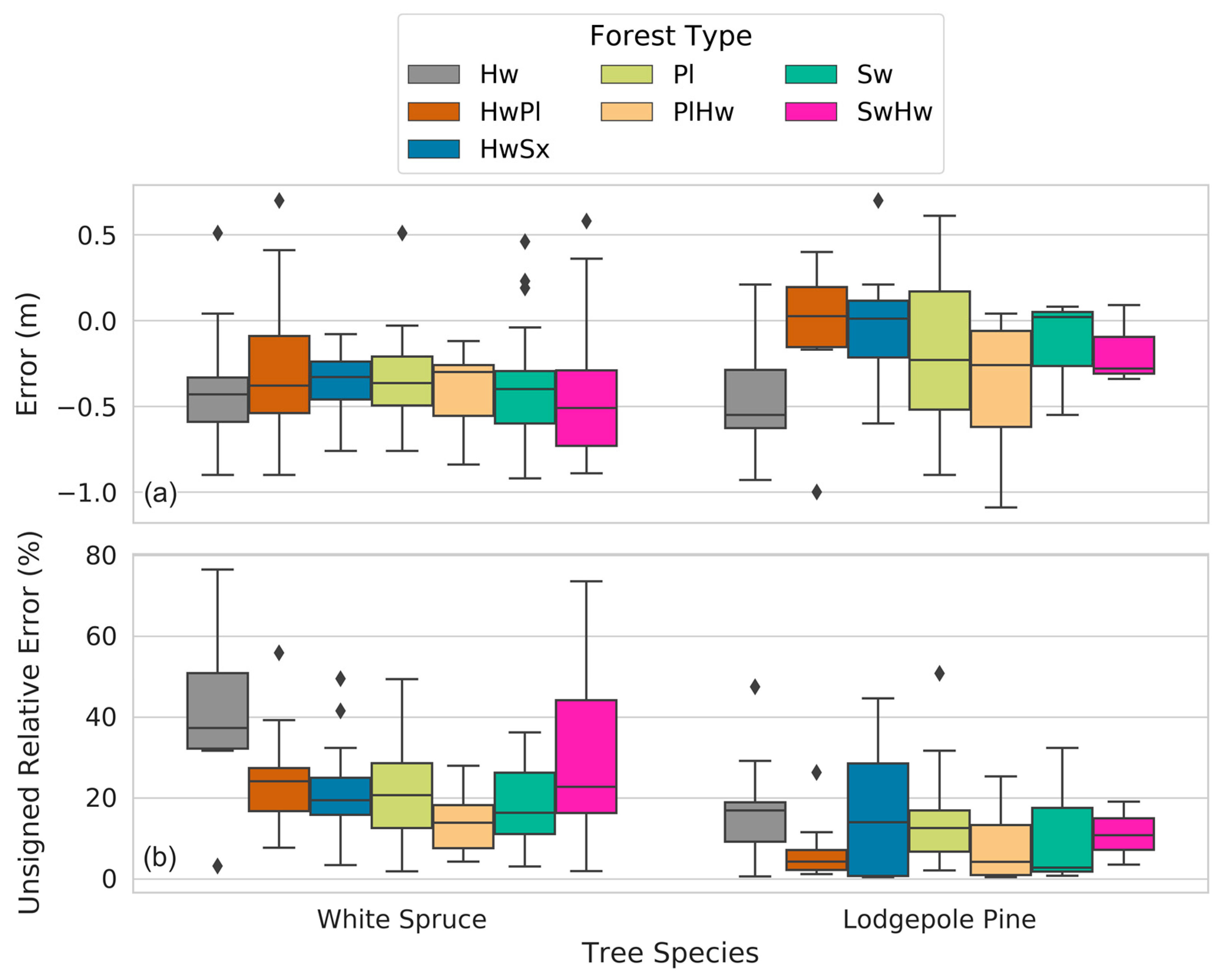
Our height measurement analysis found field and remote height measurements to be highly correlated (r² = 0.93). Remote height measurements tended to underestimate field height measurements (162/194 samples) and mean error was greater for white spruce trees than it was for lodgepole pine (−0.37 m and −0.24 m, respectively). We speculated as to why the majority of remote height measurements underestimated their corresponding field samples as well as why lodgepole pines may be less underestimated than white spruce, and we offered suggestions for future studies to address this challenge. Furthermore, we observed that remote height measurements may overestimate their corresponding field height measurements when a delineated conifer crown contains pixels belonging to taller, adjacent coniferous or deciduous trees.

Our proposed methods to automatically delineate and extract height information for individual conifers in true colour imagery have the potential to improve the speed and scale at which forest regeneration monitoring can occur. However, techniques to classify tree species and delineate individual deciduous crowns from true colour imagery are still required if the criteria of field-based regeneration assessments are to be met by remote sensing approaches. As such, our research serves as a stepping-stone towards the remote automation of regeneration monitoring and future studies should focus on the deciduous components of boreal regeneration as well as the classification of individual tree species.

References

1. Alberta Reforestation Standards Science Council. Linking Regeneration Stands to Growth and Yield and Forest Management Objectives; Sustainable Resource Development (2001–2006, 2006–2013); Alberta Reforestation Standards Science Council: Edmonton, AB, Canada, 2001. [Google Scholar]
2. Alberta Agriculture and Forestry. Reforestation Standard of Alberta; Alberta Agriculture and Forestry: Edmonton, AB, Canada, 2020.
3. Pouliot, D.; King, D.J.; Bell, F.; Pitt, D. Automated tree crown detection and delineation in high-resolution digital camera imagery of coniferous forest regeneration. Remote Sens. Environ. 2002, 82, 322–334. [Google Scholar] [CrossRef]
4. Lieffers, V.J.; Stadt, K.J.; Feng, Z. Free-to-grow regeneration standards are poorly linked to growth of spruce in boreal mixedwoods. For. Chron. 2007, 83, 818–824. [Google Scholar] [CrossRef] [Green Version]
5. Ke, Y.; Quackenbush, L.J. A review of methods for automatic individual tree-crown detection and delineation from passive remote sensing. Int. J. Remote Sens. 2011, 32, 4725–4747. [Google Scholar] [CrossRef]
6. Fassnacht, F.E.; Latifi, H.; Stereńczak, K.; Modzelewska, A.; Lefsky, M.; Waser, L.T.; Straub, C.; Ghosh, A. Review of studies on tree species classification from remotely sensed data. Remote Sens. Environ. 2016, 186, 64–87. [Google Scholar] [CrossRef]
7. Pinz, A. A computer vision system for the recognition of trees in aerial photographs. Multisource Data Integr. Remote Sens. 1991, 3099, 111–124. [Google Scholar]
8. Gougeon, F.A. A Crown-Following Approach to the Automatic Delineation of Individual Tree Crowns in High Spatial Resolution Aerial Images. Can. J. Remote Sens. 2014, 21, 274–284. [Google Scholar] [CrossRef]
9. Gougeon, F.A.; Leckie, D.G. Forest Regeneration: Individual Tree Crown Detection Techniques for Density and Stocking Assessment. Int. J. Remote Sens. 1999, 32, 3625–3647. [Google Scholar] [CrossRef]
10. Gougeon, F.A.; Leckie, D.G. The Individual Tree Crown Approach Applied to Ikonos Images of a Coniferous Plantation Area. Photogramm. Eng. Remote Sens. 2006, 72, 1287–1297. [Google Scholar] [CrossRef]
11. Leckie, D.G. Stand delineation and composition estimation using semi-automated individual tree crown analysis. Remote Sens. Environ. 2003, 85, 355–369. [Google Scholar] [CrossRef]
12. Natesan, S.; Armenakis, C.; Vepakomma, U. Resnet-based tree species classification using uav images. ISPRS Int. Arch. Photogramm. Remote Sens. Spat. Inf. Sci. 2019, 42, 475–481. [Google Scholar] [CrossRef] [Green Version]
13. Cheng, G.; Han, J.; Lu, X. Remote Sensing Image Scene Classification: Benchmark and State of the Art. Proc. IEEE 2017, 105, 1865–1883. [Google Scholar] [CrossRef] [Green Version]
14. Ma, L.; Liu, Y.; Zhang, X.; Ye, Y.; Yin, G.; Johnson, B.A. Deep learning in remote sensing applications: A meta-analysis and review. ISPRS J. Photogramm. Remote Sens. 2019, 152, 166–177. [Google Scholar] [CrossRef]
15. Zhang, L.; Xia, G.-S.; Wu, T.; Lin, L.; Tai, X.C. Deep Learning for Remote Sensing Image Understanding. J. Sensors 2015, 2016, 1–2. [Google Scholar] [CrossRef]
16. Safonova, A.; Tabik, S.; Alcaraz-Segura, D.; Rubtsov, A.; Maglinets, Y.; Herrera, F. Detection of Fir Trees (Abies sibirica) Damaged by the Bark Beetle in Unmanned Aerial Vehicle Images with Deep Learning. Remote Sens. 2019, 11, 643. [Google Scholar] [CrossRef] [Green Version]
17. Zhao, H.; Liu, F.; Zhang, H.; Liang, Z. Convolutional neural network based heterogeneous transfer learning for remote-sensing scene classification. Int. J. Remote Sens. 2019, 40, 8506–8527. [Google Scholar] [CrossRef]
18. Fromm, M.; Schubert, M.; Castilla, G.; Linke, J.; McDermid, G. Automated Detection of Conifer Seedlings in Drone Imagery Using Convolutional Neural Networks. Remote Sens. 2019, 11, 2585. [Google Scholar] [CrossRef] [Green Version]
19. Pearse, G.D.; Tan, A.Y.; Watt, M.S.; Franz, M.O.; Dash, J.P. Detecting and mapping tree seedlings in UAV imagery using convolutional neural networks and field-verified data. ISPRS J. Photogramm. Remote Sens. 2020, 168, 156–169. [Google Scholar] [CrossRef]
20. Fuentes-Pacheco, J.; Olivares, J.L.T.; Roman-Rangel, E.; Cervantes, S.; Juárez-López, P.; Hermosillo-Valadez, J.; Rendon-Mancha, J.M. Fig Plant Segmentation from Aerial Images Using a Deep Convolutional Encoder-Decoder Network. Remote Sens. 2019, 11, 1157. [Google Scholar] [CrossRef] [Green Version]
21. Kentsch, S.; Caceres, M.L.L.; Serrano, D.; Roure, F.; Diez, Y. Computer Vision and Deep Learning Techniques for the Analysis of Drone-Acquired Forest Images, a Transfer Learning Study. Remote Sens. 2020, 12, 1287. [Google Scholar] [CrossRef] [Green Version]
22. Uijlings, J.R.R.; Van De Sande, K.E.A.; Gevers, T.; Smeulders, A.W.M. Selective Search for Object Recognition. Int. J. Comput. Vis. 2013, 104, 154–171. [Google Scholar] [CrossRef] [Green Version]
23. Girshick, R.; Donahue, J.; Darrell, T.; Malik, J. Region-Based Convolutional Networks for Accurate Object Detection and Segmentation. IEEE Trans. Pattern Anal. Mach. Intell. 2015, 38, 142–158. [Google Scholar] [CrossRef] [PubMed]
24. Waleed, A. Mask R-CNN for Object Detection and Instance Segmentation on Keras and TensorFlow. GitHub Repos, 2017. Available online: https://github.com/matterport/Mask_RCNN (accessed on 18 August 2020).
25. He, K.; Gkioxari, G.; Dollar, P.; Girshick, R.B. Mask R-CNN. IEEE Trans. Pattern Anal. Mach. Intell. 2020, 42, 386–397. [Google Scholar] [CrossRef] [PubMed]
26. Johnson, J.W. Adapting Mask-RCNN for Automatic Nucleus Segmentation. arXiv 2018, arXiv:1805.00500. [Google Scholar] [CrossRef] [Green Version]
27. Couteaux, V.; Si-Mohamed, S.; Nempont, O.; Lefevre, T.; Popoff, A.; Pizaine, G.; Villain, N.; Bloch, I.; Cotten, A.; Boussel, L. Automatic knee meniscus tear detection and orientation classification with Mask-RCNN. Diagn. Interv. Imaging 2019, 100, 235–242. [Google Scholar] [CrossRef] [PubMed]
28. Anantharaman, R.; Velazquez, M.; Lee, Y. Utilizing Mask R-CNN for Detection and Segmentation of Oral Diseases. In Proceedings of the 2018 IEEE International Conference on Bioinformatics and Biomedicine (BIBM), Madrid, Spain, 3–6 December 2018; pp. 2197–2204. [Google Scholar]
29. Zhang, W.; Witharana, C.; Liljedahl, A.K.; Kanevskiy, M.Z. Deep Convolutional Neural Networks for Automated Characterization of Arctic Ice-Wedge Polygons in Very High Spatial Resolution Aerial Imagery. Remote Sens. 2018, 10, 1487. [Google Scholar] [CrossRef] [Green Version]
30. Zhao, T.; Yang, Y.; Niu, H.; Chen, Y.; Wang, D. Comparing U-Net convolutional networks with fully convolutional networks in the performances of pomegranate tree canopy segmentation. In Proceedings of the SPIE Asia-Pacific Remote Sensing Conference, Multispectral, Hyperspectral, Ultraspectral Remote Sensing Technology Techniques and Applications VII, Honolulu, HI, USA, 24–26 September 2018; p. 64. [Google Scholar] [CrossRef]
31. Mahmoud, A.; Mohamed, S.; El-Khoribi, R.; Abdelsalam, H. Object Detection Using Adaptive Mask RCNN in Optical Remote Sensing Images. Int. J. Intell. Eng. Syst. 2020, 13, 65–76. [Google Scholar] [CrossRef]
32. Braga, J.R.G.; Peripato, V.; Dalagnol, R.; Ferreira, M.P.; Tarabalka, Y.; Aragão, L.; Velho, H.F.D.C.; Shiguemori, E.H.; Wagner, F.H. Tree Crown Delineation Algorithm Based on a Convolutional Neural Network. Remote Sens. 2020, 12, 1288. [Google Scholar] [CrossRef] [Green Version]
33. Goodbody, T.R.; Coops, N.C.; Tompalski, P.; Crawford, P.; Day, K.J.K. Updating residual stem volume estimates using ALS- and UAV-acquired stereo-photogrammetric point clouds. Int. J. Remote Sens. 2017, 38, 2938–2953. [Google Scholar] [CrossRef]
34. Goodbody, T.R.; Coops, N.C.; Hermosilla, T.; Tompalski, P.; Crawford, P. Assessing the status of forest regeneration using digital aerial photogrammetry and unmanned aerial systems. Int. J. Remote Sens. 2017, 39, 5246–5264. [Google Scholar] [CrossRef]
35. Castilla, G.; Filiatrault, M.; McDermid, G.; Gartrell, M. Estimating Individual Conifer Seedling Height Using Drone-Based Image Point Clouds. Forests 2020, 11, 924. [Google Scholar] [CrossRef]
36. Khosravipour, A.; Skidmore, A.K.; Isenburg, M.; Wang, T.; Hussin, Y.A. Generating Pit-free Canopy Height Models from Airborne Lidar. Photogramm. Eng. Remote Sens. 2014, 80, 863–872. [Google Scholar] [CrossRef]
37. Alberta Sustainable Resource Development. Alberta Forest Management Planning Standard Version 4.1; Alberta Sustainable Resource Development: Edmonton, AB, Canada, 2006. [Google Scholar]
38. Beckingham, J.D.; Corns, I.G.W.; Archibald, J.H. Field Guide to Ecosites of West-Central Alberta; Canadian Forest Service: Edmonton, AB, Canada, 1996.
39. Pix4D. 2020. Available online: https://cloud.pix4d.com (accessed on 18 August 2020).
40. Isenburg, M. LAStools. 2020. Available online: http://lastools.org (accessed on 18 August 2020).
41. He, K.; Gkioxari, G.; Dollar, P.; Girshick, R. Mask R-CNN. In Proceedings of the 2017 IEEE International Conference on Computer Vision (ICCV), Venice, Italy, 22–29 October 2017; pp. 2980–2988. [Google Scholar]
42. Guirado, E.; Tabik, S.; Alcaraz-Segura, D.; Cabello, J.; Herrera, F. Deep-learning Versus OBIA for Scattered Shrub Detection with Google Earth Imagery: Ziziphus lotus as Case Study. Remote Sens. 2017, 9, 1220. [Google Scholar] [CrossRef] [Green Version]
43. Lin, T.Y.; Maire, M.; Belongie, S.; Hays, J.; Perona, P.; Ramanan, D.; Dollár, P.; Zitnick, C.L. Microsoft COCO: Common objects in context. In Computer Vision—ECCV 2014. ECCV 2014. Lecture Notes in Computer Science; Springer: Cham, Swizerland, 2014; pp. 740–755. [Google Scholar]
44. Hu, F.; Xia, G.-S.; Hu, J.; Zhang, L. Transferring Deep Convolutional Neural Networks for the Scene Classification of High-Resolution Remote Sensing Imagery. Remote Sens. 2015, 7, 14680–14707. [Google Scholar] [CrossRef] [Green Version]
45. Ruder, S. An overview of gradient descent optimization algorithms. arXiv 2016, arXiv:1609.04747. [Google Scholar]
46. Chinchor, N. MUC-4 Evaluation Metrics. In Proceedings of the 4th Conference on Message Understanding—MUC4 ’92, McLean, VA, USA, 16–18 June 1992; p. 22. [Google Scholar] [CrossRef] [Green Version]
47. Röder, M.; Latifi, H.; Hill, S.; Wild, J.; Svoboda, M.; Brůna, J.; Macek, M.; Nováková, M.H.; Gülch, E.; Heurich, M. Application of optical unmanned aerial vehicle-based imagery for the inventory of natural regeneration and standing deadwood in post-disturbed spruce forests. Int. J. Remote Sens. 2018, 39, 5288–5309. [Google Scholar] [CrossRef]
48. Yancho, J.M.M.; Coops, N.C.; Tompalski, P.; Goodbody, T.R.H.; Plowright, A. Fine-Scale Spatial and Spectral Clustering of UAV-Acquired Digital Aerial Photogrammetric (DAP) Point Clouds for Individual Tree Crown Detection and Segmentation. IEEE J. Sel. Top. Appl. Earth Obs. Remote Sens. 2019, 12, 4131–4148. [Google Scholar] [CrossRef]
49. Berra, E.F. Individual tree crown detection and delineation across a woodland using leaf-on and leaf-off imagery from a UAV consumer-grade camera. J. Appl. Remote Sens. 2020, 14, 1. [Google Scholar] [CrossRef]
50. Kattenborn, T.; Sperlich, M.; Bataua, K.; Koch, B. Automatic Single Tree Detection in Plantations using UAV-based Photogrammetric Point clouds. ISPRS Int. Arch. Photogramm. Remote Sens. Spat. Inf. Sci. 2014, 40, 139–144. [Google Scholar] [CrossRef] [Green Version]
51. Torres-Sánchez, J.; De Castro, A.I.; Peña, J.-M.; Jiménez-Brenes, F.M.; Arquero, O.; Lovera, M.; López-Granados, F. Mapping the 3D structure of almond trees using UAV acquired photogrammetric point clouds and object-based image analysis. Biosyst. Eng. 2018, 176, 172–184. [Google Scholar] [CrossRef]
52. Weinstein, B.G.; Marconi, S.; Bohlman, S.; Zare, A.; White, E.P. Individual Tree-Crown Detection in RGB Imagery Using Semi-Supervised Deep Learning Neural Networks. Remote Sens. 2019, 11, 1309. [Google Scholar] [CrossRef] [Green Version]
53. Li, W.; Dong, R.; Fu, H.; Yu, L. Large-Scale Oil Palm Tree Detection from High-Resolution Satellite Images Using Two-Stage Convolutional Neural Networks. Remote Sens. 2018, 11, 11. [Google Scholar] [CrossRef] [Green Version]
54. Gougeon, F.; Leckie, D. Forest Information Extraction from High Spatial Resolution Images Using an Individual Tree Crown Approach; Pacific Forestry Centre: Victoria, BC, Canada, 2003. [Google Scholar]
55. Dandois, J.P.; Olano, M.; Ellis, E.C. Optimal Altitude, Overlap, and Weather Conditions for Computer Vision UAV Estimates of Forest Structure. Remote Sens. 2015, 7, 13895–13920. [Google Scholar] [CrossRef] [Green Version]
56. Lisein, J.; Pierrot-Deseilligny, M.; Bonnet, S.; Lejeune, P. A Photogrammetric Workflow for the Creation of a Forest Canopy Height Model from Small Unmanned Aerial System Imagery. Forests 2013, 4, 922–944. [Google Scholar] [CrossRef] [Green Version]
57. Puliti, S.; Ørka, H.O.; Gobakken, T.; Næsset, E. Inventory of Small Forest Areas Using an Unmanned Aerial System. Remote Sens. 2015, 7, 9632–9654. [Google Scholar] [CrossRef] [Green Version]
58. Colombo, S.J.; Templeton, C.W.G. Bud and crown architecture of white spruce and black spruce. Trees 2006, 20, 633–641. [Google Scholar] [CrossRef]
59. Armit, D. Silvics and Silviculture of Lodgepole Pine in the North Central Interior of British Columbia: A Problem Analysis; No. Research Notes No. 40; Ministry of Forests: Victoria, BC, Canada, 1966; pp. 1–50.
60. Johnson, D.; Kershaw, L.; MacKinnon, A.; Pojar, J. Plants of the Western Forest: Alberta, Saskatchewan, Manitoba, Boreal and Aspen Parkland; Lone Pine: Edmonton, AB, Canada, 1995. [Google Scholar]
Figure 1. Location of the eighteen regenerating forest stands which formed the basis of this research. All sites are located in the Foothills Natural Region, which is divided into the Lower and Upper Foothills Natural Subregions.
Remotesensing 12 04104 g001
Figure 2. Subset image tile examples representing various individual tree crown (ITC) arrangements and lighting conditions found in training, internal validation, and external validation tiles. Manually delineated ITC are drawn in yellow. Crowns with a range of diameters were common to most subset image tiles. (c,d) exemplify two extremes of ITC density found across all subset image tiles. (a,c) exemplify the presence of leafless deciduous trees. Various lighting conditions are displayed in all panels, where (b) is representative of imagery with minimal shadows.
Remotesensing 12 04104 g002
Figure 3. Average F1 score for each training epoch for instances of Mask R-CNN initialized with the Balloon and COCO pretrained networks. Average F1 scores for training epochs where only the network heads were adjusted are displayed in (a). Average F1 scores for training epochs where all layers of Mask R-CNN were adjusted are displayed in (b).
Remotesensing 12 04104 g003
Figure 4. External validation tiles. The 3-digit codes denote which stand the tile was sampled from. See Table 1 for more information regarding these forest stands.
Remotesensing 12 04104 g004
Figure 5. External Validation Tile b (B21). Annotated ground truth ITC are displayed yellow in both panels. The original image is displayed in (a). Predicted ITC are displayed in blue (b).
Remotesensing 12 04104 g005
Figure 6. External Validation Tile d (B29). Annotated ground truth ITC are displayed yellow in both panels. The original image is displayed in (a). Predicted ITC are displayed in blue (b).
Remotesensing 12 04104 g006
Figure 7. External Validation Tile e (B33). Annotated ground truth ITC are displayed yellow in both panels. The original image is displayed in (a). Predicted ITC are displayed in blue (b).
Remotesensing 12 04104 g007
Figure 8. External Validation Tile g (B39). Annotated ground truth ITC are displayed yellow in both panels. The original image is displayed in (a). Predicted ITC are displayed in blue (b).
Remotesensing 12 04104 g008
Figure 9. Simple linear regression for field and remote height measurements. The black line represents a 1:1 match, while the dotted grey line represents the trend of the relationship between field and remote height measurements. With 95% confidence, error is between −0.38 m and −0.28 m, based on 194 samples.
Remotesensing 12 04104 g009
Figure 10. Remote height measurement error (a) and unsigned relative error (b) for conifers at the individual tree level, stratified by height class intervals. The first and third quartiles of each height class distribution are demarcated with short dashes, while class means are demarcated with long dashes. There were no lodgepole pine samples below one metre in height. A total of 194 conifers (67 lodgepole pine and 127 white spruce) were analyzed.
Remotesensing 12 04104 g010
Figure 11. Error (a) and unsigned relative error (b) distributions for lodgepole pine and white spruce individuals sampled from seven different forest types. The black diamonds represent outliers.
Remotesensing 12 04104 g011
Figure 12. Predicted ITC polygon (yellow) whose remote height measurement overestimated its corresponding field measurement. (a) displays the polygon in true colour, while (b) shows canopy height models (CHM) values within the polygon. The numbered labels in (b) refer to two distinct clusters of high CHM values found within the polygon. The maximum CHM value within the polygon is contained in Cluster 2, which overestimates the polygon’s corresponding field height measurement by 0.70 m. The greatest CHM value contained in Cluster 1 is 0.20 m greater than the polygon’s corresponding field height measurement.
Remotesensing 12 04104 g012
Figure 13. Predicted ITC polygon (yellow) located beneath a deciduous overstory whose remote height measurement overestimated its corresponding field measurement. (a) displays the polygon in true colour, while (b) shows CHM values within the polygon. The greatest CHM values within the polygon are located towards its bottom and right-hand borders, where green values in the true colour image are relatively low.
Remotesensing 12 04104 g013