Green Vegetation Cover Has Steadily Increased since Establishment of Community Forests in Western Chitwan, Nepal


Abstract
1. Introduction
2. Materials and Methods
2.1. Study Area
2.2. Data
2.3. Methods
2.3.1. Water Mask
2.3.2. Spectral Mixture Analysis
2.3.3. Normalized Difference Fraction Index
2.3.4. Forest Dynamics
3. Results
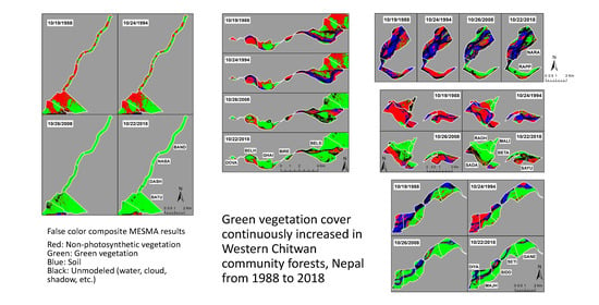
3.1. MESMA Results
3.2. Normalized Difference Fraction Index
4. Discussion
5. Conclusions
Author Contributions
Funding
Acknowledgments
Conflicts of Interest
References
- Gilmour, D. Forty Years of Community-Based Forestry: A Review of Its Extent and Effectiveness; FAO: Rome, Italy, 2016. [Google Scholar]
- Sikor, T.; Gritten, D.; Atkinson, J.; Huy, B.; Ram Dahal, G.; Duangsathaporn, K.; Hurahura, F.; Phanvilay, K.; Maryudi, A.; Pulhin, J.; et al. Community Forestry in Asia and the Pacific: Pathway to Inclusive Development; RECOFTC: Bangkok, Thailand, 2013. [Google Scholar]
- Coppin, P.R.; Bauer, M.E. Digital change detection in forest ecosystems with remote sensing imagery. Remote Sens. Rev. 1996, 13, 207–234. [Google Scholar] [CrossRef]
- Potapov, P.; Yaroshenko, A.; Turubanova, S.; Dubinin, M.; Laestadius, L.; Thies, C.; Aksenov, D.; Egorov, A.; Yesipova, Y.; Glushkov, I.; et al. Mapping the world’s intact forest landscapes by remote sensing. Ecol. Soc. 2008, 13, 51. [Google Scholar] [CrossRef]
- Kim, D.-H.; Sexton, J.O.; Noojipady, P.; Huang, C.; Anand, A.; Channan, S.; Feng, M.; Townshend, J.R. Global Landsat-Based forest-cover change from 1990 to 2000. Remote Sens. Environ. 2014, 155, 178–193. [Google Scholar] [CrossRef]
- Rouse, J.W.; Hass, R.H.; Schell, J.A.; Deering, D.W. Monitoring vegetation systems in the Great Plains with ERTS. In Proceedings of the Third ERTS Symposium 1973, Washington, DC, USA, 10–14 December 1973; Freden, S.C., Mercanti, E.P., Becker, M.A., Eds.; pp. 309–317. [Google Scholar]
- Huete, A.R. A Soil-Adjusted Vegetation Index (SAVI). Remote Sens. Environ. 1988, 25, 295–309. [Google Scholar] [CrossRef]
- Qi, J.; Chehbouni, A.; Huete, A.R.; Kerr, Y.H.; Sorooshian, S. A modified soil adjusted vegetation index. Remote Sens. Environ. 1994, 48, 119. [Google Scholar] [CrossRef]
- Liu, H.; Huete, A. A feedback based modification of the NDVI to minimize canopy background and atmospheric noise. IEEE Trans. Geosci. Remote Sens. 1995, 33, 457–465. [Google Scholar] [CrossRef]
- Saleska, S.R.; Didan, K.; Huete, A.R.; da Rocha, H.R. Amazon forests green-up during 2005 drought. Science 2007, 318, 612. [Google Scholar] [CrossRef]
- Samanta, A.; Ganguly, S.; Hashimoto, H.; Devadiga, S.; Vermote, E.; Knyazikhin, Y.; Nemani, R.R.; Myneni, R.B. Amazon forests did not green-up during the 2005 drought. Geophys. Res. Lett. 2010, 37, L05401. [Google Scholar] [CrossRef]
- Zhang, G.; Zhang, Y.; Dong, J.; Xiao, X. Green-up dates in the Tibetan Plateau have continuously advanced from 1982 to 2011. PNAS 2013, 110, 4309–4314. [Google Scholar] [CrossRef]
- Shen, M.; Sun, Z.; Wang, S.; Zhang, G.; Kong, W.; Chen, A.; Piao, S. No evidence of continuously advanced green-up dates in the Tibetan Plateau over the last decade. PNAS 2013, 110, E2329. [Google Scholar] [CrossRef]
- Adams, J.B.; Sabol, D.E.; Kapos, V.; Filho, R.A.; Roberts, D.A.; Smith, M.O.; Gillespie, A.R. Classification of multispectral images based on fractions of endmembers: Application to land-cover change in the Brazilian Amazon. Remote Sens. Environ. 1995, 52, 137–154. [Google Scholar] [CrossRef]
- Roberts, D.; Gardner, M.; Church, R.; Ustin, S.; Scheer, G.; Green, R. Mapping chaparral in the Santa Monica Mountains using multiple endmember spectral mixture models. Remote Sens. Environ. 1998, 65, 267–279. [Google Scholar] [CrossRef]
- Souza, C.M., Jr.; Roberts, D.A.; Cochrane, M.A. Combining spectral and spatial information to map canopy damage from selective logging and forest fires. Remote Sens. Environ. 2005, 98, 329–343. [Google Scholar] [CrossRef]
- Souza, C.M., Jr.; Siqueira, J.V.; Sales, M.H.; Fonseca, A.V.; RIberio, J.G.; Numata, I.; Cocharane, M.A.; Barber, C.P.; Roberts, D.A.; Barlow, J. Ten-year Landsat classification of deforestation and forest degradation in the Brazilian Amazon. Remote Sens. 2013, 5, 5493–5513. [Google Scholar] [CrossRef]
- Nagendra, H. Tenure and forest conditions: Community forestry in the Nepal Terai. Environ. Conserv. 2002, 29, 530–539. [Google Scholar] [CrossRef]
- Murphy, S.T.; Subedi, N.; Jnawali, S.R.; Lamichhane, B.R.; Upadhyay, G.P.; Kock, R.; Amin, R. Invasive mikania in Chitwan National Park, Nepal: The threat to the greater one-horned rhinoceros Rhinoceros unicornis and factors driving the invasion. Oryx 2013, 47, 361–368. [Google Scholar] [CrossRef]
- Ministry of Forest and Soil Conservation (MFSC). Persistence and Change: Review of 30 Years of Community Forestry in Nepal; Government of Nepal: Kathmandu, Nepal, 2013.
- Acharya, K.P. Twenty-four years of community forestry in Nepal. Int. For. Rev. 2014, 4, 149–156. [Google Scholar] [CrossRef]
- Mbaabu, P.R.; Hussin, Y.A.; Weir, M.; Gilani, H. Quantification of carbon stock to understand two different forest management regimes in Kayar Khola watershed, Chitwan, Nepal. J. Indian Soc. Remote Sens. 2014, 42, 745–754. [Google Scholar] [CrossRef]
- Dhakal, R.R.; Kafle, G.; Yadava, J.N. Comparative assessment of floristic diversity in a buffer zone community forest and a community forest of Barandabhar corridor, Chitwan, Nepal. J. Hortic. For. 2011, 3, 244–250. [Google Scholar]
- United Nations Educational, Scientific and Cultural Organization (UNESCO). World Heritage List. Available online: http://whc.unesco.org/en/list/284 (accessed on 1 December 2020).
- Critical Ecosystem Partnership Fund (CEPF). Available online: http://www.cepf.net/our-work/biodiversity-hotspots/Himalaya (accessed on 1 December 2020).
- Spiteri, A.; Nepal, S. Distributing conservation incentives in the buffer zone of Chitwan National Park, Nepal. Environ. Conserv. 2008, 35, 76–86. [Google Scholar] [CrossRef]
- Feyisa, G.L.; Meilby, H.; Fensholt, R.; Proud, S.R. Automated Water Extraction Index: A new technique for surface water mapping using Landsat imagery. Remote Sens. Environ. 2014, 140, 23–35. [Google Scholar] [CrossRef]
- Dai, J.; Roberts, D.A.; Stow, D.A.; An, L.; Hall, S.J.; Yabiku, S.T.; Kyriakidis, P.C. Mapping understory invasive plant species with field and remotely sensed data in Chitwan, Nepal. Remote Sens. Environ. 2020, 250, 112037. [Google Scholar] [CrossRef]
- Carter, N.H.; Shrestha, B.K.; Karki, J.B.; Pradhan, N.M.B.; Liu, J. Coexistence between wildlife and humans at fine spatial scales. PNAS 2012, 109, 15360–15365. [Google Scholar] [CrossRef] [PubMed]
- Niraula, R.R.; Gilani, H.; Pokharel, B.K.; Qamer, F.M. Measuring impacts of community forestry program through repeat photography and satellite remote sensing in the Dolakha district of Nepal. J. Environ. Manag. 2013, 126, 20–29. [Google Scholar] [CrossRef] [PubMed]
- Tripathi, S.; Subedi, R.; Adhikari, H. Forest Cover Change Pattern after the Intervention of Community Forestry Management System in the Mid-Hill of Nepal: A Case Study. Remote Sens. 2020, 12, 2756. [Google Scholar] [CrossRef]
- Poffenberger, M. People in the forest: Community forestry experiences from Southeast Asia. Int. J. Environ. Sustain. Dev. 2006, 5, 57–69. [Google Scholar] [CrossRef]
- Newton, P.; Schaap, B.; Fournier, M.; Cornwall, M.; Rosenbach, D.W.; DeBoer, J.; Whittemore, J.; Stock, R.; Yoders, M.; Brodnig, G.; et al. Community forest management and REDD+. For. Policy Econ. 2015, 56, 27–37. [Google Scholar] [CrossRef]


| Group | Forest Name | Code | Forest Type | Area (km2) |
|---|---|---|---|---|
| East Sal | Bandevi | BAND | Sal Forest | 1.62 |
| Nabajoty | NABA | 0.42 | ||
| Dashinkali | DASH | 1.05 | ||
| Batuliphokhari | BATU | 4.57 | ||
| South Central Rapti | Belshar | BELS | Riverine Mixed | 6.40 |
| Birendranagar | BIRE | 0.40 | ||
| Ghailaghari | GHAI | 1.82 | ||
| Belhatta | BELH | 1.21 | ||
| Dovan | DOVA | 0.23 | ||
| South West Rapti | Sayukta Rapti Doon | SAYU | Riverine Mixed | 1.36 |
| Betarihariyali | BETA | 0.87 | ||
| Malika | MALI | 0.11 | ||
| Radhakrishna | RADH | 0.82 | ||
| Sadabahar | SADA | 2.10 | ||
| Far West | Rapptiniyantran | RAPP | Riverine Mixed | 2.06 |
| Narayani Niyantran | NARA | 5.01 | ||
| North Narayani | Diyalo | DIYA | Riverine Mixed | 1.66 |
| Majhuwa | MAJH | 1.86 | ||
| Siddhi Ganesh | SIDD | 1.35 | ||
| Seti Debi | SETI | 1.51 | ||
| Ganeswor | GANE | 2.27 |
| Year | Date | Julian | Sensor | Year | Date | Julian | Sensor |
|---|---|---|---|---|---|---|---|
| 1988 | 10/19 | 293 | TM | 2005 | 11/19 | 323 | TM |
| 1989 | 11/07 | 311 | TM | 2006 | 10/05 | 278 | TM |
| 1991 | 11/13 | 317 | TM | 2008 | 10/26 | 300 | TM |
| 1992 | 11/15 | 320 | TM | 2009 | 10/29 | 302 | TM |
| 1993 | 10/17 | 290 | TM | 2011 | 10/19 | 292 | TM |
| 1994 | 10/20 | 293 | TM | 2013 | 11/19 | 323 | OLI |
| 1995 | 11/08 | 312 | TM | 2014 | 10/27 | 300 | OLI |
| 1996 | 11/10 | 315 | TM | 2015 | 10/14 | 287 | OLI |
| 2000 | 09/26 | 270 | ETM+ | 2016 | 11/01 | 306 | OLI |
| 2001 | 10/31 | 304 | ETM+ | 2017 | 10/19 | 292 | OLI |
| 2003 | 11/14 | 318 | TM | 2018 | 10/22 | 295 | OLI |
| 2004 | 10/15 | 289 | TM |
| Bands | TM/ETM+ | OLI |
|---|---|---|
| Green | Band 2 (520–600 nm) | Band 3 (525–600 nm) |
| NIR | Band 4 (760–900 nm) | Band 5 (845–885 nm) |
| SWIR1 | Band 5 (1550–1750 nm) | Band 6 (1560–1660 nm) |
| SWIR2 | Band 7 (2080–2350 nm) | Band 7 (2100–2300 nm) |
| Periods | Years Selected |
|---|---|
| I (Pre 1993) | 1988, 1989, 1991, 1992, 1993 |
| II (1994–1999) | 1994, 1995, 1996 |
| III (2000s) | 2003, 2004, 2005, 2008, 2009 |
| IV (2010s) | 2013, 2014, 2016, 2018 |
| Group | Forest | GV |
|---|---|---|
| East Sal | BAND | 0.79 |
| NABA | 0.70 | |
| DASH | 0.65 | |
| BATU | 0.72 | |
| South Central Rapti | BELS | 0.46 |
| BIRE | 0.33 | |
| GHAI | 0.56 | |
| BELH | 0.29 | |
| DOVA | 0.43 | |
| South West Rapti | SAYU | 0.20 |
| BETA | 0.45 | |
| MALI | 0.74 | |
| RADH | 0.57 | |
| SADA | 0.30 | |
| Far West | RAPP | 0.34 |
| NARA | 0.21 | |
| North Narayani | DIYA | 0.39 |
| MAJH | 0.57 | |
| SIDD | 0.61 | |
| SETI | 0.60 | |
| GANE | 0.68 |
| Group (4) | Forest | I vs. II | II vs. III | III vs. IV | I vs. III | II vs. IV | I vs. IV | I vs. II~IV |
|---|---|---|---|---|---|---|---|---|
| East Sal | BAND | 3.77 × 10⁻² | 4.22 × 10⁻³ | 1.07 × 10⁻³ | 3.19 × 10⁻³ | |||
| NABA | 1.77 × 10⁻² | 3.17 × 10⁻³ | 2.20 × 10⁻² | |||||
| DASH | 4.19 × 10⁻² | 4.41 × 10⁻³ | 2.26 × 10⁻³ | 2.80 × 10⁻² | ||||
| BATU | 3.08 × 10⁻² | 1.07 × 10⁻³ | 6.47 × 10⁻⁵ | 4.98 × 10⁻⁴ | ||||
| South Central Rapti | BELS | 5.50 × 10⁻³ | 4.70 × 10⁻² | 3.89 × 10⁻⁶ | 3.86 × 10⁻⁶ | 1.83 × 10⁻³ | ||
| BIRE | 4.83 × 10⁻² | 5.14 × 10⁻³ | 7.51 × 10⁻³ | 6.75 × 10⁻³ | ||||
| GHAI | 4.02 × 10⁻² | 4.18 × 10⁻⁴ | 4.79 × 10⁻⁵ | 6.01 × 10⁻³ | ||||
| BELH | 7.12 × 10⁻³ | 1.05 × 10⁻² | 1.22 × 10⁻⁵ | 5.17 × 10⁻⁶ | 1.19 × 10⁻³ | |||
| DOVA | 8.18 × 10⁻⁵ | 1.35 × 10⁻² | 6.28 × 10⁻³ | 7.45 × 10⁻⁶ | 3.30 × 10⁻⁷ | 1.11 × 10⁻⁵ | ||
| South West Rapti | SAYU | 1.18 × 10⁻³ | 7.32 × 10⁻⁴ | 7.58 × 10⁻⁷ | 4.65 × 10⁻³ | |||
| BETA | 1.70 × 10⁻² | 4.37 × 10⁻² | 3.99 × 10⁻³ | 2.92 × 10⁻³ | 5.64 × 10⁻⁷ | 6.65 × 10⁻⁵ | ||
| MALI | 3.91 × 10⁻² | 1.18 × 10⁻² | 1.73 × 10⁻³ | 1.46 × 10⁻³ | ||||
| RADH | 1.97 × 10⁻² | 1.38 × 10⁻² | 4.48 × 10⁻² | 7.38 × 10⁻³ | 1.24 × 10⁻³ | 2.86 × 10⁻⁶ | 2.86 × 10⁻⁶ | |
| SADA | 4.45 × 10⁻² | 5.09 × 10⁻³ | 3.84 × 10⁻² | 3.77 × 10⁻⁸ | 8.05 × 10⁻¹⁰ | 1.63 × 10⁻³ | ||
| Far West | RAPP | 1.69 × 10⁻² | 2.77 × 10⁻² | 1.53 × 10⁻² | 9.23 × 10⁻⁷ | 8.05 × 10⁻⁷ | 6.22 × 10⁻⁴ | |
| NARA | 4.42 × 10⁻² | 6.99 × 10⁻⁴ | 4.03 × 10⁻⁴ | 7.41 × 10⁻³ | ||||
| North Narayani | DIYA | 1.24 × 10⁻² | 1.35 × 10⁻² | 2.37 × 10⁻⁵ | 8.10 × 10⁻⁶ | 5.44 × 10⁻⁴ | ||
| MAJH | 1.91 × 10⁻² | 1.09 × 10⁻⁴ | 1.16 × 10⁻² | |||||
| SIDD | 2.91 × 10⁻² | |||||||
| SETI | 3.78 × 10⁻² | 2.11 × 10⁻⁴ | 1.73 × 10⁻⁴ | 1.72 × 10⁻² | ||||
| GANE | 3.70 × 10⁻² | 2.53 × 10⁻⁴ | 1.60 × 10⁻⁴ | 7.50 × 10⁻³ |
| Group | Forest | NDFI |
|---|---|---|
| East Sal | BAND | 0.67 |
| NABA | 0.52 | |
| DASH | 0.44 | |
| BATU | 0.56 | |
| South Central Rapti | BELS | 0.11 |
| BIRE | −0.09 | |
| GHAI | 0.32 | |
| BELH | −0.21 | |
| DOVA | 0.06 | |
| South West Rapti | SAYU | −0.43 |
| BETA | 0.05 | |
| MALI | 0.59 | |
| RADH | 0.27 | |
| SADA | −0.21 | |
| Far West | RAPP | −0.12 |
| NARA | −0.54 | |
| North Narayani | DIYA | −0.13 |
| MAJH | 0.19 | |
| SIDD | 0.29 | |
| SETI | 0.25 | |
| GANE | 0.43 |
| Group | Forest | I vs. II | II vs. III | III vs. IV | I vs. III | II vs. IV | I vs. IV | I vs. II~IV |
|---|---|---|---|---|---|---|---|---|
| East Sal | BAND | 4.78 × 10⁻⁴ | 1.16 × 10⁻³ | 3.50 × 10⁻³ | 1.22 × 10⁻³ | 1.54 × 10⁻³ | ||
| NABA | 1.18 × 10⁻² | 5.15 × 10⁻³ | 1.66 × 10⁻² | 3.60 × 10⁻³ | 1.17 × 10⁻² | |||
| DASH | 1.20 × 10⁻³ | 4.81 × 10⁻² | 3.29 × 10⁻³ | 4.63 × 10⁻³ | 2.61 × 10⁻³ | 1.10 × 10⁻² | ||
| BATU | 3.48 × 10⁻⁵ | 6.43 × 10⁻⁶ | 1.38 × 10⁻³ | 6.64 × 10⁻⁵ | 2.13 × 10⁻⁵ | |||
| South Central Rapti | BELS | 7.75 × 10⁻³ | 5.53 × 10⁻³ | 5.07 × 10⁻³ | 9.64 × 10⁻⁶ | 1.34 × 10⁻⁶ | 5.44 × 10⁻⁴ | |
| BIRE | 6.86 × 10⁻³ | 2.14 × 10⁻⁶ | 9.27 × 10⁻⁸ | 1.46 × 10⁻² | ||||
| GHAI | 2.00 × 10⁻² | 2.98 × 10⁻² | 9.71 × 10⁻³ | 4.22 × 10⁻⁴ | 2.39 × 10⁻⁵ | 4.50 × 10⁻⁴ | ||
| BELH | 9.17 × 10⁻³ | 7.68 × 10⁻³ | 1.11 × 10⁻³ | 8.87 × 10⁻⁴ | 1.70 × 10⁻³ | |||
| DOVA | 1.22 × 10⁻⁴ | 5.23 × 10⁻³ | 5.07 × 10⁻³ | 4.65 × 10⁻⁴ | 8.29 × 10⁻⁷ | 7.73 × 10⁻⁹ | 1.11 × 10⁻⁵ | |
| South West Rapti | SAYU | 2.12 × 10⁻⁴ | 4.22 × 10⁻⁴ | 3.26 × 10⁻⁴ | 6.17 × 10⁻³ | |||
| BETA | 3.21 × 10⁻³ | 2.30 × 10⁻² | 9.69 × 10⁻⁴ | 1.77 × 10⁻³ | 3.66 × 10⁻⁶ | 4.56 × 10⁻⁵ | ||
| MALI | 2.17 × 10⁻³ | 2.12 × 10⁻³ | 1.73 × 10⁻³ | |||||
| RADH | 2.50 × 10⁻² | 1.56 × 10⁻⁵ | 3.28 × 10⁻⁶ | 1.17 × 10⁻³ | 2.83 × 10⁻⁶ | 8.13 × 10⁻⁶ | ||
| SADA | 1.78 × 10⁻² | 2.46 × 10⁻³ | 1.67 × 10⁻² | 1.89 × 10⁻⁶ | 1.82 × 10⁻⁷ | 1.38 × 10⁻³ | ||
| Far West | RAPP | 6.39 × 10⁻³ | 2.84 × 10⁻² | 6.34 × 10⁻³ | 3.00 × 10⁻⁷ | 3.16 × 10⁻⁷ | 3.78 × 10⁻⁴ | |
| NARA | 3.18 × 10⁻² | 4.25 × 10⁻² | 3.25 × 10⁻⁴ | 2.29 × 10⁻⁴ | 3.86 × 10⁻³ | |||
| North Narayani | DIYA | 3.20 × 10⁻³ | 3.77 × 10⁻³ | 1.64 × 10⁻⁵ | 1.31 × 10⁻⁶ | 2.69 × 10⁻⁴ | ||
| MAJH | 2.10 × 10⁻² | 1.65 × 10⁻² | 1.44 × 10⁻² | 8.58 × 10⁻⁵ | 3.50 × 10⁻³ | |||
| SIDD | 1.57 × 10⁻² | |||||||
| SETI | 2.01 × 10⁻² | 3.98 × 10⁻⁴ | 5.97 × 10⁻⁵ | 5.01 × 10⁻³ | ||||
| GANE | 2.96 × 10⁻² | 2.22 × 10⁻² | 1.40 × 10⁻³ | 1.20 × 10⁻⁴ | 4.96 × 10⁻⁴ |
Publisher’s Note: MDPI stays neutral with regard to jurisdictional claims in published maps and institutional affiliations |
© 2020 by the authors. Licensee MDPI, Basel, Switzerland. This article is an open access article distributed under the terms and conditions of the Creative Commons Attribution (CC BY) license (http://creativecommons.org/licenses/by/4.0/).
Share and Cite
Dai, J.; Roberts, D.A.; Stow, D.A.; An, L.; Zhao, Q. Green Vegetation Cover Has Steadily Increased since Establishment of Community Forests in Western Chitwan, Nepal. Remote Sens. 2020, 12, 4071. https://doi.org/10.3390/rs12244071
Dai J, Roberts DA, Stow DA, An L, Zhao Q. Green Vegetation Cover Has Steadily Increased since Establishment of Community Forests in Western Chitwan, Nepal. Remote Sensing. 2020; 12(24):4071. https://doi.org/10.3390/rs12244071
Chicago/Turabian StyleDai, Jie, Dar A. Roberts, Douglas A. Stow, Li An, and Qunshan Zhao. 2020. "Green Vegetation Cover Has Steadily Increased since Establishment of Community Forests in Western Chitwan, Nepal" Remote Sensing 12, no. 24: 4071. https://doi.org/10.3390/rs12244071
APA StyleDai, J., Roberts, D. A., Stow, D. A., An, L., & Zhao, Q. (2020). Green Vegetation Cover Has Steadily Increased since Establishment of Community Forests in Western Chitwan, Nepal. Remote Sensing, 12(24), 4071. https://doi.org/10.3390/rs12244071