Long-Term Grass Biomass Estimation of Pastures from Satellite Data

 ,
, 
Abstract

1. Introduction
2. Study Area and Datasets
2.1. Zambia Country’s Profile
2.1.1. Zambia Strategies in Livestock Sector
2.1.2. Zambia Grazing Areas
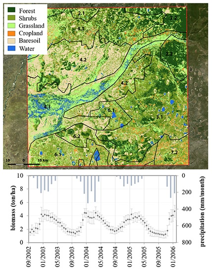
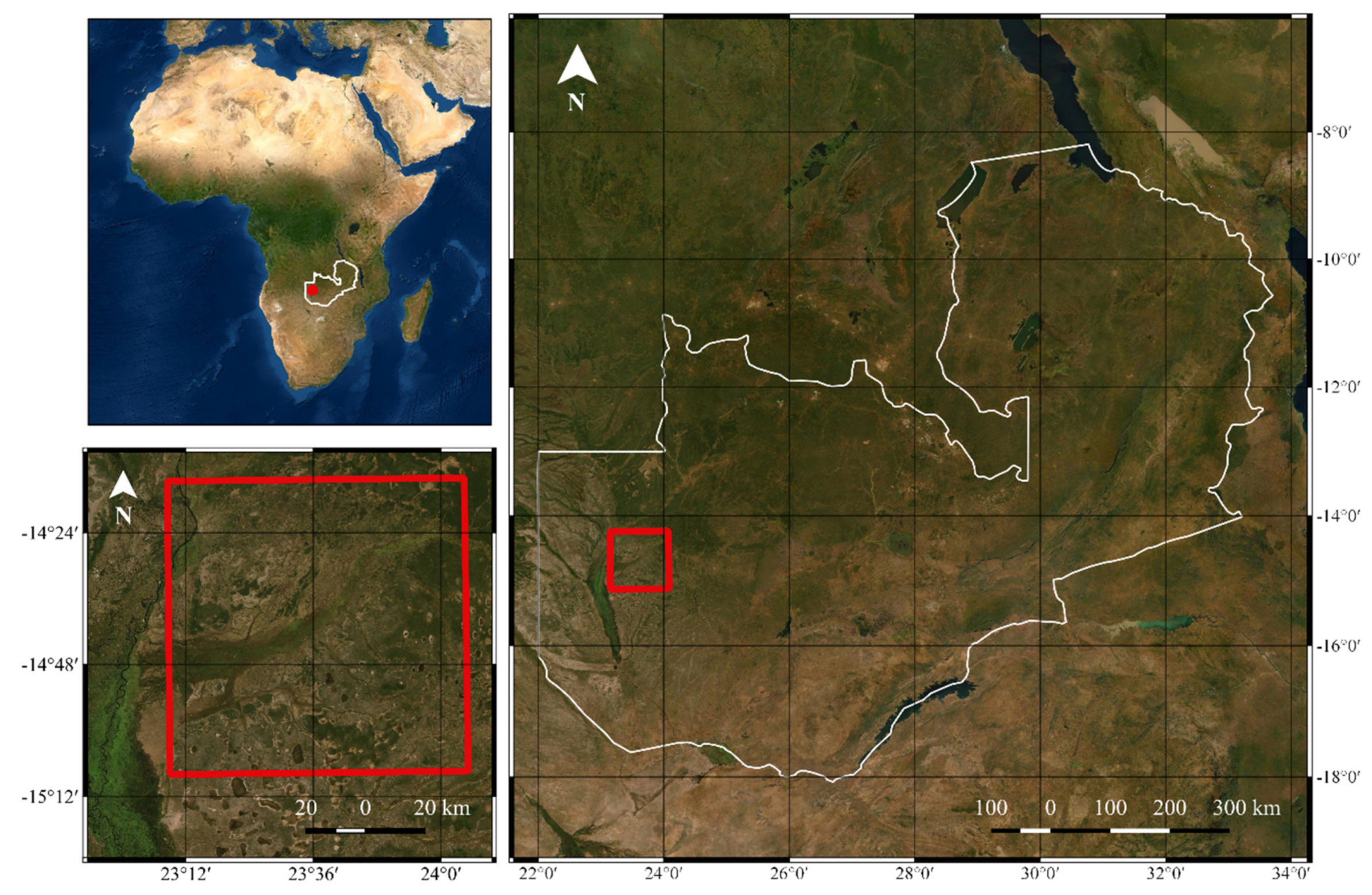
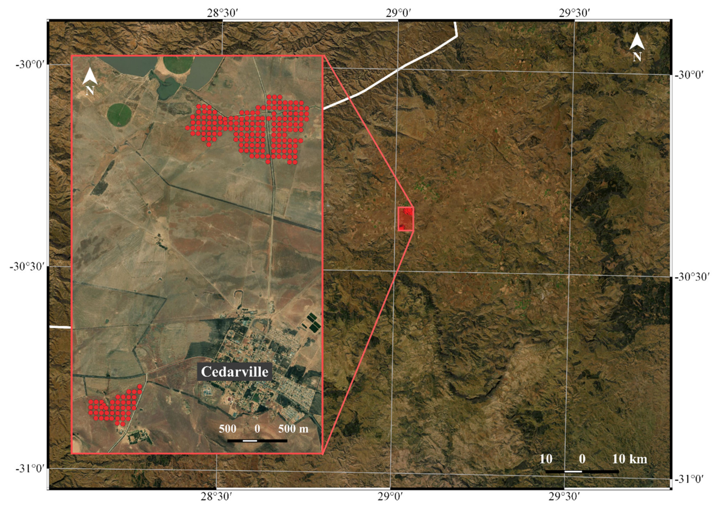
2.2. Study Area
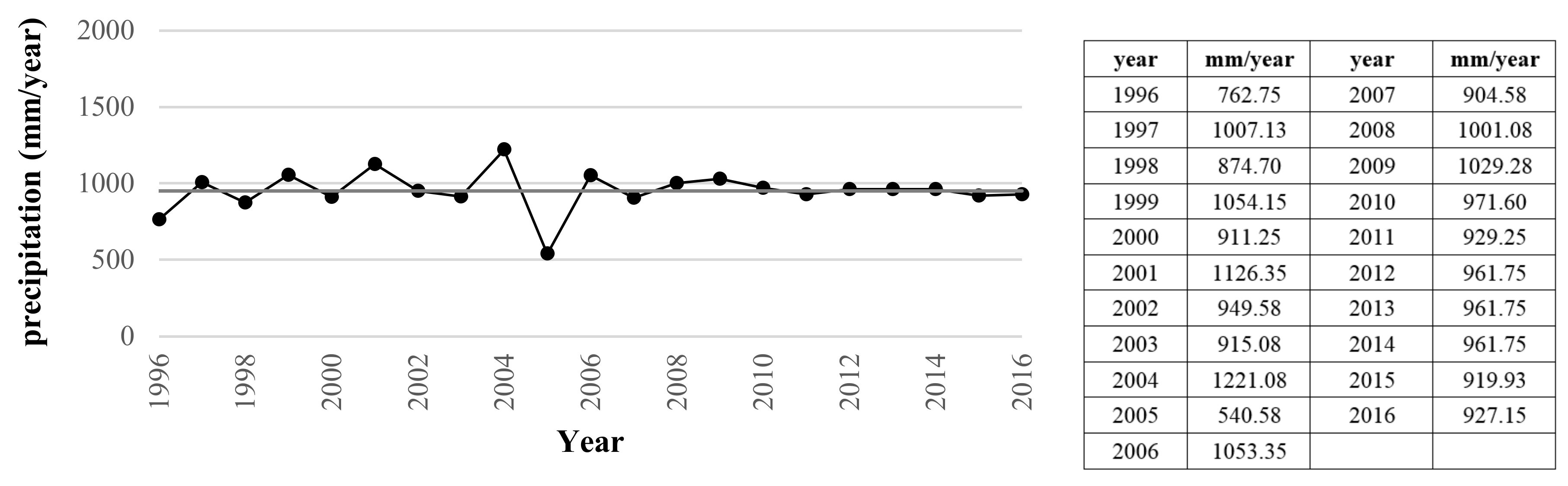
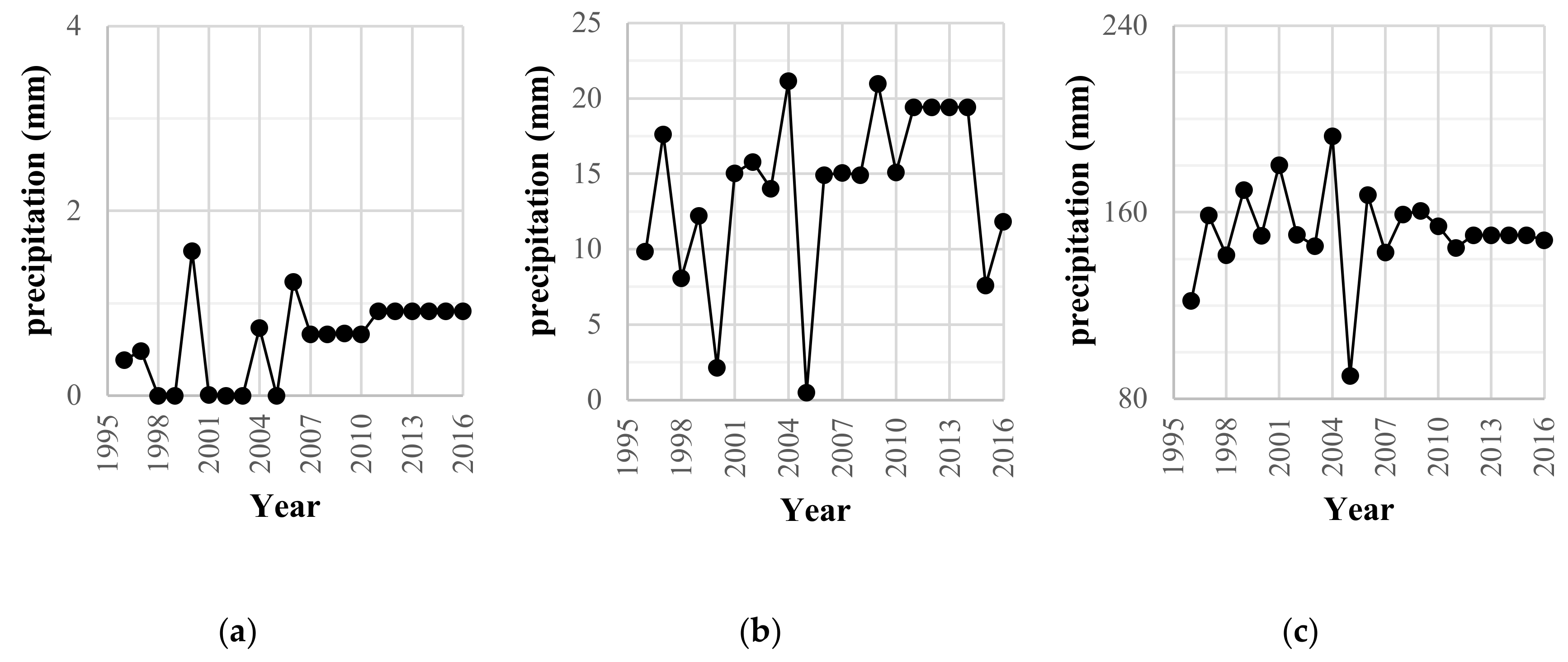
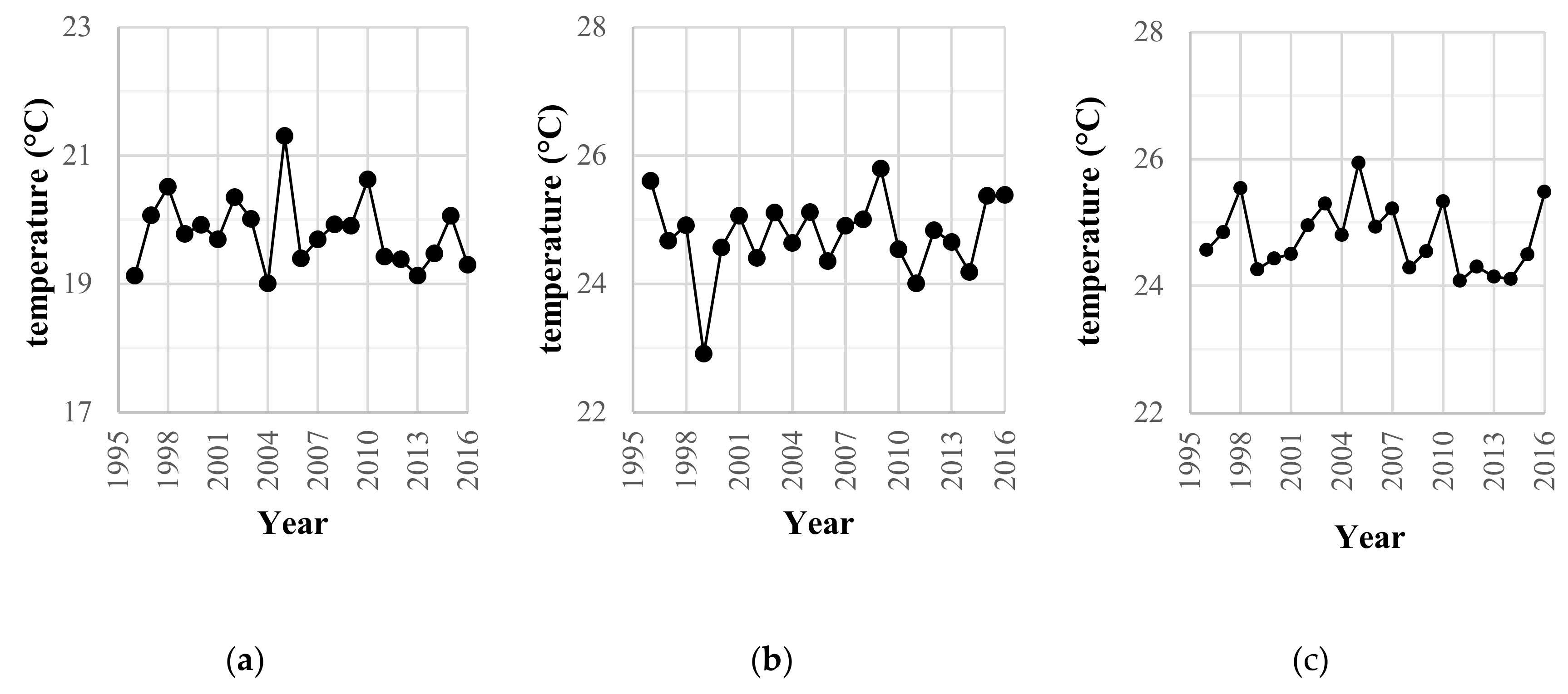
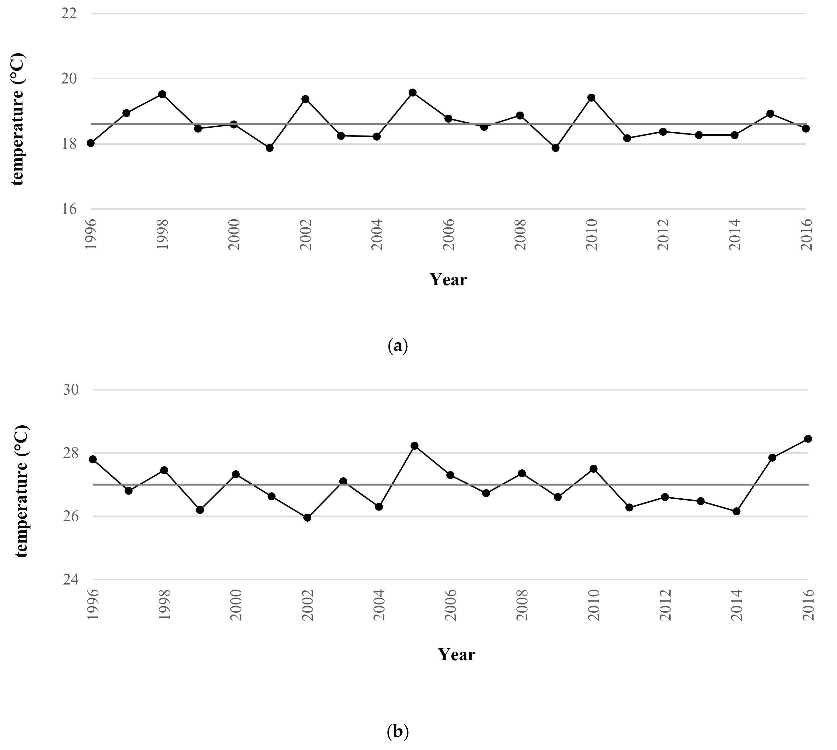
2.2.1. Climatic Data
2.2.2. Land Cover Classification Dataset
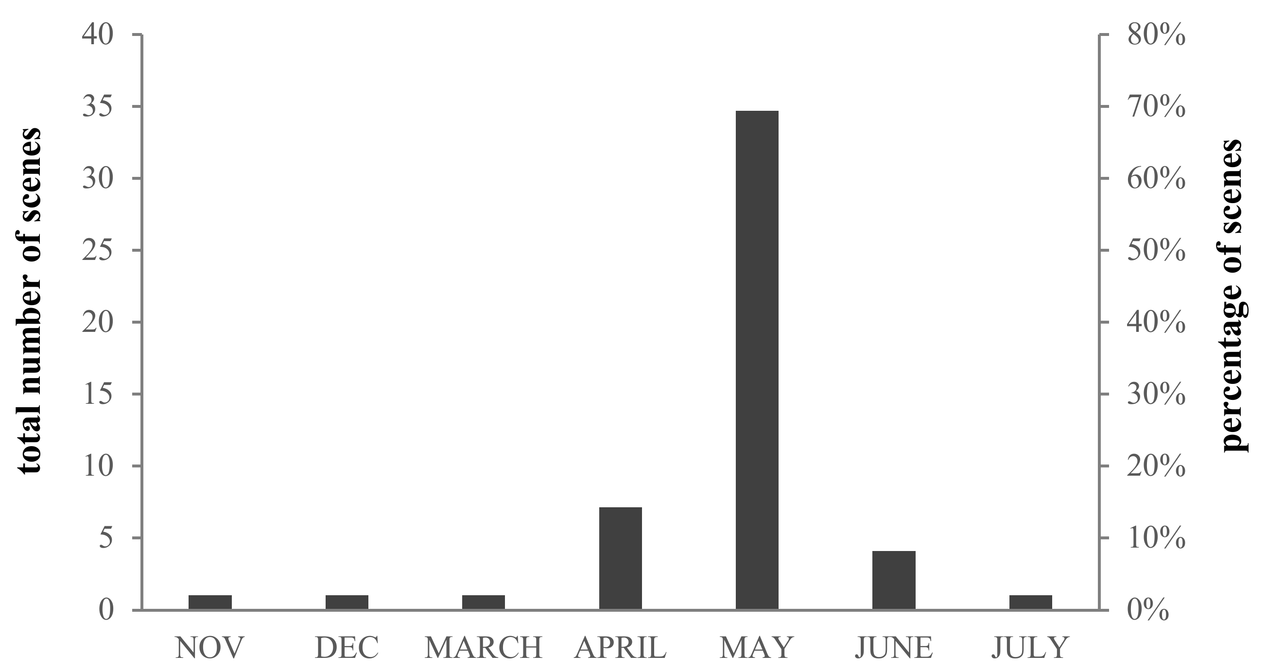
2.2.3. Growth Cycle and Biomass Dataset
3. Methodology
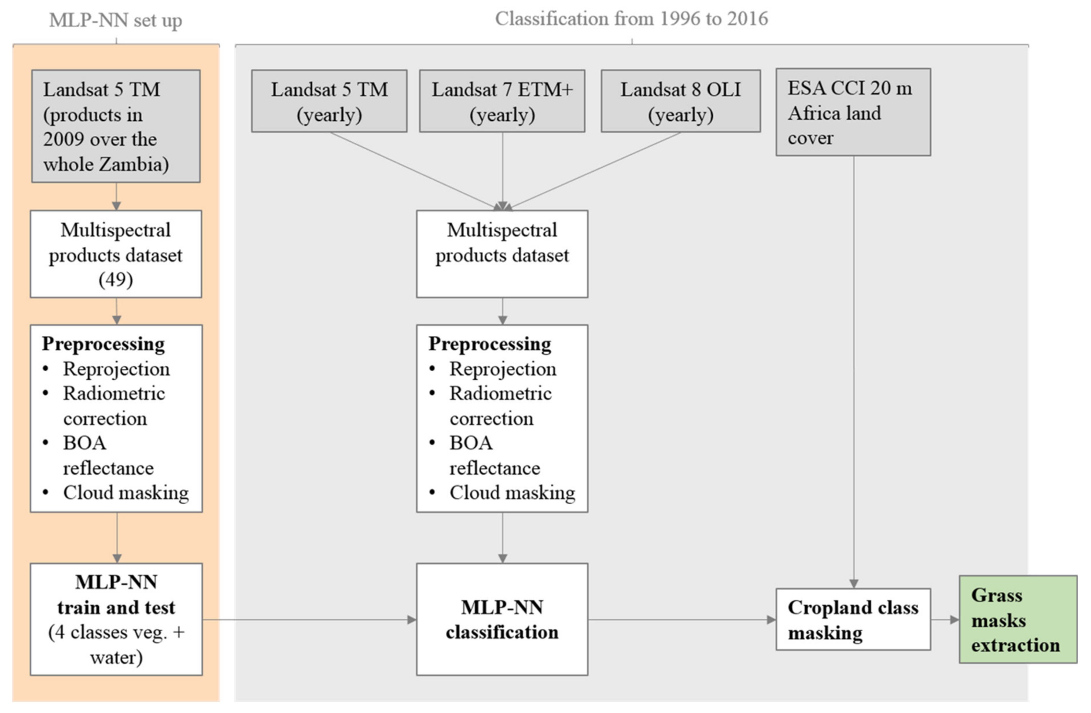
3.1. Land Cover Classification
3.1.1. Multi-Layer Perceptron Classifier
3.1.2. Grass Area Extraction
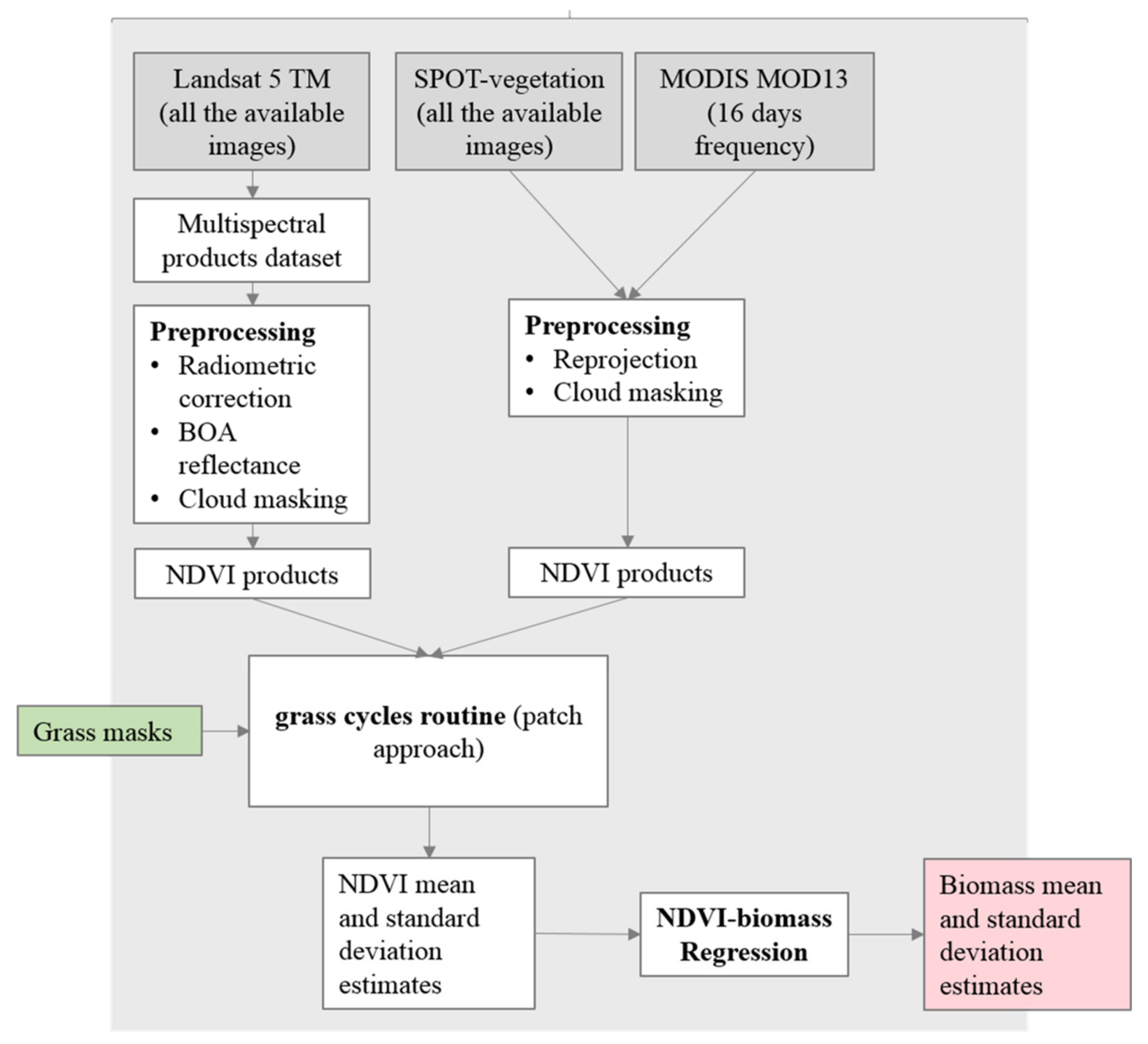
3.2. Growth Cycles and Biomass Estimation
3.2.1. Regression Model
3.2.2. Long-Term Grass Biomass Estimates
4. Results
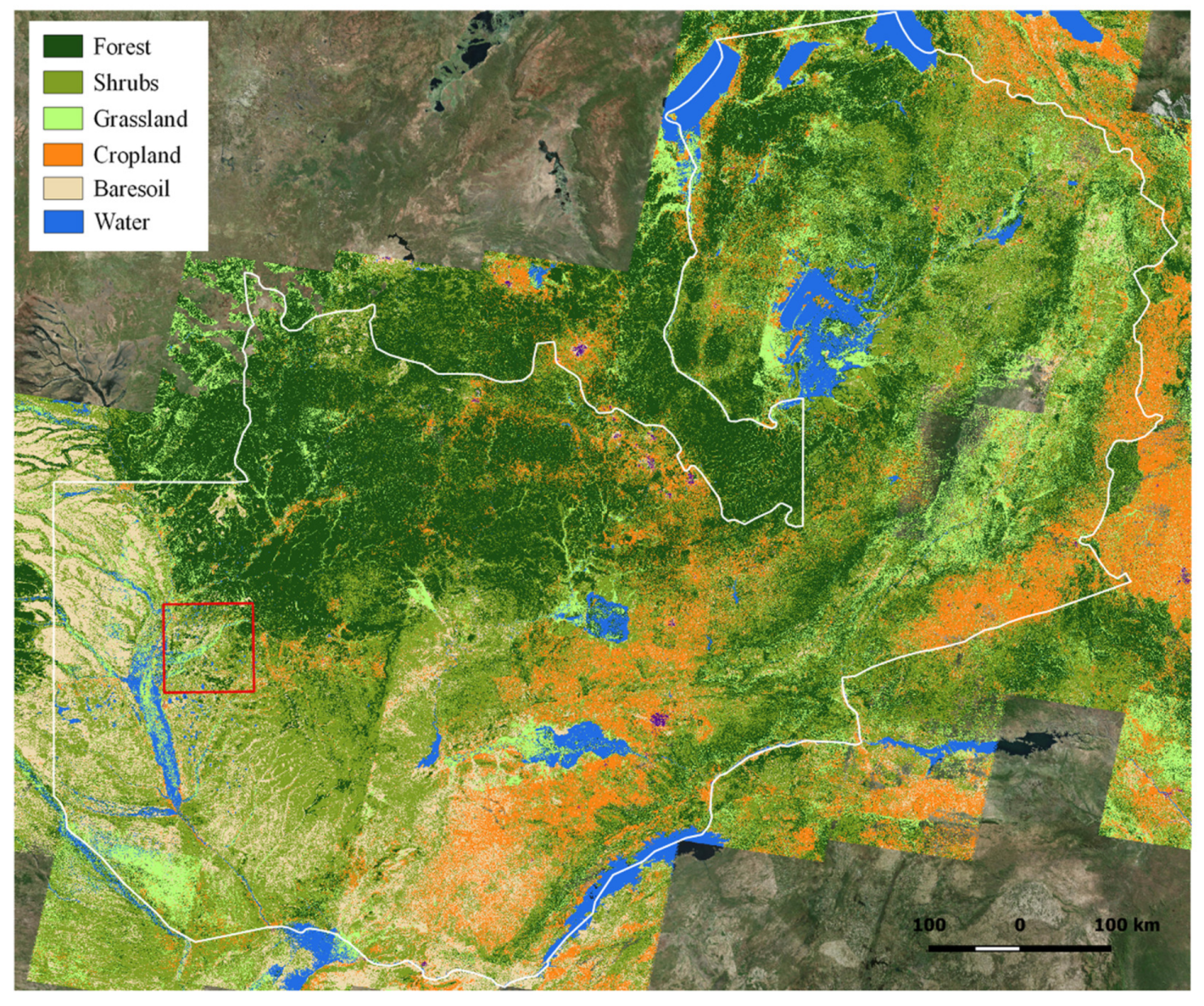
4.1. Land Cover Classification
4.2. Biomass
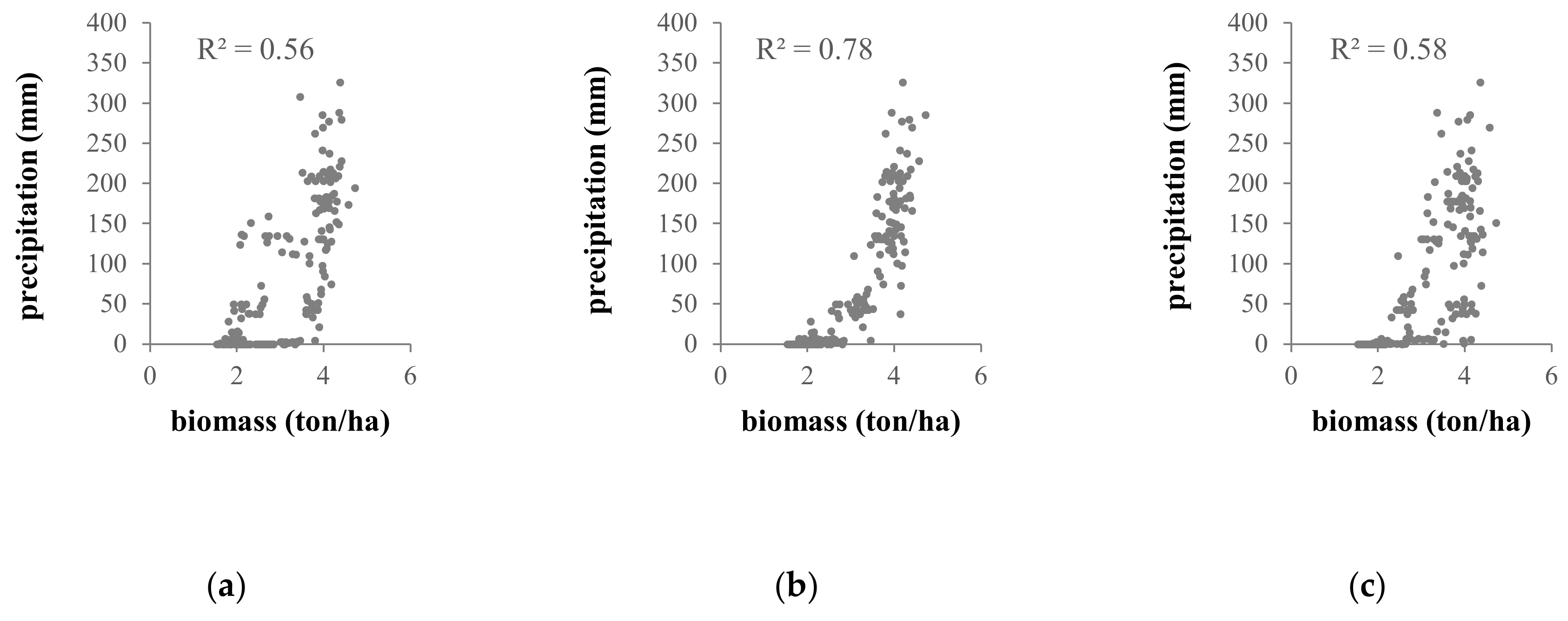
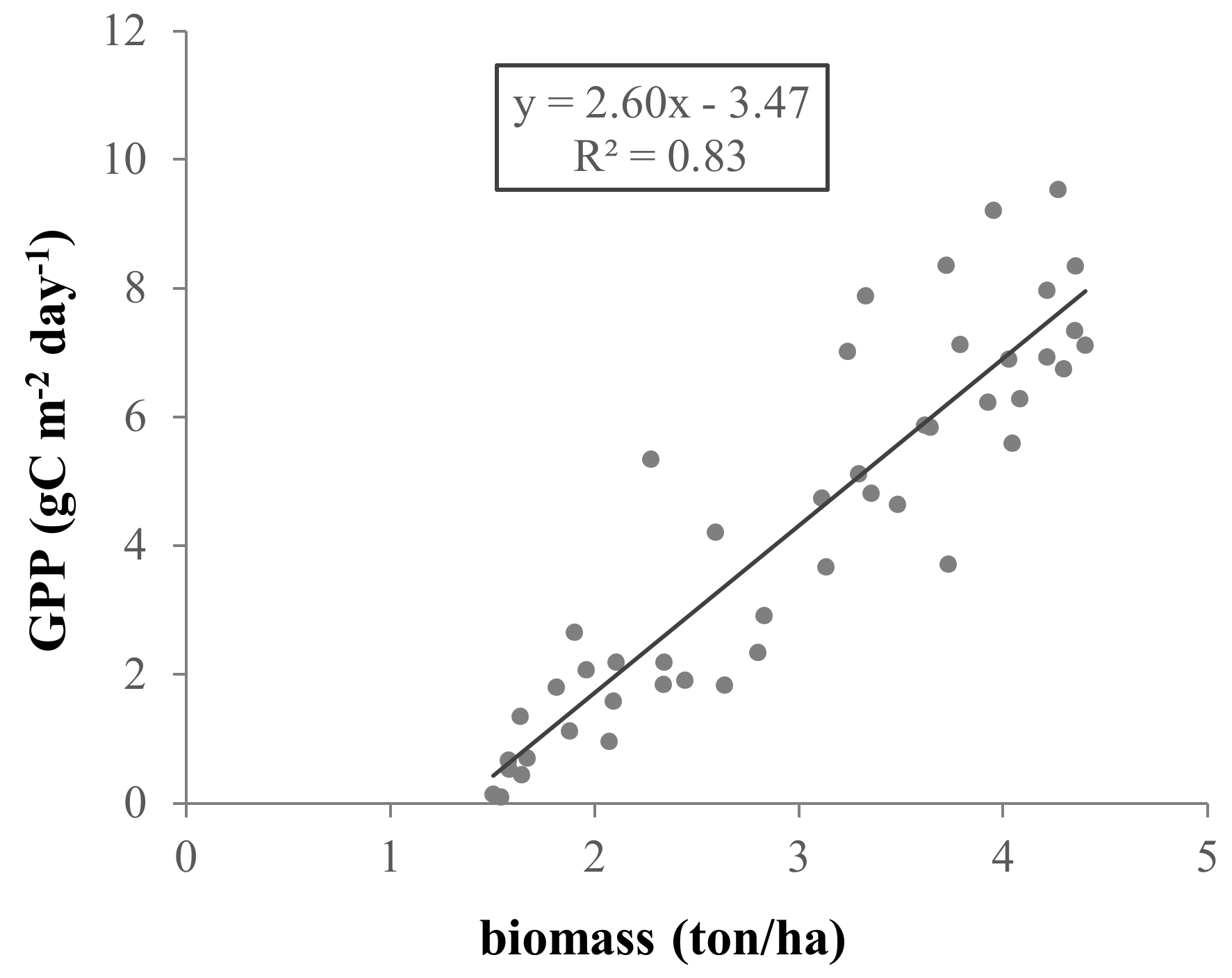
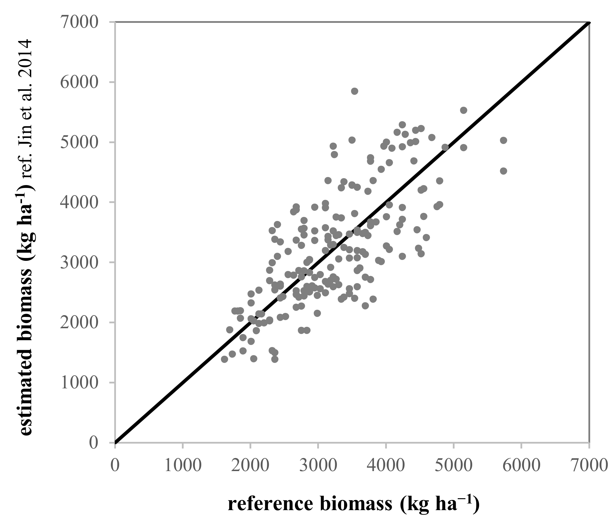
4.2.1. Regression Analysis
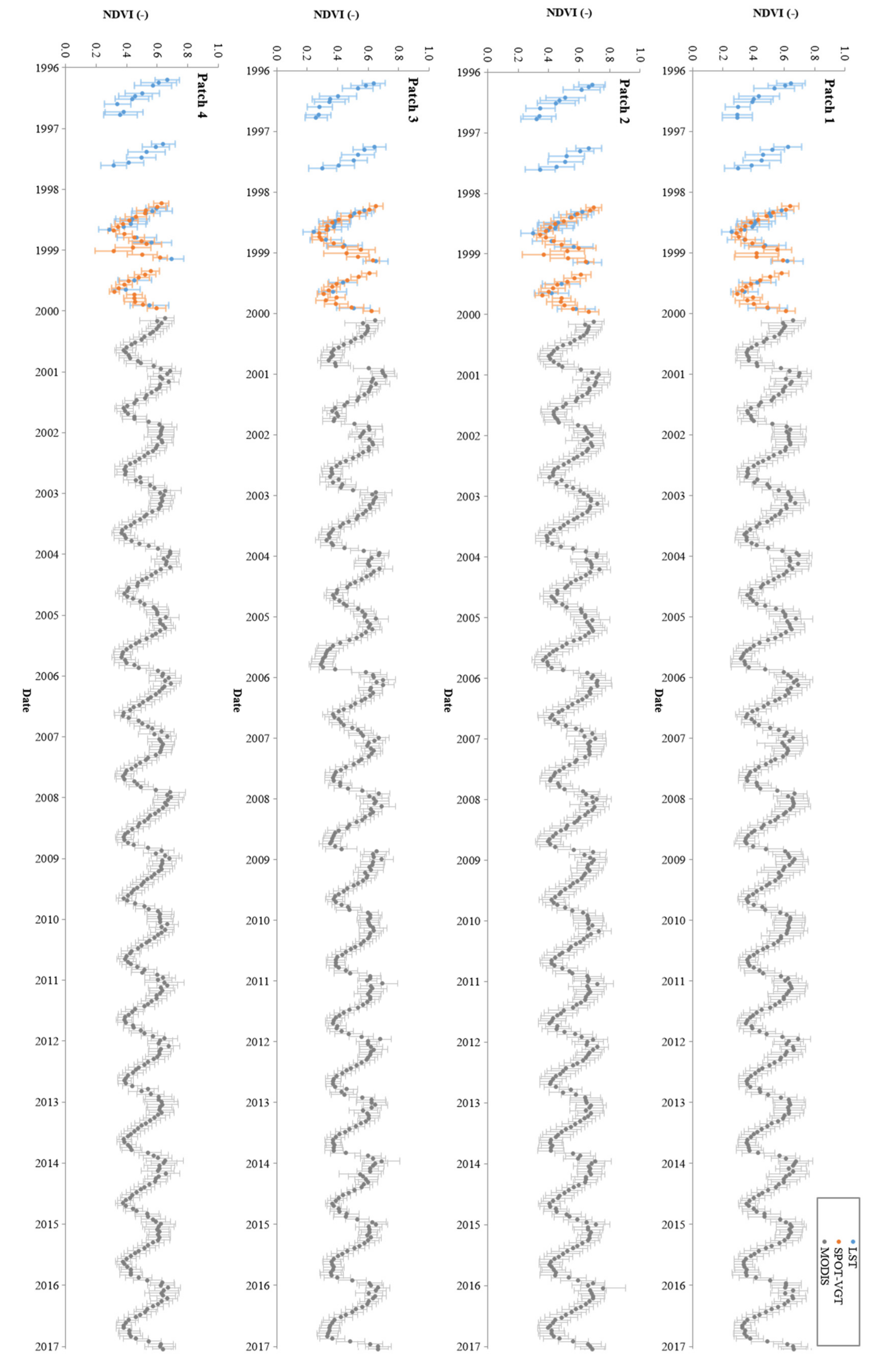
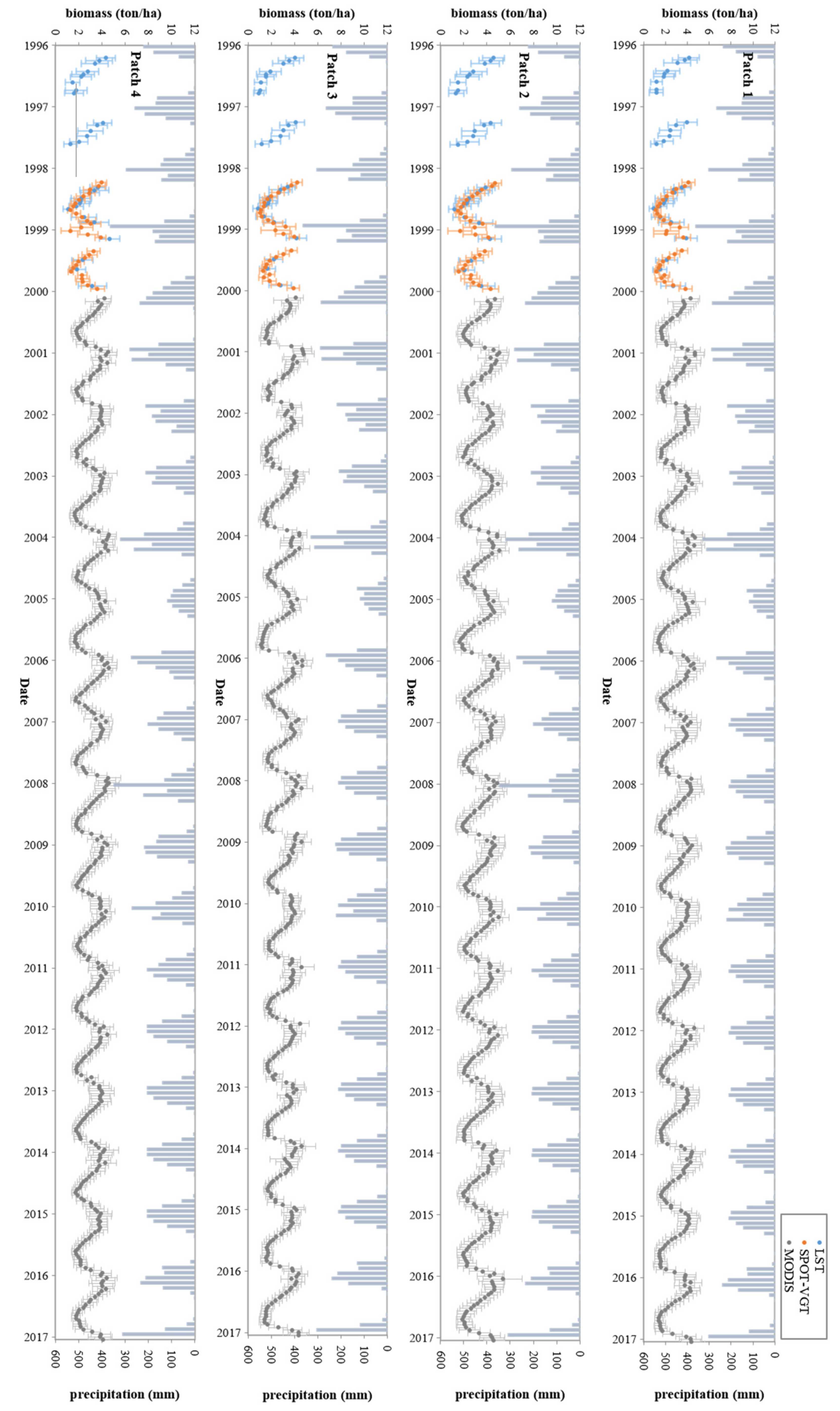
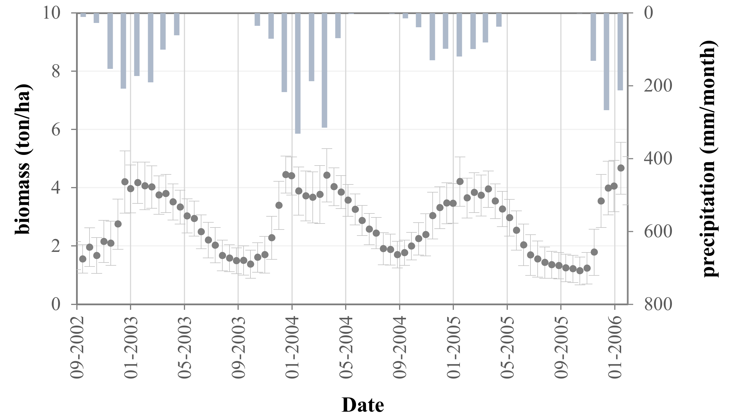
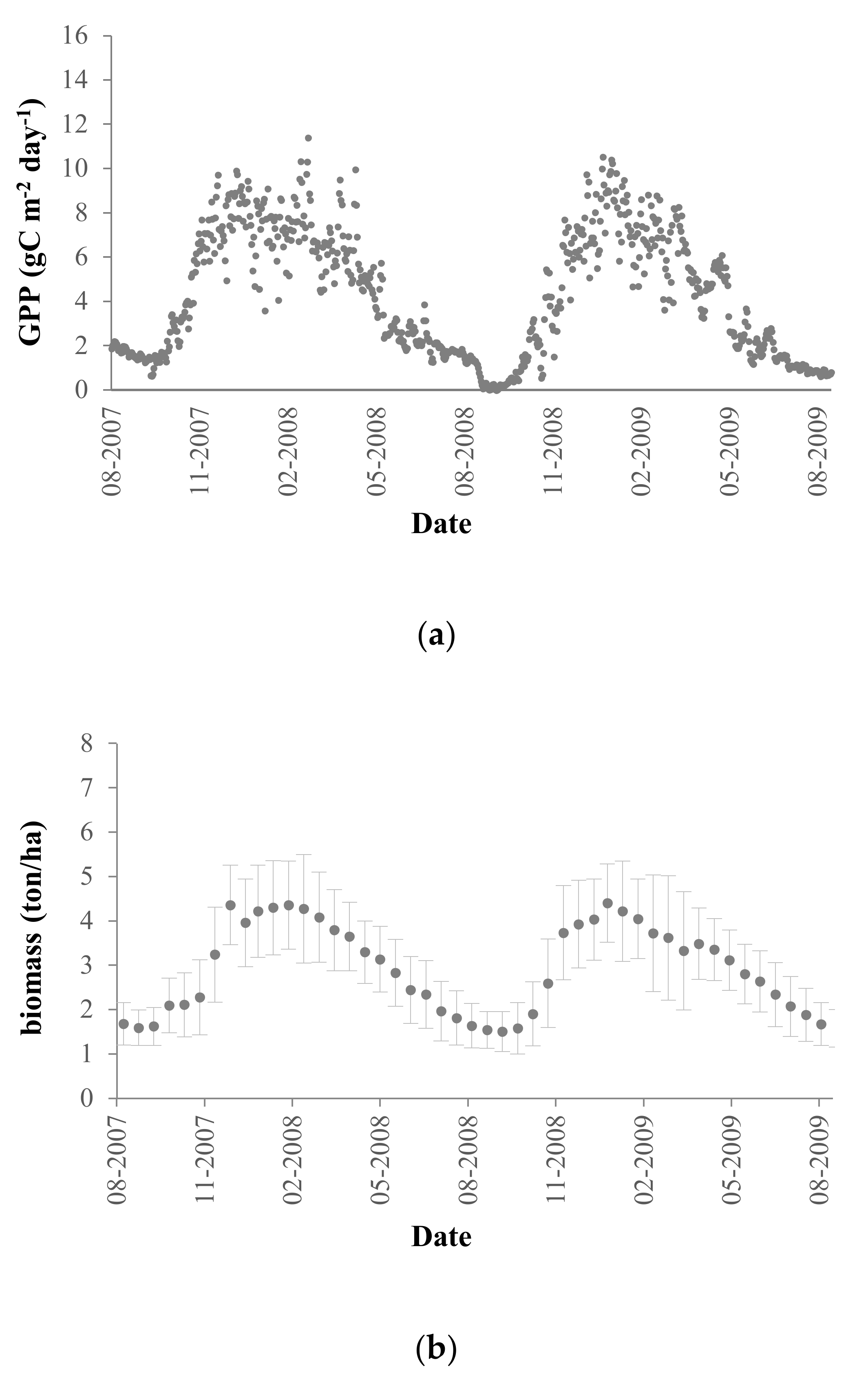
4.2.2. Growth Cycles and Biomass
5. Discussion
6. Conclusions
Author Contributions
Funding
Acknowledgments
Conflicts of Interest
References
- IPCC. Climate Change 2013: The Physical Science Basis. In Contribution of Working Group I to the Fifth Assessment Report of the Intergovernmental Panel on Climate Change; Stocker, T.F., Qin, D., Plattner, G.-K., Tignor, M., Allen, S.K., Boschung, J., Nauels, A., Xia, Y., Bex, V., Midgley, P.M., Eds.; Cambridge University Press: Cambridge, UK; New York, NY, USA, 2013; p. 1535. [Google Scholar] [CrossRef]
- Guerschman, J.; Held, A.; Donohue, R.; Renzullo, L.; Sims, N.; Kerblat, F.; Grundy, M. The GEOGLAM rangelands and pasture productivity activity: Recent progress and future directions. AGU Fall Meet. Abstr. 2015, 43, B43A–B0531. [Google Scholar]
- Gerber, P.J.; Steinfeld, H.; Henderson, B.; Mottet, A.; Opio, C.; Dijkman, J.; Falcucci, A.; Tempio, G. Tackling Climate Change through Livestock–A Global Assessment of Emissions and Mitigation Opportunities; Food and Agriculture Organization of the United Nations: Rome, Italy, 2013. [Google Scholar]
- Kuik, O.; Reynes, F.; Delobel, F.; Bernardi, M. FAO-MOSAICC: The FAO modelling system for agricultural impacts of climate change to support decision-making in adaptation. In Proceedings of the 14th GTAP Conference, Venice, Italy, 16–18 June 2011. [Google Scholar]
- Ali, I.; Greifeneder, F.; Stamenkovic, J.; Neumann, M.; Notarnicola, C. Review of machine learning approaches for biomass and soil moisture retrievals from remote sensing data. Remote Sens. 2015, 7, 16398–16421. [Google Scholar] [CrossRef]
- Pacifici, F.; Del Frate, F.; Solimini, C.; Emery, W.J. Neural networks for land cover applications. Comput. Intell. Remote. Sens. 2008, 133, 267–293. [Google Scholar]
- Dixon, B.; Candade, N. Multispectral landuse classification using neural networks and support vector machines: one or the other, or both? Int. J. Remote Sens. 2008, 29, 1185–1206. [Google Scholar] [CrossRef]
- Foody, G.M.; McCulloch, M.B.; Yates, W.B. Classification of remotely sensed data by an artificial neural network: Issues related to training data. Photogramm. Eng. Remote Sens. 1995, 61, 391–401. [Google Scholar]
- Bischof, H.; Schneider, W.; Pinz, A.J. Multispectral classification of landsat-images using neural networks. IEEE Trans. Geosci. Remote Sens. 1992, 30, 482–490. [Google Scholar] [CrossRef]
- Gomez, C.; White, J.C.; Wulder, M.A. Optical remotely sensed time series data for land cover classification: A review. Int. Soc. Photogramm. 2016, 116, 55–72. [Google Scholar] [CrossRef]
- Xie, Y.; Sha, Z.; Yu, M. Remote sensing imagery in vegetation mapping: A review. J. Plant Ecol. 2008, 1, 9–23. [Google Scholar] [CrossRef]
- Baldi, G.; Guerschman, J.P.; Paruelo, J.M. Characterizing fragmentation in temperate South America grasslands. Agric. Ecosyst. Environ. 2006, 116, 197–208. [Google Scholar] [CrossRef]
- Franklin, S.E.; Wulder, M.A. Remote sensing methods in medium spatial resolution satellite data land classification of large areas. Prog. Phys. Geogr. 2002, 26, 173–205. [Google Scholar] [CrossRef]
- Wang, J.; Zhao, Y.; Li, C.; Yu, L.; Liu, D.; Gong, P. Mapping global land cover in 2001 and 2010 with spatial-temporal consistency at 250 m resolution. ISPRS J. Photogramm. Remote Sens. 2015, 103, 38–47. [Google Scholar] [CrossRef]
- Nitze, I.; Barrett, B.; Cawkwell, F. Temporal optimisation of image acquisition for land cover classification with Random Forest and MODIS time-series. Int. J. Appl. Earth Obs. Geoinf. 2015, 34, 136–146. [Google Scholar] [CrossRef]
- Setiawan, Y.; Yoshino, K.; Prasetyo, L.B. Characterizing the dynamics change of vegetation cover on tropical forestlands using 250 m multi-temporal MODIS EVI. Int. J. Appl. Earth Obs. Geoinf. 2014, 26, 132–144. [Google Scholar] [CrossRef]
- Laurin, G.V.; Liesenberg, V.; Chen, Q.; Guerriero, L.; Del Frate, F.; Bartolini, A.; Coomes, D.; Wilebore, B.; Lindsell, J.; Valentini, R. Optical and SAR sensor synergies for forest and land cover mapping in a tropical site in West Africa. Int. J. Appl. Earth Obs. Geoinf. 2013, 21, 7–16. [Google Scholar] [CrossRef]
- Liesenberg, V.; Gloaguen, R. Evaluating SAR polarization modes at L-band for forest classification purposes in Eastern Amazon, Brazil. Int. J. Appl. Earth Obs. Geoinf. 2013, 21, 122–135. [Google Scholar] [CrossRef]
- Qi, Z.; Yeh, A.G.O.; Li, X.; Lin, Z. A novel algorithm for land use and land cover classification using RADARSAT-2 polarimetric SAR data. Remote Sens. Environ. 2012, 118, 21–39. [Google Scholar] [CrossRef]
- Le Toan, T.; Quegan, S.; Davidson, M.W.J.; Balzter, H.; Paillou, P.; Papathanassiou, K.; Plummer, S.; Rocca, F.; Saatchi, S.; Shugart, H.; et al. The BIOMASS mission: Mapping global forest biomass to better understand the terrestrial carbon cycle. Remote Sens. Environ. 2011, 115, 2850–2860. [Google Scholar] [CrossRef]
- De Cáceres, M.; Wiser, S.K. Towards consistency in vegetation classification. J. Veg. Sci. 2012, 23, 387–393. [Google Scholar] [CrossRef]
- Allen, V.G.; Batello, C.; Berretta, E.J.; Hodgson, J.; Kothmann, M.; Li, X.D.; McIvoer, J.; Milne, J.; Morris, C.; Peeters, A.; et al. An international terminology for grazing lands and grazing animals. Grass Forage Sci. 2011, 66, 2–28. [Google Scholar] [CrossRef]
- Glenn, E.; Huete, A.; Nagler, P.; Nelson, S. Relationship between remotely-sensed vegetation indices, canopy attributes and plant physiological processes: What vegetation indices can and cannot tell us about the landscape. Sensors 2008, 8, 2136–2160. [Google Scholar] [CrossRef]
- Baret, F.; Buis, S. Estimating canopy characteristics from remote sensing observations: Review of methods and associated problems. Adv. Land Remote Sens. 2008, 173–201. [Google Scholar] [CrossRef]
- McNairn, H.; Brisco, B. The application of C-band polarimetric SAR for agriculture: A review. Can. J. Remote Sens. 2004, 30, 525–542. [Google Scholar] [CrossRef]
- Lu, D.; Chen, Q.; Wang, G.; Liu, L.; Li, G.; Moran, E. A survey of remote sensing-based aboveground biomass estimation methods in forest ecosystems. Int. J. Digit. Earth 2016, 9, 63–105. [Google Scholar] [CrossRef]
- Vashum, K.T.; Jayakumar, S. Methods to estimate above-ground biomass and carbon stock in natural forests–A review. J. Ecosyst. Ecography 2012, 2. [Google Scholar] [CrossRef]
- Ali, I.; Cawkwell, F.; Dwyer, E.; Barrett, B.; Green, S. Satellite remote sensing of grasslands: From observation to management. J. Plant Ecol. 2016, 9, 649–671. [Google Scholar] [CrossRef]
- Jin, Y.; Yang, X.; Qiu, J.; Li, J.; Gao, T.; Wu, Q.; Zhao, F.; Ma, H.; Yu, H.; Xu, B. Remote sensing-based biomass estimation and its spatio-temporal variations in temperate grassland, Northern China. Remote Sens. 2014, 6, 1496–1513. [Google Scholar] [CrossRef]
- Butterfield, H.S.; Malmström, C.M. The effects of phenology on indirect measures of aboveground biomass in annual grasses. Int. J. Remote Sens. 2009, 30, 3133–3146. [Google Scholar] [CrossRef]
- Huang, C.; Geiger, E.L. Climate anomalies provide opportunities for large-scale mapping of non-native plant abundance in desert grasslands. Divers. Distrib. 2008, 14, 875–884. [Google Scholar] [CrossRef]
- Samimi, C.; Kraus, T. Biomass estimation using Landsat-TM and -ETM+. Towards a regional model for Southern Africa? GeoJournal 2004, 59, 177–187. [Google Scholar] [CrossRef]
- Lee, R.; Yu, F.; Price, K.P.; Ellis, J.; Shi, P. Evaluating vegetation phenological patterns in Inner Mongolia using NDVI time-series analysis. Int. J. Remote Sens. 2002, 23, 2505–2512. [Google Scholar] [CrossRef]
- Boutton, T.W.; Tieszen, L.L. Estimation of plant biomass by spectral reflectance in an east African grassland. J. Range Manage. 1983, 36, 213–221. [Google Scholar] [CrossRef]
- Schucknecht, A.; Meroni, M.; Kayitakire, F.; Rembold, F.; Boureima, A. Biomass estimation to support pasture management in Niger. Int. Arch. Photogramm. Remote Sens. Spat. Inf. Sci. 2015, 109–114. [Google Scholar] [CrossRef]
- Paudel, K.P.; Andersen, P. Assessing rangeland degradation using multi temporal satellite images and grazing pressure surface model in Upper Mustang, Trans Himalaya, Nepal. Remote Sens. Environ. 2010, 114, 1845–1855. [Google Scholar] [CrossRef]
- Mutanga, O.; Rugege, D. Integrating remote sensing and spatial statistics to model herbaceous biomass distribution in a tropical savanna. Int. J. Remote Sens. 2006, 27, 3499–3514. [Google Scholar] [CrossRef]
- Bransby, D.I.; Tainton, N.M. The disc pasture meter: Possible applications in grazing management. Proc. Annu. Congr. Grassl. Soc. South. Afr. 1977, 12, 115–118. [Google Scholar] [CrossRef]
- Monteith, J.L. Solar radiation and productivity in tropical ecosystems. J. Appl. Ecol. 1972, 9, 747–766. [Google Scholar] [CrossRef]
- Li, Z.; Yu, G.; Xiao, X.; Li, Y.; Zhao, X.; Ren, C.; Zhang, L.; Fu, Y. Modeling gross primary production of alpine ecosystems in the Tibetan Plateau using MODIS images and climate data. Remote Sens. Environ. 2007, 107, 510–519. [Google Scholar] [CrossRef]
- Wu, W.; Wang, S.; Xiao, X.; Yu, G.; Fu, Y.; Hao, Y. Modeling gross primary production of a temperate grassland ecosystem in Inner Mongolia, China, using MODIS imagery and climate data. Sci. China Ser. D Earth Sci. 2008, 51, 1501–1512. [Google Scholar] [CrossRef]
- Xu, B.; Yang, X.C.; Tao, W.G.; Qin, Z.H.; Liu, H.Q.; Miao, J.; Bi, Y.Y. MODIS-based remote sensing monitoring of grass production in China. Int. J. Remote Sens. 2008, 29, 5313–5327. [Google Scholar] [CrossRef]
- Xiao, X.; Zhang, Q.; Saleska, S.; Hutyra, L.; De Camargo, P.; Wofsy, S.; Frolking, S.; Boles, S.; KelleriD, M.; Moore, B. Satellite-based modeling of gross primary production in a seasonally moist tropical evergreen forest. Remote Sens. Environ. 2005, 94, 105–122. [Google Scholar] [CrossRef]
- Zha, Y.; Gao, J.; Ni, S.; Liu, Y.; Jiang, J.; Wei, Y. A spectral reflectance-based approach to quantification of grassland cover from Landsat TM imagery. Remote Sens. Environ. 2003, 87, 371–375. [Google Scholar] [CrossRef]
- Tucker, C.J. Red and photographic infrared linear combinations for monitoring vegetation. Remote Sens. Environ. 1979, 8, 127–150. [Google Scholar] [CrossRef]
- Huete, A.; Didan, K.; Miura, T.; Rodriguez, E.P.; Gao, X.; Ferreira, L.G. Overview of the radiometric and biophysical performance of the MODIS vegetation indices. Remote Sens. Environ. 2002, 83, 195–213. [Google Scholar] [CrossRef]
- Huete, A.; Liu, H.; van Leeuwen, W.J. The use of vegetation indices in forested regions: Issues of linearity and saturation. In Proceedings of the Geoscience and Remote Sensing, IGARSS’97, IEEE International Geoscience and Remote Sensing Symposium. Remote Sensing-A Scientific Vision for Sustainable Development, Singapore, 3–8 September 1997; Volume 4, pp. 1966–1968. [Google Scholar]
- Ji, L.; Peters, A.J. Performance evaluation of spectral vegetation indices using a statistical sensitivity function. Remote Sens. Environ. 2007, 106, 59–65. [Google Scholar] [CrossRef]
- Gaitán, J.J.; Bran, D.; Oliva, G.; Ciari, G.; Nakamatsu, V.; Salomone, J.; Ferrante, D.; Buono, G.; Massara, V.; Humano, G.; et al. Evaluating the performance of multiple remote sensing indices to predict the spatial variability of ecosystem structure and functioning in Patagonian steppes. Ecol. Indic. 2013, 34, 181–191. [Google Scholar] [CrossRef]
- Mutanga, O.; Skidmore, A.K. Narrow band vegetation indices overcome the saturation problem in biomass estimation. Int. J. Remote Sens. 2004, 25, 3999–4014. [Google Scholar] [CrossRef]
- Ahamed, T.; Tian, L.; Zhang, Y.; Ting, K.C. A review of remote sensing methods for biomass feedstock production. Biomass–Bioenergy 2011, 35, 2455–2469. [Google Scholar] [CrossRef]
- MNDP-Ministry of National Development Planning. National Policy on Climate Change, Zambia, Republic of Zambia 2016. Available online: https://www.mndp.gov.zm/ (accessed on 16 May 2018).
- Mumba, C.; Häsler, B.; Muma, J.B.; Munyeme, M.; Sitali, D.C.; Skjerve, E.; Rich, K.M. Practices of traditional beef farmers in their production and marketing of cattle in Zambia. Trop. Anim. Health Prod. 2018, 50, 49–62. [Google Scholar] [CrossRef]
- Kulich, J.; Nambayo, G.S. Advances in pasture research and development in Zambia. In Proceedings of the Workshop Potentials of Forage Legumes in Farming Systems of Sub-Saharan Africa, ILCA, Addis Ababa, Ethiopia, 16–19 September 1985; p. 306. [Google Scholar]
- Delgado, C.; Rosegrant, M.; Steinfeld, H.; Ehui, S.; Courbois, C. Livestock to 2020; International Food Policy Research Institute: Washington, WA, USA, 1999. [Google Scholar]
- Cline, W.R. Global warming and agriculture. Financ. Dev. 2008, 45, 23. [Google Scholar]
- Lobell, D.B.; Burke, M.B.; Tebaldi, C.; Mastrandrea, M.D.; Falcon, W.P.; Naylor, R.L. Prioritizing climate change adaptation needs for food security in 2030. Science 2008, 319, 607–610. [Google Scholar] [CrossRef]
- Boko, M.; Niang, I.; Nyong, A.; Vogel, C.; Githeko, A.; Medany, M.; Osman-Elasha, B.; Tabo, R.; Yanda, P. Africa. climate change 2007: Impacts, adaptation and vulnerability. In Contribution of Working Group II to the Fourth Assessment Report of the Intergovernmental Panel on Climate Change; Parry, M.L., Canziani, O.F., Palutikof, J.P., Van Der Linden, P.J., Hanson, C.E., Eds.; Cambridge University Press: Cambridge, UK, 2017; pp. 433–467. [Google Scholar]
- UNESCO. International classification and mapping of vegetation. In Ecology and Conservation; United Nations: Paris, France, 1973. [Google Scholar]
- White, R.P.; Murray, S.; Rohweder, M.; Prince, S.D.; Thompson, K.M. Pilot Analysis of Global Ecosystems—Grassland Ecosystems; Technical Report of World Resources Institute: Washington, DC, USA, 2000. [Google Scholar]
- Kanyanga, J.; Thomas, T.S.; Hachigonta, S.; Sibanda, L.M. Zambia. IFPRI Book Chapters. In Southern African agriculture and climate change: A comprehensive analysis; Chapter 9; Hachigonta, S., Nelson, G.C., Thomas, T.S., Sibanda, L.M., Eds.; International Food Policy Research Institute (IFPRI): Washington, DC, USA, 2013; p. 255. [Google Scholar]
- Kaczan, D.; Arslan, A.; Lipper, L. Climate-smart agriculture? A review of current practice of agroforestry and conservation agriculture in Malawi and Zambia. In ESA Working Paper 13-07; FAO: Rome, Italy, 2013. [Google Scholar]
- MTENR-Ministry of Tourism Environment and Natural Resources. National Climate Change Response Strategy (NCCRS); Government of Zambia: Lusaka, Zambia, 2010.
- MTNER-Ministry of Tourism, Environment and Natural Resources. Formulation of the National Adaptation Programme of Action on Climate Change; MTNER-Ministry of Tourism, Environment and Natural Resources: Lusaka, Zambia, 2007.
- Zambia-NDC. Zambia’s Intended Nationally Determined Contribution (INDC) To The 2015 Agreement On Climate Change. 2015. Available online: https://www4.unfccc.int/sites/ndcstaging/PublishedDocuments/Zambia%20First/FINAL+ZAMBIA%27S+INDC_1.pdf (accessed on 06 August 2018).
- Simbaya, J. Potential of Fodder Tree/Shrub Legumes as A Feed Resource for Dry Season Supplementation of Smallholder Ruminant Animals; Report of National Institute for Scientific and Industrial Research; No. IAEA-TECDOC--1294; Livestock and Pest Research Centre: Chilanga, Zambia, 2002; pp. 67–76, No. IAEA-TECDOC--1294. [Google Scholar]
- World Bank. What Would it Take for Zambia’s Beef and Dairy Industries to Achieve Their Potential? Finance and Private Sector Development Unit, Africa Region. 2011. Available online: https://openknowledge.worldbank.org/bitstream/handle/10986/2771/623770ESW0Gray000public00BOX361530B.pdf?sequence=1 (accessed on 08 August 2018).
- Baidu-Forson, J.J.; Phiri, N.; Ngu’ni, D.; Mulele, S.; Simainga, S.; Situmo, J.; Ndiyoi, M.; Wahl, C.; Gambone, F.; Mulanda, A.; et al. Assessment of agrobiodiversity resources in the Borotse flood plain, Zambia. In CGIAR Research Program on Aquatic Agricultural Systems 2014; Working Paper: AAS-2014-12; WorldFish: Penang, Malaysia, 2014. [Google Scholar]
- Aregheore, E.M. Country Pasture/Forage Resource Profiles–ZAMBIA. In Technical Document of Food and Agriculture Organization of United Nations; United Nations: New York, NY, USA, 2009. [Google Scholar]
- Kulich, J.; Kaluba, E.M. Pasture research and development in Zambia. In Pasture Improvement Research in Eastern and Southern Africa 1985, Proceedings of a workshop held in Harare, Zimbabwe, 17–21 September 1984; IDRC: Ottawa, ON, USA, 1985. [Google Scholar]
- Jeanes, K.W.; Baars, R.M.T. The Vegetation Ecology and Rangeland Resources Western Province, Zambia; Department of Agriculture, Department of Veterinary and Tsetse Control Services: Mongu, Zambia, 1991.
- Simwinji, N. Summary of Existing Relevant Socioeconomic and Ecological Information on Zambia’s Western Province and Barotseland; IUCN-The World Conservation Union Regional Office for Southern Africa: Harare, Zimbabwe, 1997; pp. 1–56. [Google Scholar]
- Bingham, M. Land use changes on the floodplains of the upper Zambezi in western Zambia. Biodivers. Zambesi Basin Wetl. 2000, 3, 1–18. [Google Scholar]
- Fanshawe, D.B. Vegetation Descriptions of the Upper Zambezi Districts of Zambia; Timberlake, J.R., Bingham, M.G., Eds.; Biodiversity Foundation for Africa: Bulawayo, Zimbabwe, 2010. [Google Scholar]
- Harris, I.; Jones, P.D.; Osborn, T.J.; Lister, D.H. Updated high-resolution grids of monthly climatic observations–the CRU TS3.10 dataset. Int. J. Climatol. 2014, 34, 623–642. [Google Scholar] [CrossRef]
- Masuoka, E.; Roy, D.; Wolfe, R.; Morisette, J.; Sinno, S.; Teague, M.; Saleous, N.; Devadiga, S.; Justice, C.O.; Nickeson, J. MODIS land data products: Generation, quality assurance and validation land remote sensing and global environmental change. Remote Sens. Digit. Image Process. 2011, 11, 509–531. [Google Scholar]
- Felde, G.W.; Anderson, G.P.; Cooley, T.W.; Matthew, M.W.; Berk, A.; Lee, J. Analysis of Hyperion data with the FLAASH atmospheric correction algorithm. Geosci. Remote Sens. Symp. 2003, 1, 90–92. [Google Scholar]
- Del Frate, F.; Pacifici, F.; Schiavon, G.; Solimini, C. Use of neural networks for automatic classification from high-resolution images. IEEE Trans. Geosci. Remote. Sens. 2007, 45, 800–809. [Google Scholar] [CrossRef]
- Kavzoglu, T.; Mather, P.M. The use of backpropagating artificial neural networks in land cover classification. Int. J. Remote Sens. 2003, 24, 4907–4938. [Google Scholar] [CrossRef]
- Del Frate, F.; Fabrini, I.; Penalver, M.; Iapaolo, M. Neumapper: A neural networks software for image classification. In Proceedings of the Seventh Conference on Image Information Mining: Geospatial Intelligence from Earth Observation, Ispra, Italy, 30 March–1 April 2011; pp. 1–4. [Google Scholar]
- Lauret, P.; Fock, E.; Mara, T. A node pruning algorithm based on a Fourier amplitude sensitivity test method. IEEE Trans. Neural Netw. 2006, 17, 273–293. [Google Scholar] [CrossRef]
- Gallego, J.; Kravchenko, A.N.; Kussul, N.N.; Skakun, S.V.; Shelestov, A.Y.; Grypych, Y.A. Efficiency assessment of different approaches to crop classification based on satellite and ground observations. J. Autom. Inf. Sci. 2012, 44, 67–80. [Google Scholar] [CrossRef]
- Wardlow, B.D.; Egbert, S.L.; Kastens, J.H. Analysis of time-series MODIS 250 m vegetation index data for crop classification in the U.S. Central Great Plains. Remote Sens. Environ. 2007, 108, 290–310. [Google Scholar] [CrossRef]
- Van Niel, T.G.; McVicar, T.R. Determining temporal windows for crop discrimination with remote sensing: a case study in south-eastern Australia. Comput. Electron. Agric. 2004, 45, 91–108. [Google Scholar] [CrossRef]
- ESA. Climate Change Initiative–Land Cover Project 2017. Available online: http://2016africalandcover20m.esrin.esa.int. (accessed on 22 January 2018).
- Wulder, M.A.; Hilker, T.; White, J.C.; Coops, N.C.; Masek, J.G.; Pflugmacher, D.; Crevier, Y. Virtual constellations for global terrestrial monitoring. Remote Sens. Environ. 2015, 170, 62–76. [Google Scholar] [CrossRef]
- Franklin, S.E.; He, Y.; Pape, A.; Guo, X.; McDermid, G.J. Landsat-comparable land cover maps using ASTER and SPOT images: a case study for large-area mapping programmes. Int. J. Remote Sens. 2011, 32, 2185–2205. [Google Scholar] [CrossRef]
- Tong, A.; He, Y. Comparative analysis of SPOT, Landsat, MODIS, and AVHRR normalized difference vegetation index data on the estimation of leaf area index in a mixed grassland ecosystem. J. Appl. Remote Sens. 2013, 7, 073599. [Google Scholar] [CrossRef]
- Li, W.; Du, Z.; Ling, F.; Zhou, D.; Wang, H.; Gui, Y.; Sun, B.; Zhang, X. A comparison of land surface water mapping using the normalized difference water index from TM, ETM+ and ALI. Remote Sens. 2013, 5, 5530–5549. [Google Scholar] [CrossRef]
- Lange, M.; Dechant, B.; Rebmann, C.; Vohland, M.; Cuntz, M.; Doktor, D. Validating MODIS and sentinel-2 NDVI products at a temperate deciduous forest site using two independent ground-based sensors. Sensors 2017, 17, 1855. [Google Scholar] [CrossRef]
- Brown, M.E.; Pinzón, J.E.; Didan, K.; Morisette, J.T.; Tucker, C.J. Evaluation of the consistency of long-term NDVI time series derived from AVHRR, SPOT-vegetation, SeaWiFS, MODIS, and Landsat ETM+ sensors. IEEE Trans. Geosci. Remote Sens. 2006, 44, 1787–1793. [Google Scholar] [CrossRef]
- Boccardo, P.; Borgogno Mondino, E.; Perez, F.; Claps, P. Co-registeration and inter-sensor comparison of MODIS and Landsat 7 ETM+ Data aimed at NDVI calculation. Rev. Fr. Photogramm. Teledetect. 2006, 182, 74–79. [Google Scholar]
- Jarchow, C.J.; Didan, K.; Barreto-Muñoz, A.; Nagler, P.L.; Glenn, E.P. Application and comparison of the MODIS-derived enhanced vegetation index to VIIRS, landsat 5 TM and landsat 8 OLI platforms: A case study in the arid colorado river delta, Mexico. Sensors 2018, 18, 1546. [Google Scholar] [CrossRef]
- Baars, R.M.T.; Jeanes, K.W. Land classification of Western Province, Zambia. ITC J. 1997, 1, 1–8. [Google Scholar]
- Zimba, H.; Kawawa, B.; Chabala, A.; Phiri, W.; Selsam, P.; Meinhardt, M.; Nyambe, I. Assessment of trends in inundation extent in the Barotse Floodplain, upper Zambezi River Basin: A remote sensing-based approach. J. Hydrol. Reg. Stud. 2018, 15, 149–170. [Google Scholar] [CrossRef]
- De Kruyff, J.G. Landscapes and Grasslands of Western Province, Zambia. In National Soil Maps (EUDASM), Republic of Zambia; Ministry of Agriculture. Department of Veterinary and Tsetse Control Services, Department of Agriculture: Western Province, Zambia, 1991. [Google Scholar]
- Flood, N. Comparing Sentinel-2A and Landsat 7 and 8 using surface reflectance over Australia. Remote Sens. 2017, 9, 659. [Google Scholar] [CrossRef]
- Baars, R.M.T.; Jeanes, K.W. The grazing capacity of natural grasslands in the Western Province of Zambia. Trop. Grassl. 1997, 31, 561–568. [Google Scholar]
- Merbold, L.; Ardö, J.; Arneth, A.; Scholes, M.C.; Nouvellon, Y.; De Grandcourt, A.; Archibald, S.; Bonnefond, J.M.; Boulain, N.; Brueggemann, N.; et al. Precipitation as driver of carbon fluxes in 11 African ecosystems. Biogeosciences 2009, 6, 1027–1041. [Google Scholar] [CrossRef]
- Aubinet, M.; Vesala, T.; Papale, D. Eddy Covariance: A Practical Guide to Measurement and Data Analysis; Springer Science & Business Media: Dordrecht, The Netherlands, 2012; 438p. [Google Scholar]
- Burba, G.; Anderson, D. Introduction to the Eddy Covariance Method: General Guidelines and Conventional Workflow; LI-COR Biosciences: Lincoln, NE, USA, 2007; p. 141. [Google Scholar]
- Goulden, M.L.; Daube, B.C.; Fan, S.M.; Sutton, D.J.; Bazzaz, A.; Munger, J.W.; Wofsy, S.C. Physiological responses of a black spruce forest to weather. J. Geophys. Res. Atmos. 1997, 102, 28987–28996. [Google Scholar] [CrossRef]
- Falge, E.; Baldocchi, D.D.; Tenhunen, J.; Aubinet, M.; Bakwin, P.; Berbigier, P.; Bernhofer, C.; Burba, G.G.; Clement, R.; Davis, K.J.; et al. Seasonality of ecosystem respiration and gross primary production as derived from FLUXNET measurements. Agric. For. Meteorol. 2002, 113, 53–74. [Google Scholar] [CrossRef]
- Osmond, B.; Ananyev, G.; Berry, J.; Langdon, C.; Kolber, Z.S.; Lin, G.; Monson, R.; Nichol, C.; Rascher, U.; Schurr, U.; et al. Changing the way we think about global change research: Scaling up in experimental ecosystem science. Glob. Chang. Biol. 2004, 10, 393–407. [Google Scholar] [CrossRef]
- Wagle, P.; Xiao, X.; Suyker, A.E. Estimation and analysis of gross primary production of soybean under various management practices and drought conditions. ISPRS J. Photogramm. Remote Sens. 2015, 99, 70–83. [Google Scholar] [CrossRef]
- Shim, C.; Hong, J.; Hong, J.; Kim, Y.; Kang, M.; Thakuri, B.M.; Kim, Y.; Chun, J. Evaluation of MODIS GPP over a complex ecosystem in East Asia: A case study at Gwangneung flux tower in Korea. Adv. Space Res. 2014, 54, 2296–2308. [Google Scholar] [CrossRef]
- Chaves, M.M.; Oliveira, M.M. Mechanisms underlying plant resilience to water deficits: Prospects for water-saving agriculture. J. Exp. Bot. 2004, 55, 2365–2384. [Google Scholar] [CrossRef]
- Hiernaux, P.; Bielders, C.L.; Valentin, C.; Bationo, A.; Fernandez-Rivera, S. Effects of livestock grazing on physical and chemical properties of sandy soils in Sahelian rangelands. J. Arid. Environ. 1999, 41, 231–245. [Google Scholar] [CrossRef]
- Del Frate, F.; Wang, L.F. Sunflower biomass estimation using a scattering model and a neural network algorithm. Int. J. Remote Sens. 2001, 22, 1235–1244. [Google Scholar] [CrossRef]
- HerbMass Database–Grassland Society of Southern Africa. Available online: http://grassland.org.za (accessed on 23 January 2018).


| Title 1 | Train | Test | Total |
|---|---|---|---|
| Bare soil | 170,000 | 41,000 | 211,000 |
| Shrubland | 60,000 | 16,000 | 760,00 |
| Forest | 110,000 | 26,000 | 136,000 |
| Grassland | 110,000 | 26,000 | 136,000 |
| Water | 110,000 | 26,000 | 136,000 |
| Total | 560,000 | 135,000 | 695,000 |
| Processing Stage | Number of Scenes | Satellites and Sensors |
|---|---|---|
| training-test of MLP-NN | 49 | Landsat 5 TM |
| validation of MLP-NN | 8 | Landsat 5 TM, Landsat 7 ETM+, Landsat 8 OLI |
| classification of LUE | 19 | Landsat 5 TM, Landsat 7 ETM+, Landsat 8 OLI |
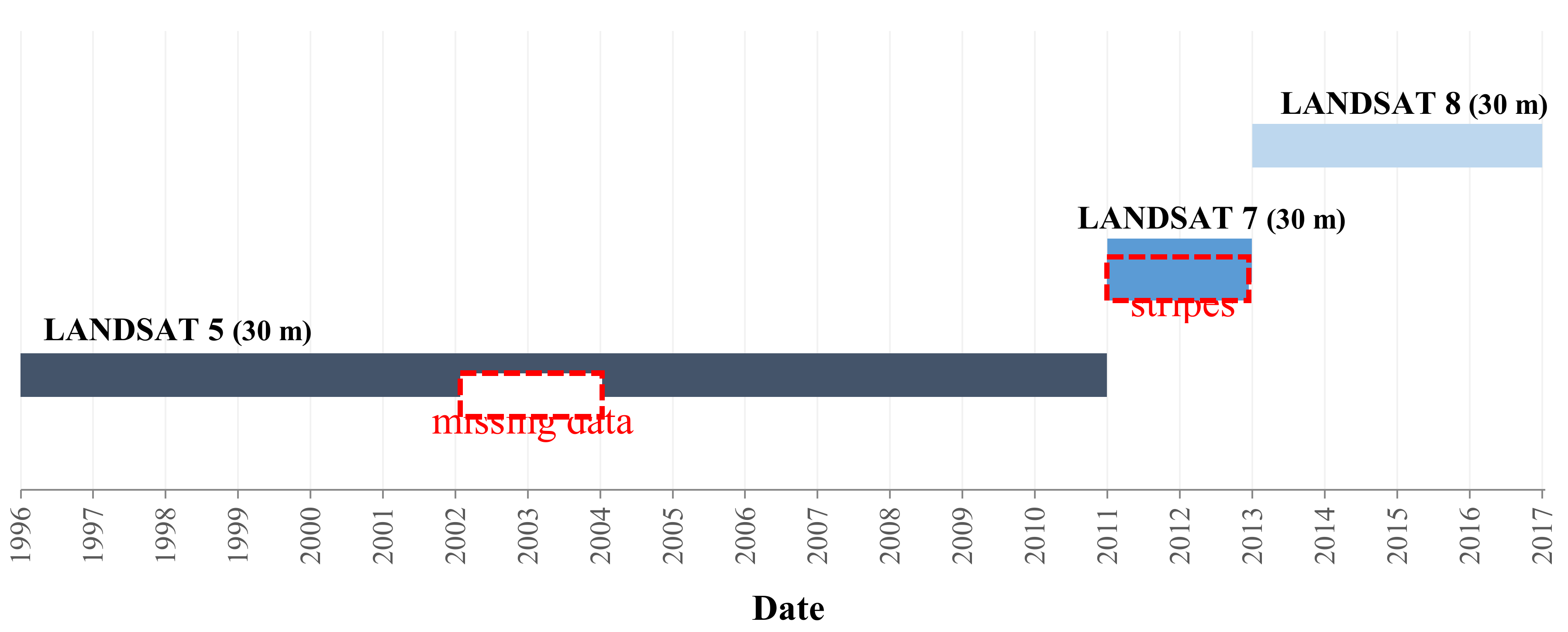
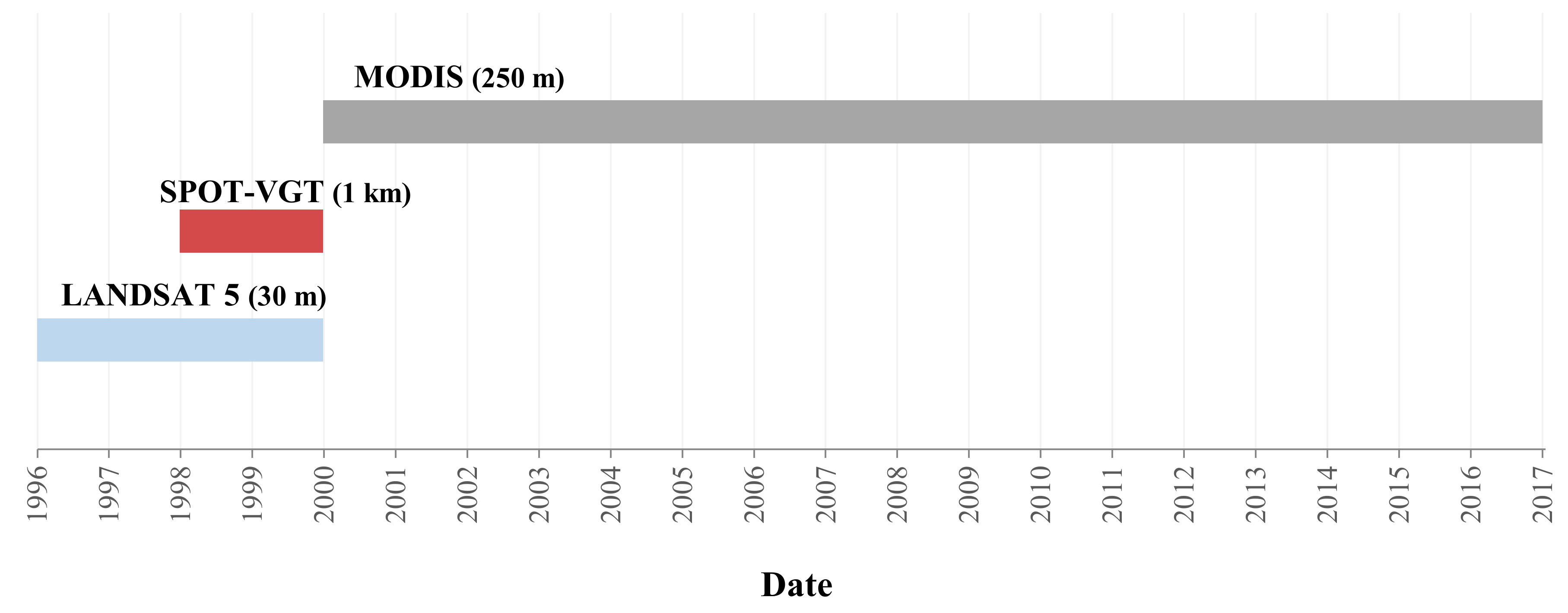
| NDVI data | 482 | MODIS (411), Landsat 5 TM (42), SPOT-Vegetation (29) |
| NDVI-biomass regression/validation | 3 | Sentinel-2, Landsat 8 OLI |
| Tile n. | Points | Product ID | Accuracy |
|---|---|---|---|
| 1 | 100 | 170067 | 0.93 |
| 2 | 100 | 170070 | 0.96 |
| 3 | 100 | 171069 | 0.93 |
| 4 | 100 | 172067 | 0.89 |
| 5 | 100 | 172071 | 0.85 |
| 6 | 100 | 173069 | 0.92 |
| 7 | 100 | 174071 | 0.91 |
| 8 | 100 | 175070 | 0.94 |
| average | 0.92 |
| Classified Data | ||||||||
|---|---|---|---|---|---|---|---|---|
| Forest/trees | Shrubland | Grassland | Bare soil | Water | Total | Producer’s Accuracy | ||
| reference data | forest/trees | 230 | 6 | 0 | 0 | 1 | 237 | 0.97 |
| shrubland | 2 | 179 | 3 | 11 | 0 | 195 | 0.92 | |
| grassland | 0 | 5 | 92 | 2 | 2 | 101 | 0.91 | |
| bare soil | 0 | 23 | 1 | 154 | 0 | 178 | 0.87 | |
| water | 0 | 0 | 5 | 0 | 84 | 89 | 0.94 | |
| total | 232 | 213 | 101 | 167 | 87 | 800 | - | |
| user’s accuracy | 0.99 | 0.84 | 0.91 | 0.92 | 0.97 | - | 0.92 | |
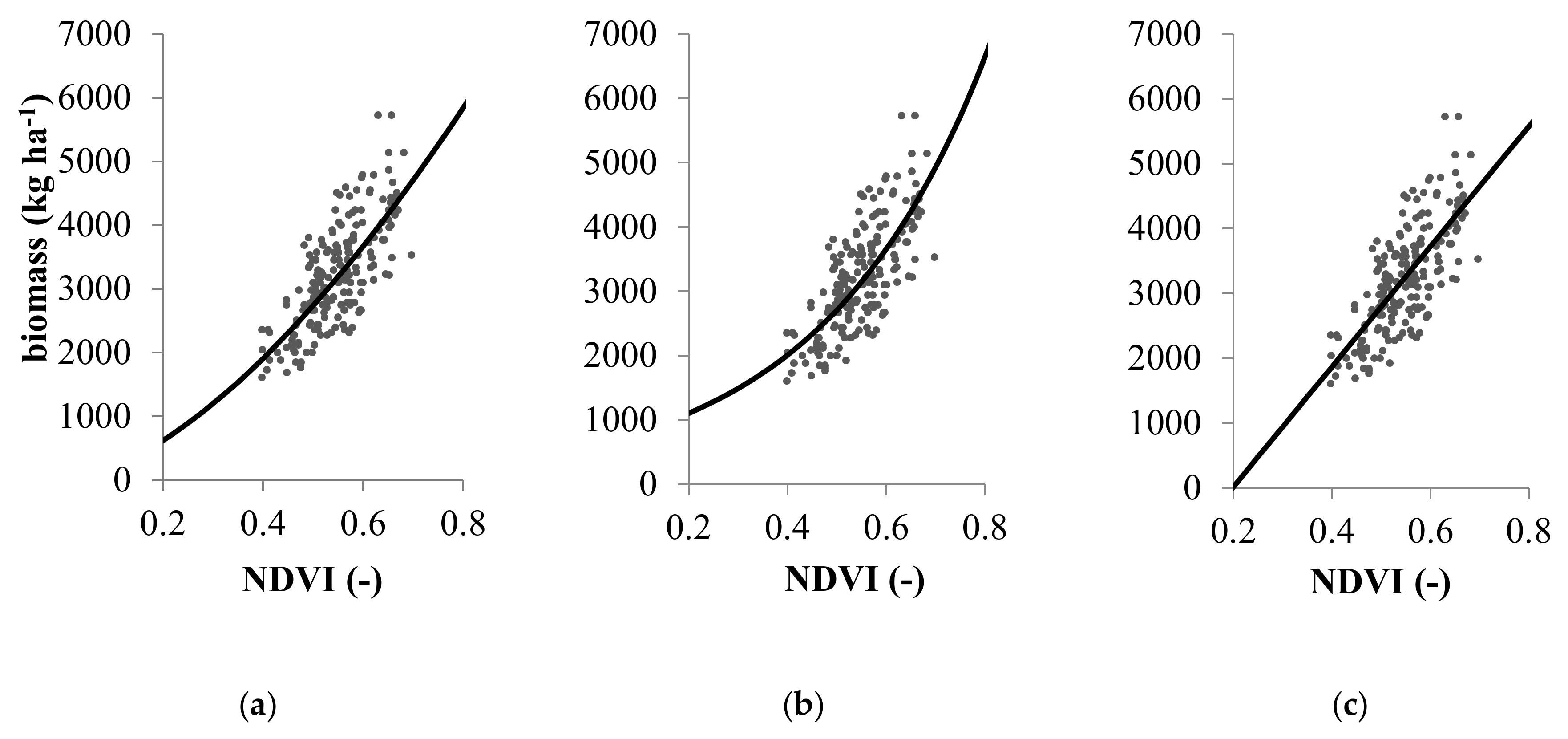
| Model | Equation | RMSE (kg ha−1) | MAE (kg ha−1) | REE (-) |
|---|---|---|---|---|
| Linear | −1838.10 + 9277.11 × NDVI | 572.54 | 460.16 | 0.171 |
| Power | 8373.59 × NDVI^1.61 | 572.29 | 457.86 | 0.169 |
| Exponential | 610.19 × exp(2.99 × NDVI) | 580.28 | 464.44 | 0.175 |
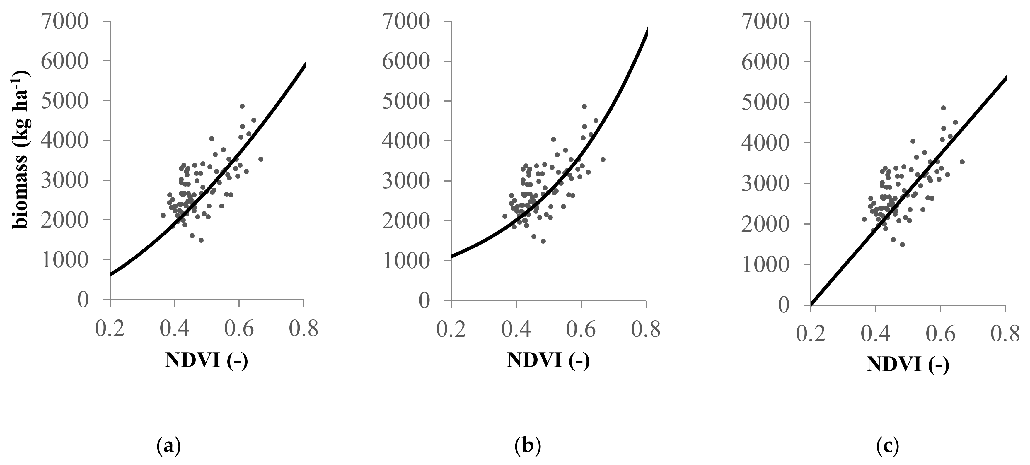
| Model | Equation | RMSE (kg ha−1) | MAE (kg ha−1) | REE (-) |
|---|---|---|---|---|
| Linear | −1838.10 + 9277.11 × NDVI | 570.12 | 459.42 | 0.238 |
| Power | 8373.59 × NDVI^1.61 | 539.73 | 426.62 | 0.214 |
| Exponential | 610.19 × exp(2.99*NDVI) | 562.89 | 449.82 | 0.233 |
| σ Landsat 5 | σ SPOT-VGT | σ MODIS | |
|---|---|---|---|
| Patch 1 | 0.107 | 0.066 | 0.089 |
| Patch 2 | 0.109 | 0.076 | 0.090 |
| Patch 3 | 0.093 | 0.062 | 0.071 |
| Patch 4 | 0.102 | 0.065 | 0.074 |
| Year | Precipitation/Year (mm) | Average of Max (ton/ha) | Average of min (ton/ha) | Length of Max (Days) | Length of min (Days) |
|---|---|---|---|---|---|
| 2003 | 920.33 | 4.12 | 1.66 | 48 | 80 |
| 2004 | 1197.43 | 4.36 | 1.89 | 93 | 48 |
| 2005 | 601.55 | 3.94 | 1.59 | 16 | 128 |
© 2020 by the authors. Licensee MDPI, Basel, Switzerland. This article is an open access article distributed under the terms and conditions of the Creative Commons Attribution (CC BY) license (http://creativecommons.org/licenses/by/4.0/).
Share and Cite
Clementini, C.; Pomente, A.; Latini, D.; Kanamaru, H.; Vuolo, M.R.; Heureux, A.; Fujisawa, M.; Schiavon, G.; Del Frate, F. Long-Term Grass Biomass Estimation of Pastures from Satellite Data. Remote Sens. 2020, 12, 2160. https://doi.org/10.3390/rs12132160
Clementini C, Pomente A, Latini D, Kanamaru H, Vuolo MR, Heureux A, Fujisawa M, Schiavon G, Del Frate F. Long-Term Grass Biomass Estimation of Pastures from Satellite Data. Remote Sensing. 2020; 12(13):2160. https://doi.org/10.3390/rs12132160
Chicago/Turabian StyleClementini, Chiara, Andrea Pomente, Daniele Latini, Hideki Kanamaru, Maria Raffaella Vuolo, Ana Heureux, Mariko Fujisawa, Giovanni Schiavon, and Fabio Del Frate. 2020. "Long-Term Grass Biomass Estimation of Pastures from Satellite Data" Remote Sensing 12, no. 13: 2160. https://doi.org/10.3390/rs12132160
APA StyleClementini, C., Pomente, A., Latini, D., Kanamaru, H., Vuolo, M. R., Heureux, A., Fujisawa, M., Schiavon, G., & Del Frate, F. (2020). Long-Term Grass Biomass Estimation of Pastures from Satellite Data. Remote Sensing, 12(13), 2160. https://doi.org/10.3390/rs12132160