Change Detection within Remotely Sensed Satellite Image Time Series via Spectral Analysis


Abstract
1. Introduction
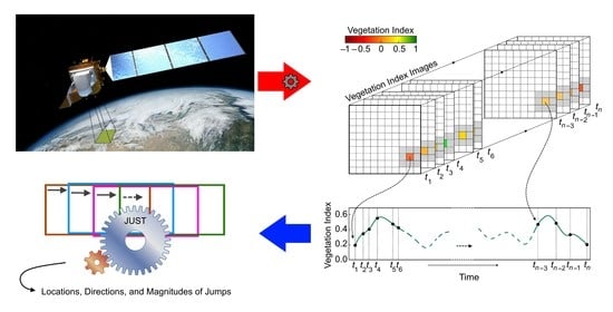
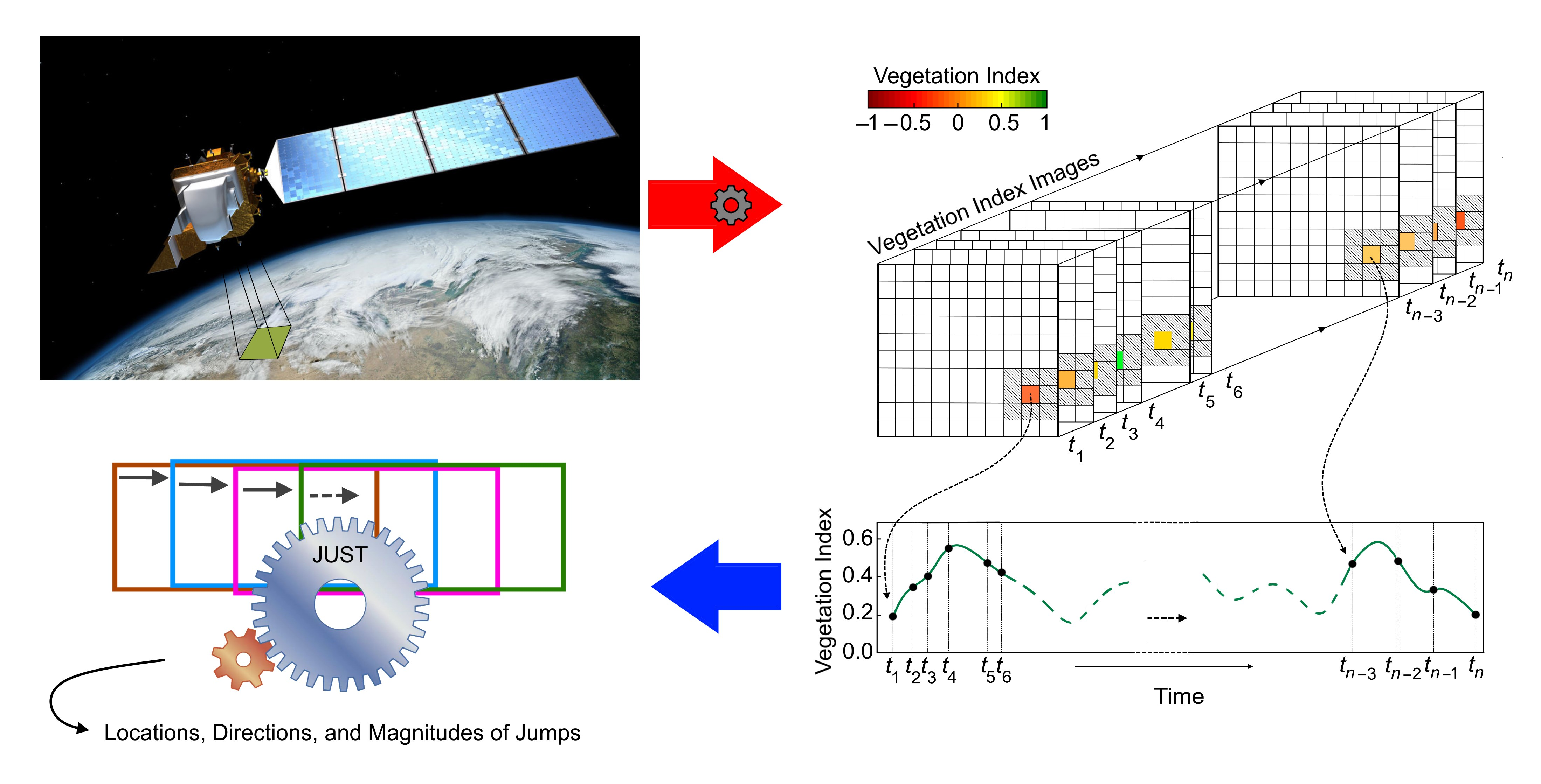
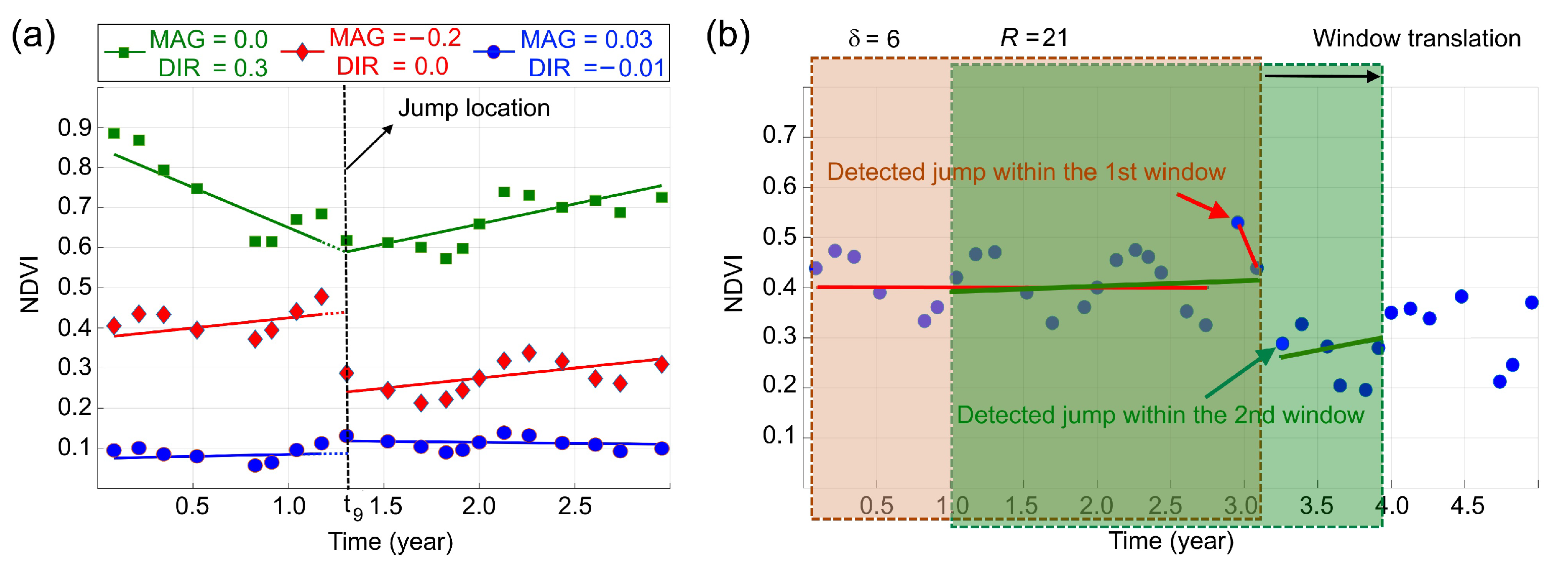
- The detection of jumps (sudden changes) in the trend component of an unequally spaced time series;
- Accounting for uncertainties in the time series values (observational uncertainties) to improve the estimation of trend and seasonal components, and jump locations; and
- The characterization of the gradual and sudden changes in the ecosystem by estimating the jump direction and magnitude.
2. Materials and Methods
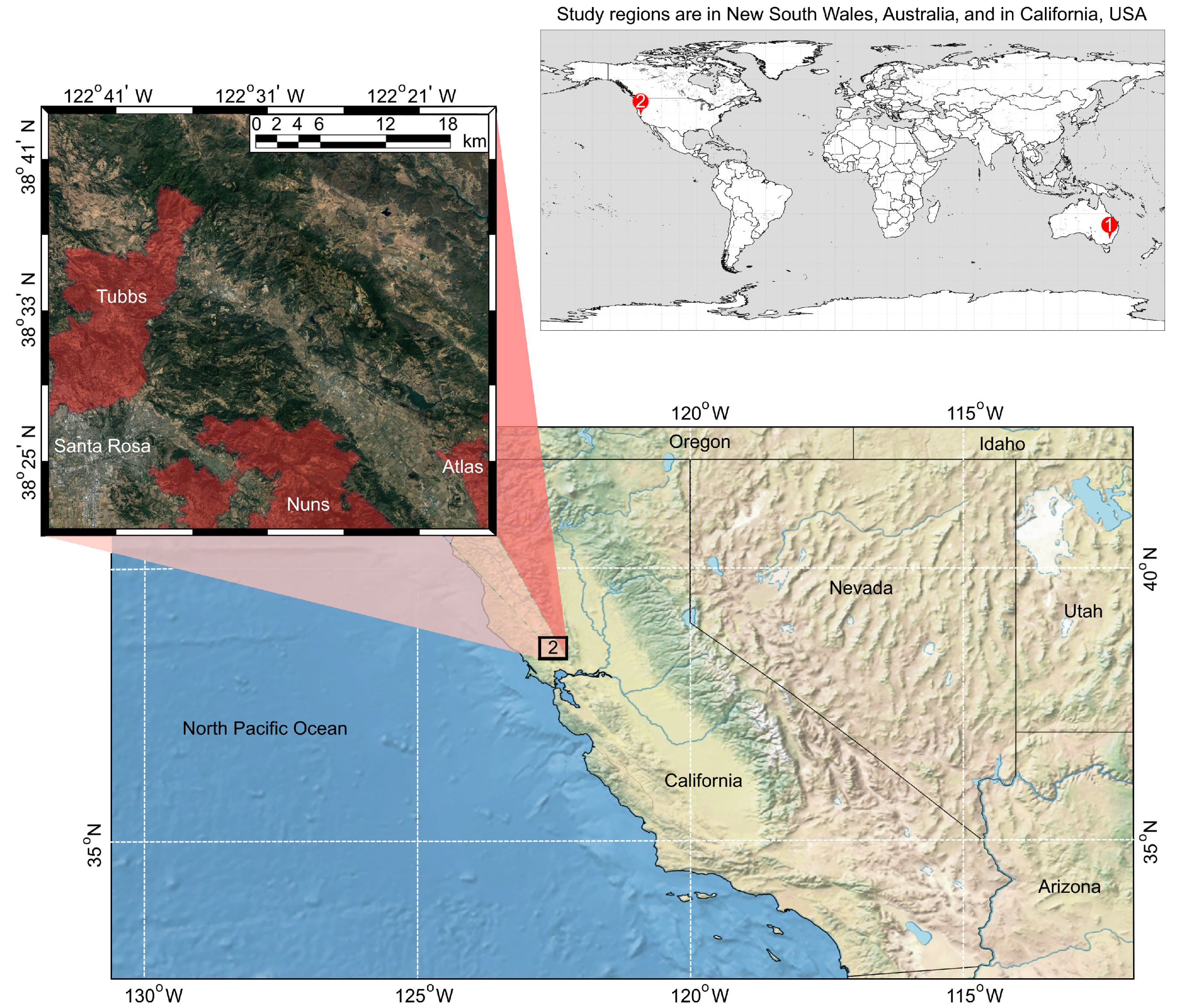
2.1. Study Regions
2.2. Data Sets and Pre-Processing
2.3. Weighted Vegetation Time Series
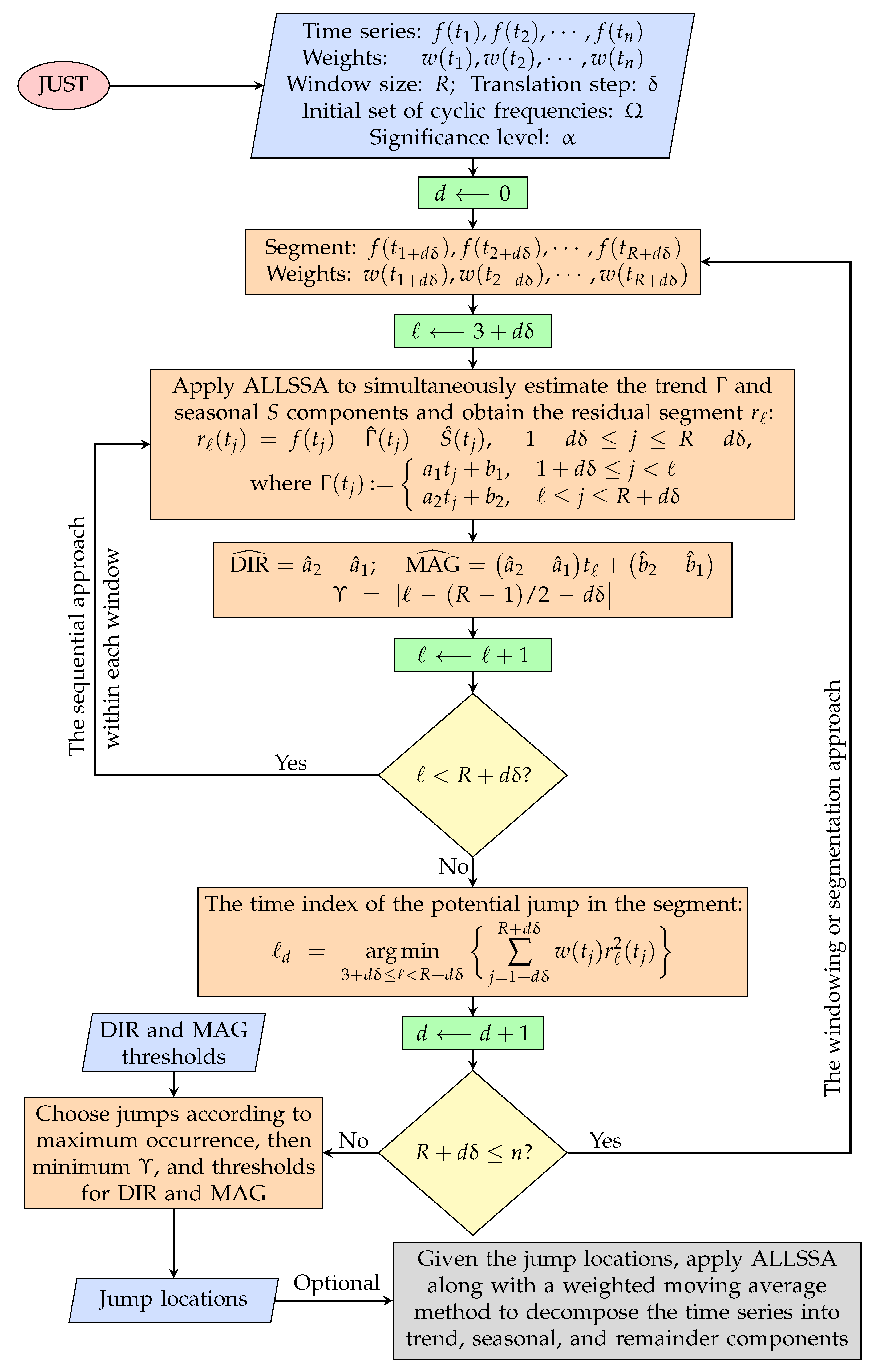
2.4. Jumps Upon Spectrum and Trend (JUST)
2.5. Breaks for Additive Seasonal and Trend (BFAST)
2.6. Validation through Descriptive Statistics
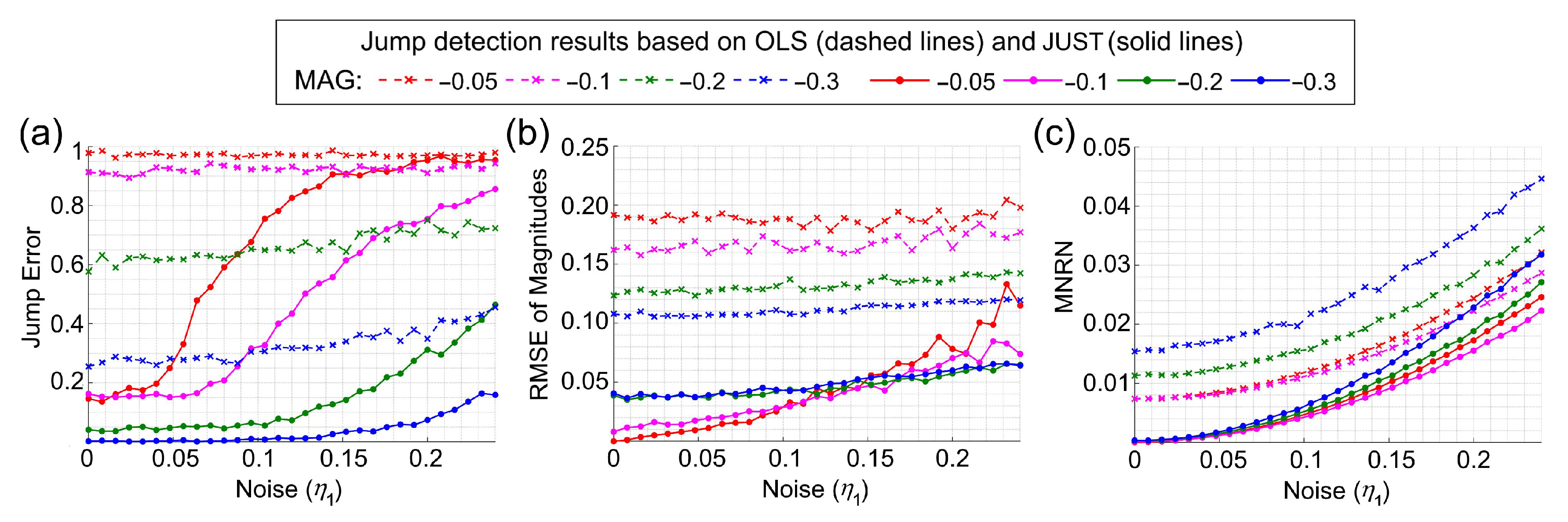
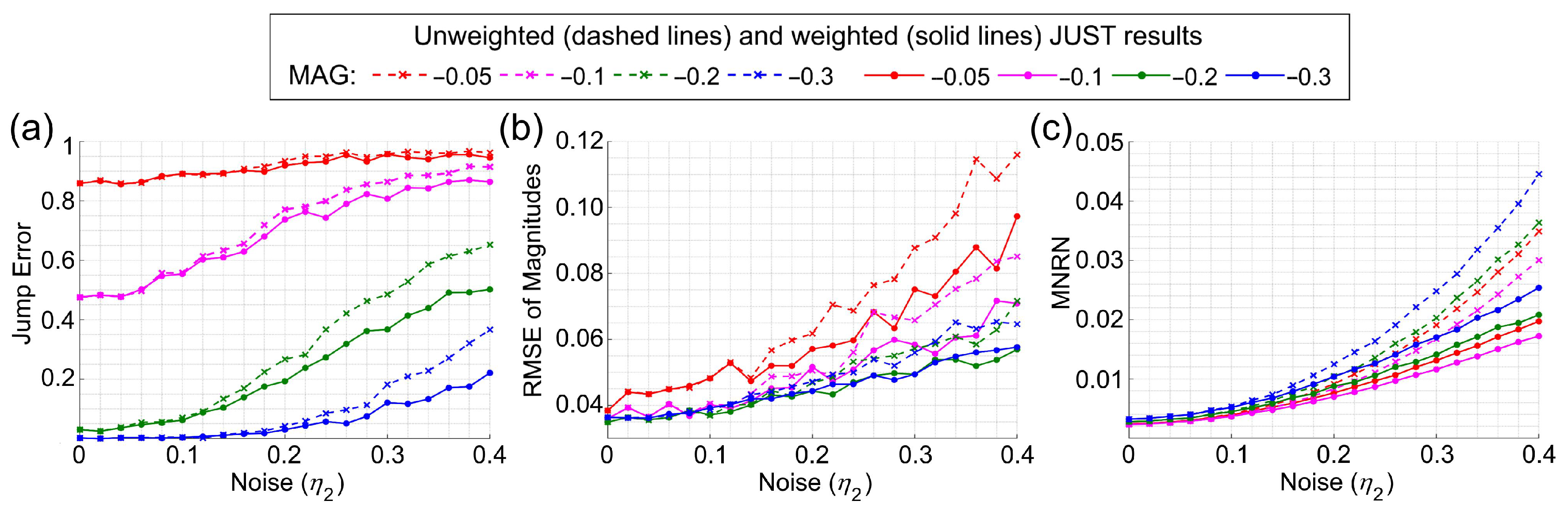
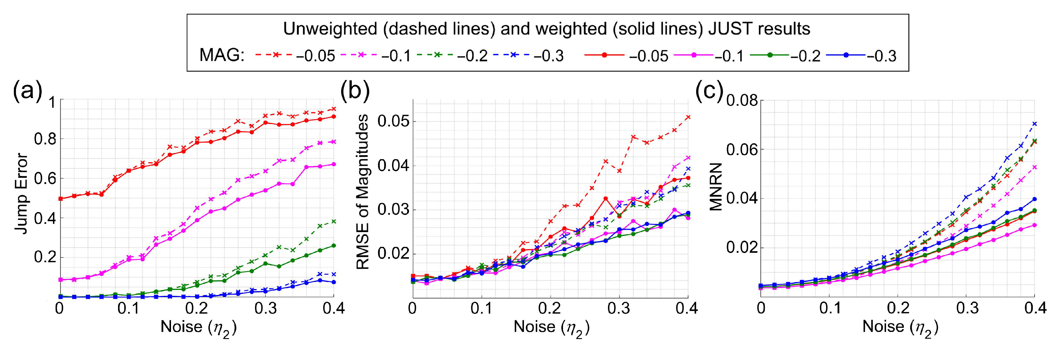
- Jump error for the K time series: the number of incorrectly detected jump locations divided by K, i.e., normalized.
- Root Mean Square Error (RMSE) for the jump magnitude when the jump location is correctly detected:where m is the number of correctly detected jump locations (), and are the true and estimated magnitudes of a correctly detected jump, respectively, see Equation (4).
- Mean Normalized Residual Norm (MNRN): compute the Normalized Residual Norm (NRN) for each of the K time series, then find their average. For a given time series, NRN is defined as the weighted L2 norm of estimated residual series divided by the weighted L2 norm of the original series. More precisely:where f is a time series with its associated weights w (if available), n is the number of observations, and r is the residual series obtained after subtracting the estimated trend and seasonal components from f.
3. Results and Discussion
3.1. Simulation Experiment
3.1.1. Simulation of Time Series with Unknown Seasonality
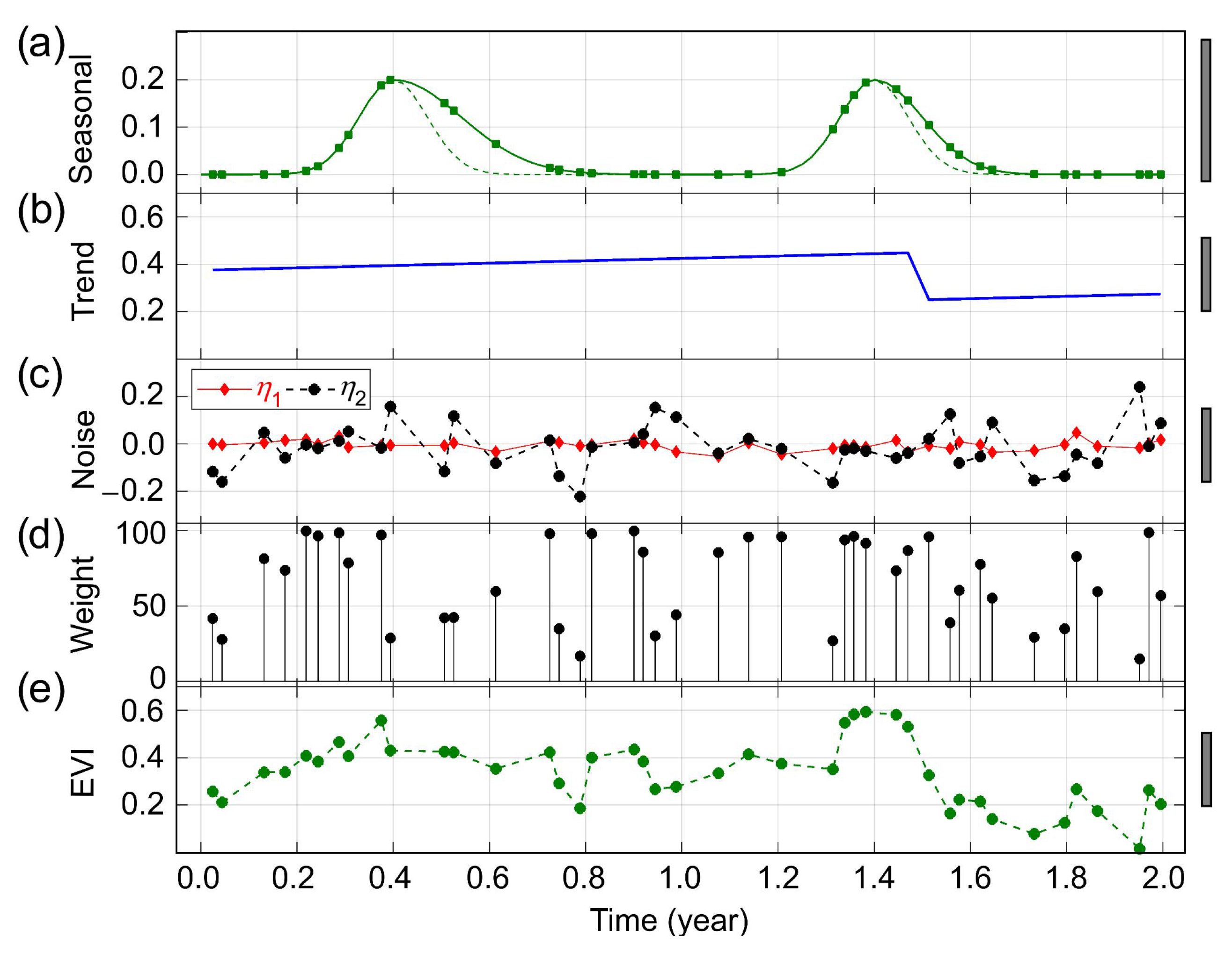
3.1.2. Simulation of Time Series with Two Noises of the Same Type
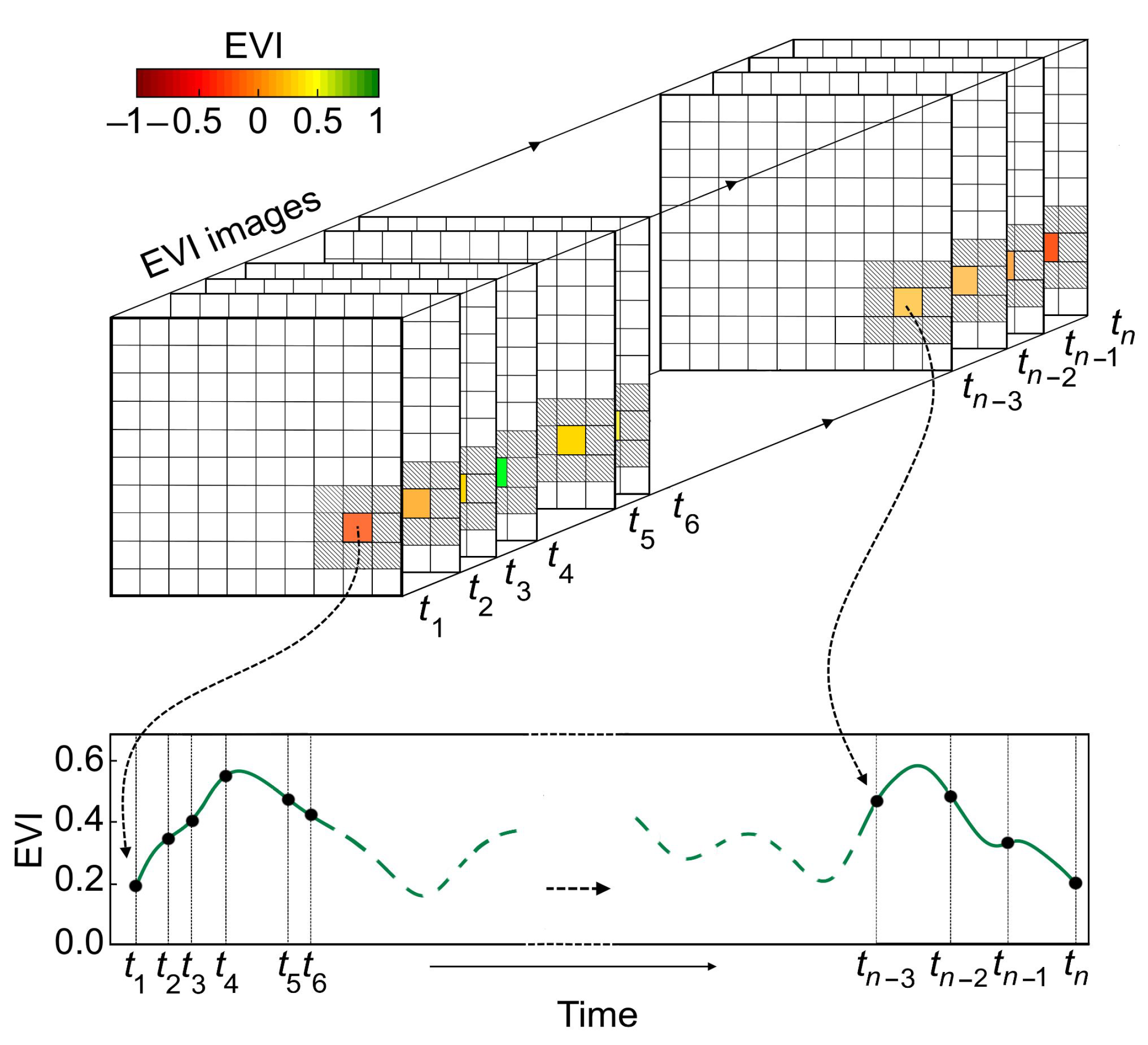
3.1.3. A Simulated EVI Time Series with Multiple Jumps
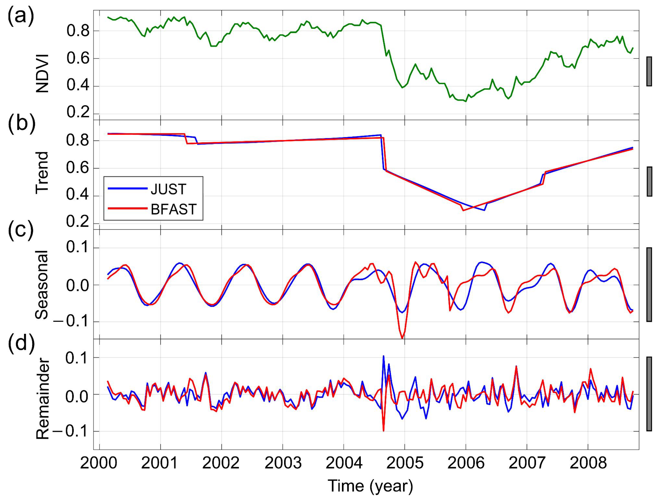
3.2. Detecting and Characterizing Jumps in the NDVI Time Series for the First Study Region
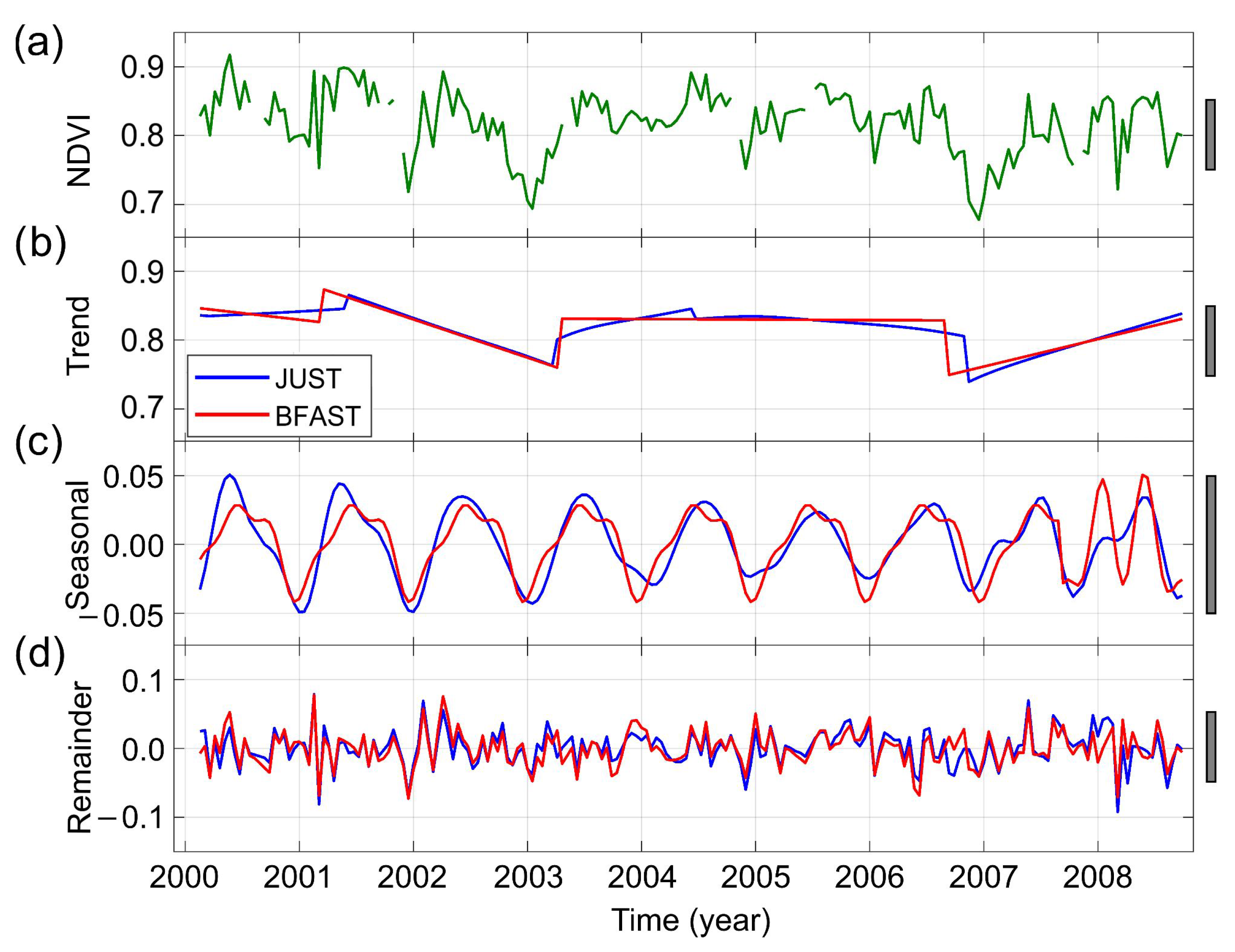
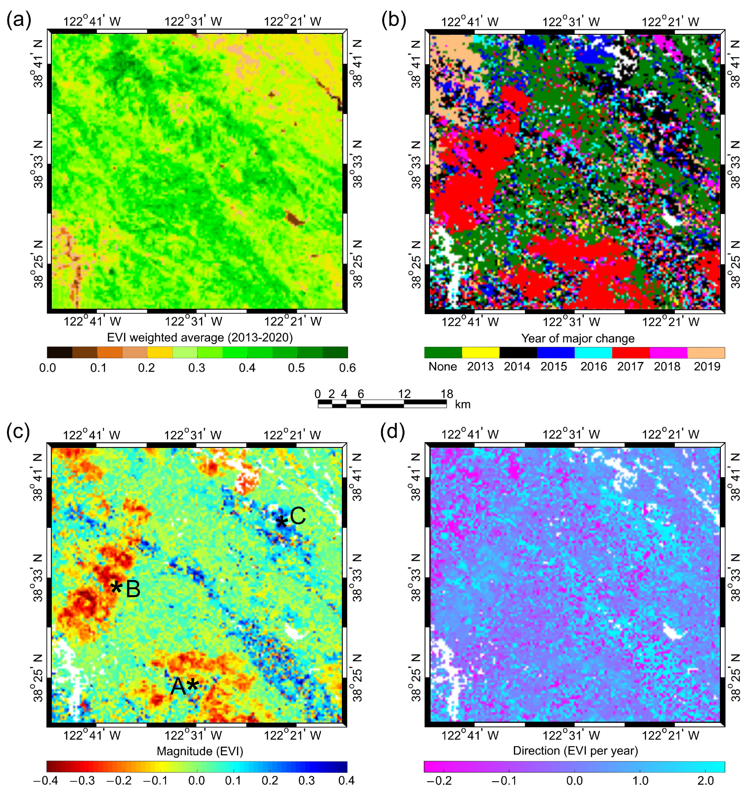
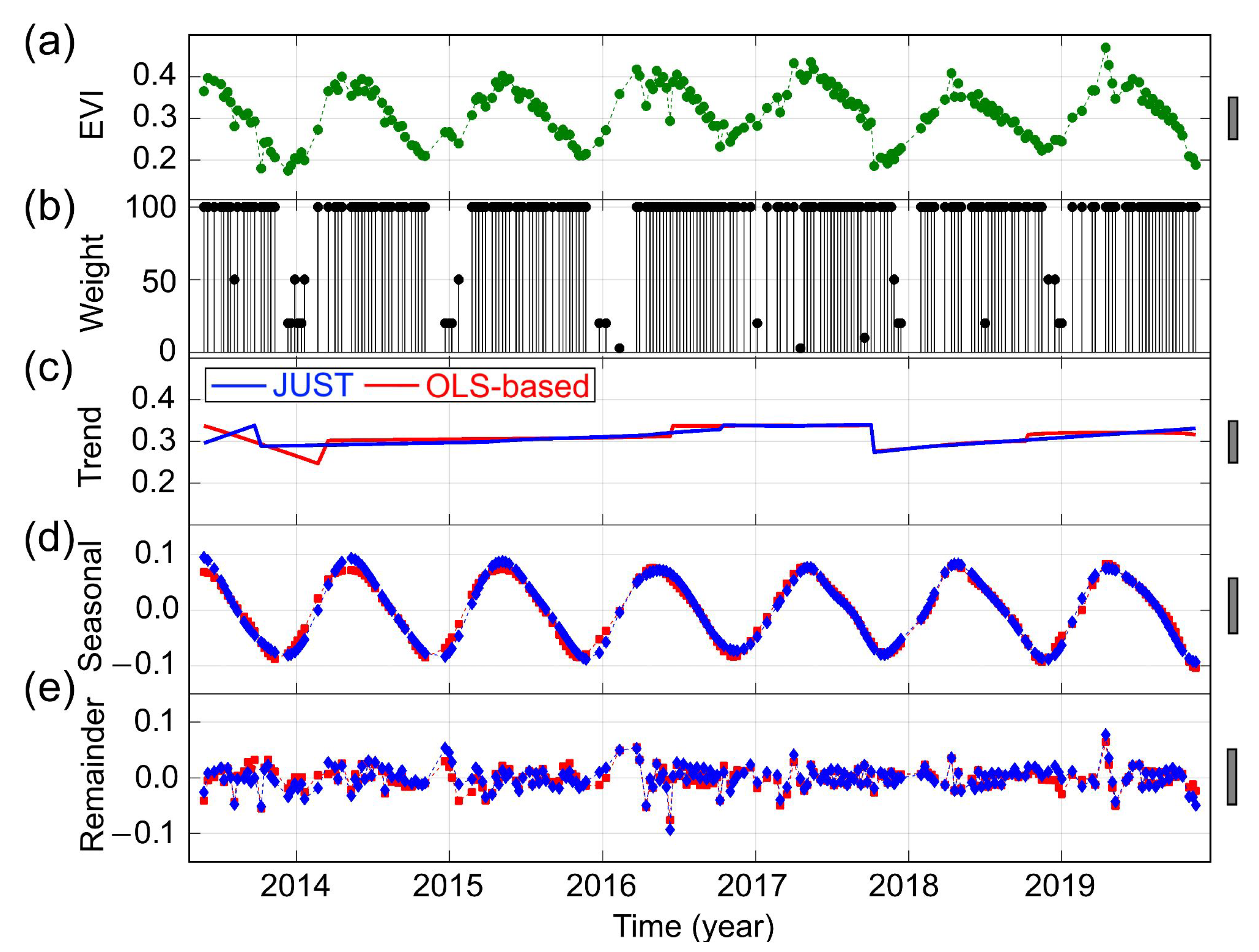
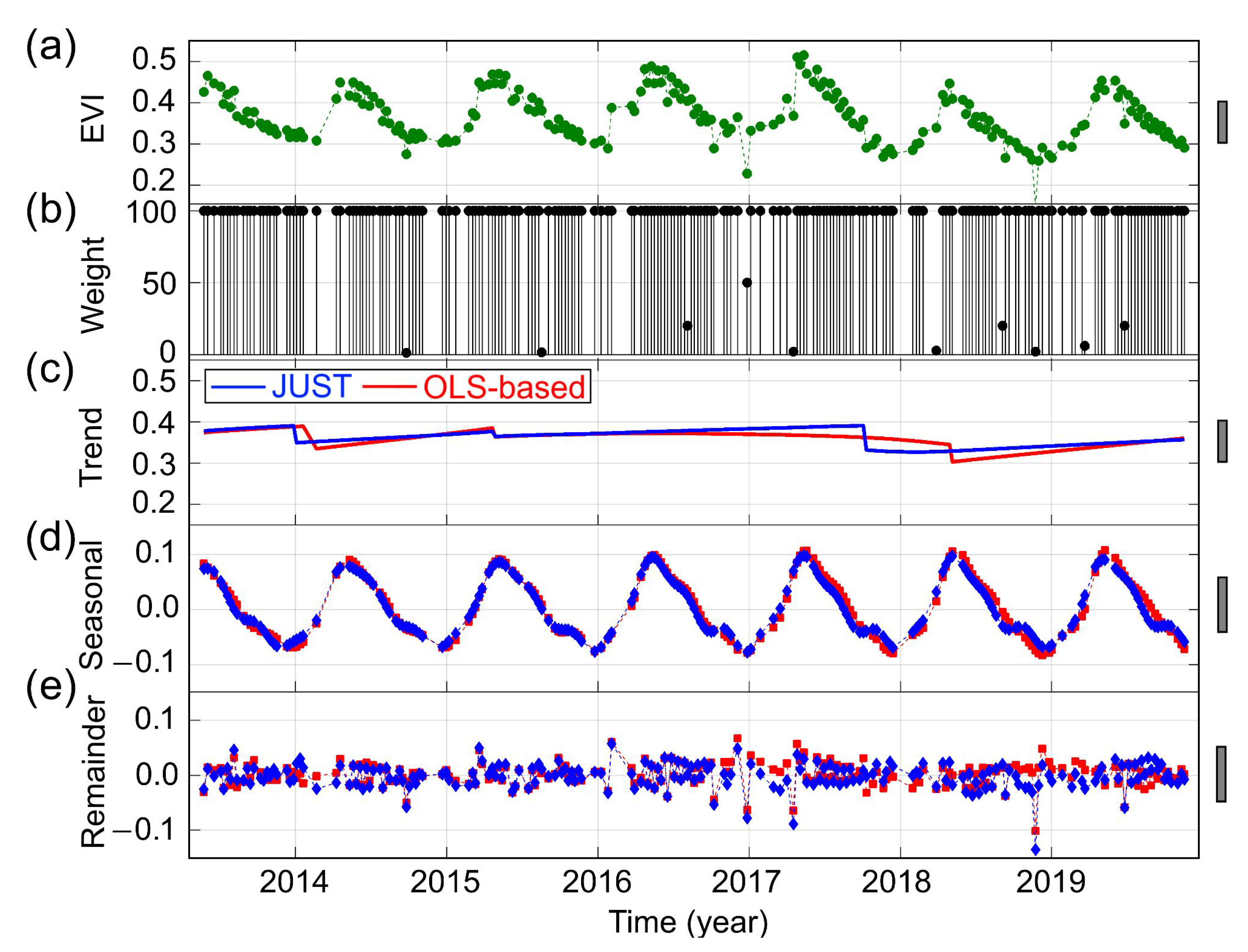
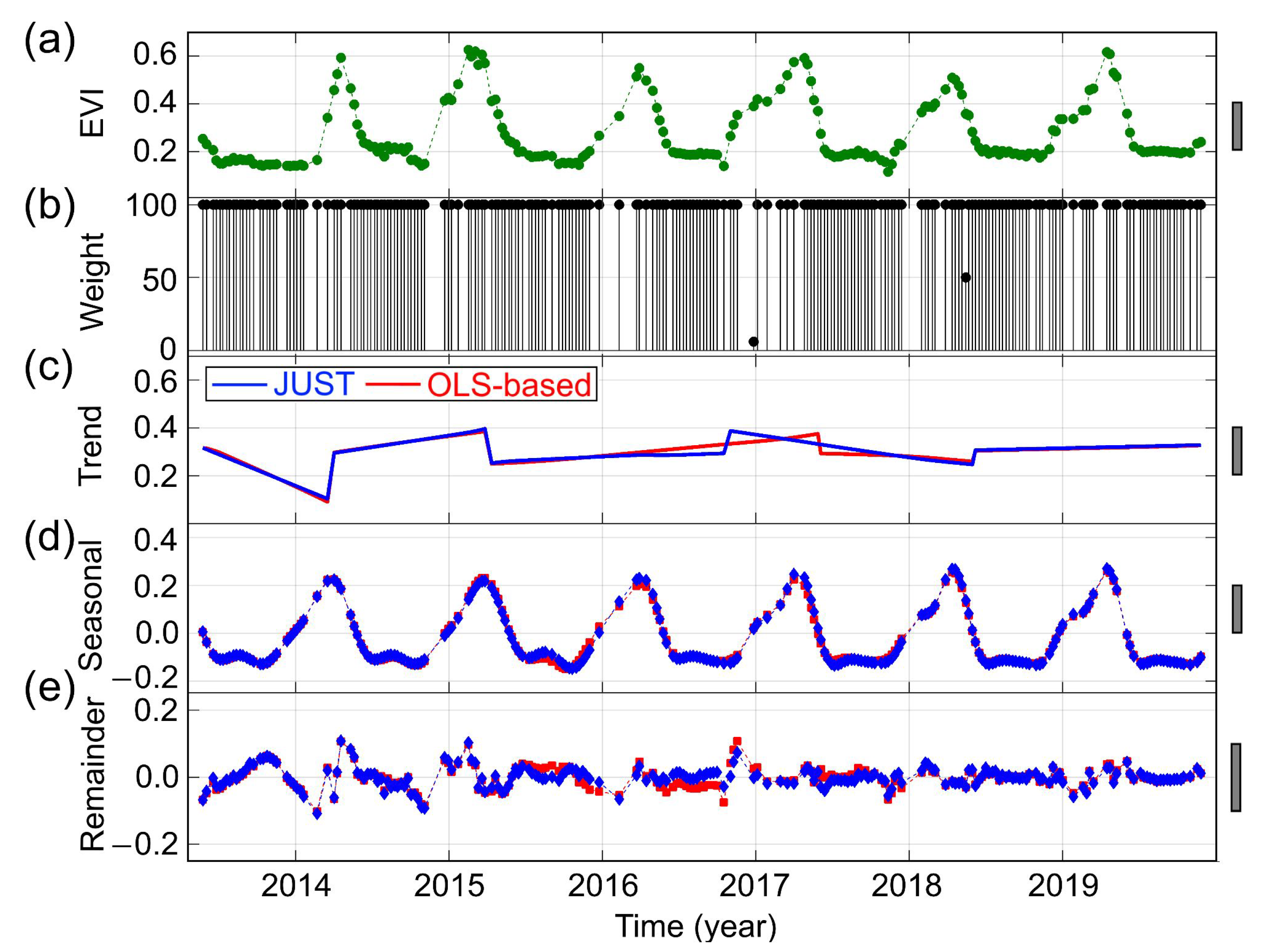
3.3. Detecting and Characterizing Jumps in the Landsat 8 Image Time Series for the Second Study Region
4. Conclusions and Future Work
Author Contributions
Funding
Acknowledgments
Conflicts of Interest
Abbreviations
| ALLSSA | Anti-Leakage Least-Squares Spectral Analysis |
| BFAST | Breaks For Additive Seasonal and Trend |
| CCDC | Continuous Change Detection and Classification |
| DBEST | Detecting Breakpoints and Estimating Segments in Trend |
| EVI | Enhanced Vegetation Index |
| JUST | Jumps Upon Spectrum and Trend |
| LSWA | Least-Squares Wavelet Analysis |
| LSWAVE | Least-Squares Wavelet (software) |
| MNRN | Mean Normalized Residual Norm |
| MODIS | Moderate Resolution Imaging Spectroradiometer |
| NASA | National Aeronautics and Space Administration |
| NDVI | Normalized Difference Vegetation Index |
| OLS | Ordinary Least-Squares |
| OLS-MOSUM | Ordinary Least-Squares Residuals-Based Moving Sum |
| PQA | Pixel Quality Assessment |
| RMSE | Root Mean Square Error |
| STL | Seasonal-Trend decomposition procedure based on Loess |
| TOA | Top Of Atmosphere |
| USGS | U.S. Geological Survey |
References
- DeFries, R.S.; Field, C.B.; Fung, I.; Collatz, G.J.; Bounoua, L. Combining satellite data and biogeochemical models to estimate global effects of human-induced land cover change on carbon emissions and primary productivity. Glob. Biogeochem. Cycles 1999, 13, 803–815. [Google Scholar] [CrossRef]
- Luo, L.; Wood, E.F. Monitoring and predicting the 2007 U.S. drought. Geophys. Res. Lett. 2007, 34, 6. [Google Scholar] [CrossRef]
- Akther, M.S.; Hassan, Q.K. Remote sensing-based assessment of fire danger conditions over boreal forest. IEEE J. Sel. Top. Appl. Earth Obs. Remote Sens. 2011, 4, 992–999. [Google Scholar] [CrossRef]
- Farjad, B.; Gupta, A.; Sartipizadeh, H.; Cannon, A.J. A novel approach for selecting extreme climate change scenarios for climate change impact studies. Sci. Total Environ. 2019, 678, 476–485. [Google Scholar] [CrossRef]
- Zhang, K.; Thapa, B.; Ross, M.; Gann, D. Remote sensing of seasonal changes and disturbances in mangrove forest: A case study from South Florida. Ecosphere 2016, 7, 1–23. [Google Scholar] [CrossRef]
- Xu, Y.; Yu, L.; Cai, Z.; Zhao, J.; Peng, D.; Li, C.; Lu, H.; Yu, C.; Gong, P. Exploring intra-annual variation in cropland classification accuracy using monthly, seasonal, and yearly sample set. Int. J. Remote Sens. 2019, 40, 8748–8763. [Google Scholar] [CrossRef]
- Verbesselt, J.; Hyndman, R.; Zeileis, A.; Culvenor, D. Phenological change detection while accounting for abrupt and gradual trends in satellite image time series. Remote Sens. Environ. 2010, 114, 2970–2980. [Google Scholar] [CrossRef]
- Verbesselt, J.; Hyndman, R.; Newnham, G.; Culvenor, D. Detecting trend and seasonal changes in satellite image time series. Remote Sens. Environ. 2010, 114, 106–115. [Google Scholar] [CrossRef]
- Rouse, J.W.; Hass, R.H., Jr.; Schell, J.A.; Deering, D.W. Monitoring vegetation systems in the great plains with ERTS. In Proceedings of the Third Earth Resources Technology Satellite-1 Symposium 1 (A), Texas A&M University, College Station, TX, USA, 1 January 1974; pp. 309–317. [Google Scholar]
- Liu, H.Q.; Huete, A. A feedback based modification of the NDVI to minimize canopy background and atmospheric noise. IEEE Trans. Geosci. Remote Sens. 1995, 33, 457–465. [Google Scholar] [CrossRef]
- Matsushita, B.; Yang, W.; Chen, J.; Onda, Y.; Qiu, G. Sensitivity of the Enhanced Vegetation Index (EVI) and Normalized Difference Vegetation Index (NDVI) to topographic effects: A case study in high-density Cypress forest. Sensors 2007, 7, 2636–2651. [Google Scholar] [CrossRef] [PubMed]
- Ware, A.F. Fast approximate Fourier transforms for irregularly spaced data. SIAM Rev. 1988, 40, 838–856. [Google Scholar] [CrossRef]
- Mallat, S. A Wavelet Tour of Signal Processing; Academic Press: Cambridge, UK, 1999. [Google Scholar]
- Percival, D.B.; Wang, M.; Overland, J.E. An introduction to wavelet analysis with applications to vegetation time series. Community Ecol. 2004, 5, 19–30. [Google Scholar] [CrossRef]
- Press, W.H.; Teukolsky, A. Search algorithm for weak signals in unevenly spaced data. Comput. Phys. 1988, 2, 77–82. [Google Scholar] [CrossRef]
- Samanta, A.; Costa, M.H.; Nunes, E.L.; Vieira, S.A.; Xu, L.; Myneni, R.B. Comment on “Drought-Induced Reduction in Global Terrestrial Net Primary Production from 2000 Through 2009”. Science 2011, 333, 1093. [Google Scholar] [CrossRef]
- Zhu, Z.; Wang, S.; Woodcock, C.E. Improvement and expansion of the Fmask algorithm: Cloud, cloud shadow, and snow detection for Landsats 4–7, 8, and Sentinel 2 images. Remote Sens. Environ. 2015, 159, 269–277. [Google Scholar] [CrossRef]
- Jeppesen, J.H.; Jacobsen, R.H.; Inceoglu, F.; Toftegaard, T.S. A cloud detection algorithm for satellite imagery based on deep learning. Remote Sens. Environ. 2019, 229, 247–259. [Google Scholar] [CrossRef]
- Shao, Z.; Pan, Y.; Diao, C.; Cai, J. Cloud detection in remote sensing images based on multiscale features-convolutional neural network. IEEE Trans. Geosci. Remote Sens. 2019, 57, 4062–4076. [Google Scholar] [CrossRef]
- Zhang, X.Y.; Friedl, M.A.; Schaaf, C.B. Sensitivity of vegetation phenology detection to the temporal resolution of satellite data. Int. J. Remote Sens. 2009, 30, 2061–2074. [Google Scholar] [CrossRef]
- Ghaderpour, E.; Vujadinovic, T. The Potential of the Least-Squares Spectral and Cross-Wavelet Analyses for Near-Real-Time Disturbance Detection within Unequally Spaced Satellite Image Time Series. Remote Sens. 2020, 12, 2446. [Google Scholar] [CrossRef]
- Ghaderpour, E. Least-Squares Wavelet Analysis and Its Applications in Geodesy and Geophysics. Ph.D. Thesis, York University, Toronto, ON, Canada, 2018. [Google Scholar]
- Zhu, Z.; Woodcock, C.E. Continuous change detection and classification of land cover using all available Landsat data. Remote Sens. Environ. 2014, 144, 152–171. [Google Scholar] [CrossRef]
- Cleveland, R.B.; Cleveland, W.S.; McRae, J.E.; Terpenning, I. STL: A seasonal-trend decomposition procedure based on loess. J. Off. Stat. 1990, 6, 3–73. [Google Scholar]
- Brandt, M.; Verger, A.; Diouf, A.A.; Baret, F.; Samimi, C. Local vegetation trends in the Sahel of Mali and Senegal using long time series FAPAR satellite products and field measurement (1982–2010). Remote Sens. 2014, 6, 2408–2434. [Google Scholar] [CrossRef]
- Jamali, S.; Jönsson, P.; Eklundh, L.; Ardö, J.; Seaquist, J. Detecting changes in vegetation trends using time series segmentation. Remote Sens. Environ. 2015, 156, 182–195. [Google Scholar] [CrossRef]
- Rodionov, S.N. A sequential algorithm for testing climate regime shifts. Geophys. Res. Lett. 2004, 31, L09204. [Google Scholar] [CrossRef]
- Aminikhanghahi, S.; Cook, D.J. A survey of methods for time series change point detection. Knowl. Inf. Syst. 2017, 51, 339–367. [Google Scholar] [CrossRef]
- Khan, S.H.; He, X.; Porikli, F.; Bennamoun, M. Forest change detection in incomplete satellite images with deep neural networks. IEEE Trans. Geosci. Remote Sens. 2017, 55, 5407–5423. [Google Scholar] [CrossRef]
- Ghaderpour, E.; Pagiatakis, S.D. Least-squares wavelet analysis of unequally spaced and non-stationary time series and its applications. Math. Geosci. 2017, 49, 819–844. [Google Scholar] [CrossRef]
- Ghaderpour, E.; Liao, W.; Lamoureux, M.P. Antileakage least-squares spectral analysis for seismic data regularization and random noise attenuation. Geophysics 2018, 8, V157–V170. [Google Scholar] [CrossRef]
- Ghaderpour, E.; Pagiatakis, S.D. LSWAVE: A MATLAB software for the least-squares wavelet and cross-wavelet analyses. GPS Solut. 2019, 23, 8. [Google Scholar] [CrossRef]
- LSWAVE: A MATLAB Software for the Least-Squares Wavelet and Cross-Wavelet Analyses–by E. Ghaderpour and S. D. Pagiatakis. National Geodetic Survey (NGS)—National Oceanic and Atmospheric Administration (NOAA). Available online: https://www.ngs.noaa.gov/gps-toolbox/LSWAVE.htm (accessed on 1 October 2020).
- Ghaderpour, E.; Ben Abbes, A.; Rhif, M.; Pagiatakis, S.D.; Farah, I.R. Non-stationary and unequally spaced NDVI time series analyses by the LSWAVE software. Int. J. Remote Sens. 2019, 41, 2374–2390. [Google Scholar] [CrossRef]
- Forkel, M.; Carvalhais, N.; Verbesselt, J.; Mahecha, M.D.; Neigh, C.S.R.; Reichstein, M. Trend change detection in NDVI time series: Effects of inter-annual variability and methodology. Remote Sens. 2013, 5, 2113–2144. [Google Scholar] [CrossRef]
- Watts, L.M.; Laffan, S.W. Effectiveness of the BFAST algorithm for detecting vegetation response patterns in a semi-arid region. Remote Sens. Environ. 2014, 154, 234–245. [Google Scholar] [CrossRef]
- Zhu, Z. Change detection using Landsat time series: A review of frequencies, preprocessing, algorithms, and applications. ISPRS J. Photogramm. Remote Sens. 2017, 130, 370–384. [Google Scholar] [CrossRef]
- Ben Abbes, A.; Bounouh, O.; Farah, I.R.; de Jong, R.; Martinez, B. Comparative study of three satellite image time-series decomposition methods for vegetation change detection. Eur. J. Remote Sens. 2018, 61, 607–615. [Google Scholar] [CrossRef]
- Awty-Carroll, K.; Bunting, P.; Hardy, A.; Bell, G. An evaluation and comparison of four dense time series change detection methods using simulated data. Remote Sens. 2019, 11, 2779. [Google Scholar] [CrossRef]
- Stuart, J.D.; Sawyer, J.O. Trees and Shrubs of California; University of California Press: Berkeley, CA, USA, 2001. [Google Scholar]
- Lightfoot, K.G.; Parrish, O. California Indians and Their Environment: An Introduction; University of California Press: Berkeley, CA, USA, 2009. [Google Scholar]
- Li, A.X.; Wang, Y.; Yung, Y.L. Inducing factors and impacts of the October 2017 California wildfires. Earth Space Sci. 2019, 6, 1480–1488. [Google Scholar] [CrossRef]
- Monitoring Trends in Burn Severity: Fire Occurrence Locations and Burned Area Boundaries. Available online: https://apps.fs.usda.gov/arcx/rest/services/EDW/EDW_MTBS_01/MapServer (accessed on 1 October 2020).
- Runge, A.; Grosse, G. Comparing Spectral Characteristics of Landsat-8 and Sentinel-2 Same-Day Data for Arctic-Boreal Regions. Remote Sens. 2019, 11, 1730. [Google Scholar] [CrossRef]
- Breaks for Additive Seasonal and Trend (BFAST) R-Code. Available online: https://cran.r-project.org/web/packages/bfast/index.html (accessed on 1 October 2020).
- Shorthouse, D.P. SimpleMappr, An Online Tool to Produce Publication-Quality Point Maps. 2019. Available online: https://www.simplemappr.net (accessed on 13 November 2020).
- USGS—Science for a Changing World—Earth Explorer. Available online: https://earthexplorer.usgs.gov/ (accessed on 1 October 2020).
- Roy, D.P.; Wulder, M.A.; Loveland, T.R.; Woodcock, C.E.; Allen, R.G.; Anderson, M.C.; Helderg, D.; Ironsh, J.R.; Johnsoni, D.M.; Kennedy, R.; et al. Landsat-8: Science and product vision for terrestrial global change research. Remote Sens. Environ. 2014, 145, 154–172. [Google Scholar] [CrossRef]
- Kovalskyy, V.; Roy, D.P. The global availability of Landsat 5 TM and Landsat 7 ETM+ land surface observations and implications for global 30m Landsat data product generation. Remote Sens. Environ. 2013, 130, 280–293. [Google Scholar] [CrossRef]
- Loveland, T.R.; Dwyer, J.L. Landsat: Building a strong future. Remote Sens. Environ. 2012, 122, 22–29. [Google Scholar] [CrossRef]
- She, X.; Zhang, L.; Cen, Y.; Wu, T.; Huang, C.; Baig, M.H.A. Comparison of the continuity of vegetation indices derived from Landsat 8 OLI and Landsat 7 ETM+ data among different vegetation types. Remote Sens. 2015, 7, 13485–13506. [Google Scholar] [CrossRef]
- Huete, A.; Didan, K.; Miura, T.; Rodriguez, E.P.; Gao, X.; Ferreira, L.G. Overview of the radiometric and biophysical performance of the MODIS vegetation indices. Remote Sens. Environ. 2002, 83, 195–213. [Google Scholar] [CrossRef]
- Wells, D.E.; Krakiwsky, E.J. The Method of Least-Squares; Department of Surveying Engineering, University of New Brunswick: Fredericton, NB, Canada, 1971. [Google Scholar]
- Foster, G. Wavelet for period analysis of unevenly sampled time series. Astron. J. 1996, 112, 1709–1729. [Google Scholar] [CrossRef]
- Motohka, T.; Nasahara, K.N.; Murakami, K.; Nagai, S. Evaluation of sub-pixel cloud noises on MODIS daily spectral indices based on in situ measurements. Remote Sens. 2011, 3, 1644–1662. [Google Scholar] [CrossRef]
- Bento, J. On the complexity of the weighted fused lasso. IEEE Signal Process. Lett. 2018, 25, 1595–1599. [Google Scholar] [CrossRef]
- Zhu, Z.; Woodcock, C.E.; Holden, C.; Yang, Z. Generating synthetic Landsat images based on all available Landsat data: Predicting Landsat surface reflectance at any given time. Remote Sens. Environ. 2015, 162, 67–83. [Google Scholar] [CrossRef]
- VanderPlas, J.T. Understanding the Lomb–Scargle Periodogram. Astrophys. J. Suppl. Ser. 2018, 236, 28. [Google Scholar] [CrossRef]
- Schwartz, M.D. Advancing to full bloom: Planning phenological research for the 21st century. Int. J. Biometeorol. 1999, 42, 113–118. [Google Scholar] [CrossRef]
- Zeileis, A. A unified approach to structural change tests based on ML scores, F statistics, and OLS residuals. Econom. Rev. 2005, 24, 445–466. [Google Scholar] [CrossRef]
- Venables, W.N.; Ripley, B.D. Modern Applied Statistics with S-PLUS; Springer: Berlin, Germany, 2013. [Google Scholar]
- Verbesselt, J.; Zeileis, A.; Herold, M. Near real-time disturbance detection using satellite image time series. Remote Sens. Environ. 2012, 123, 98–108. [Google Scholar] [CrossRef]
- Özgür, C.; Colliau, T.; Rogers, G.; Hughes, Z.; Myer-Tyson, E. MATLAB vs. Python vs. R. J. Data Sci. 2017, 15, 355–372. [Google Scholar]
- Signal Processing by E. Ghaderpour. GitHub. Available online: https://github.com/Ghaderpour/LSWAVE-SignalProcessing/ (accessed on 1 October 2020).
- Hamunyela, E.; Rosca, S.; Mirt, A.; Engle, E.; Herold, M.; Gieseke, F.; Verbesselt, J. Implementation of BFASTmonitor Algorithm on Google Earth Engine to Support Large-Area and Sub-Annual Change Monitoring Using Earth Observation Data. Remote Sens. 2020, 12, 2953. [Google Scholar] [CrossRef]


| Inputs | Description | Default |
|---|---|---|
| t | Time values | |
| f | Time series values | |
| Weight matrix | None | |
| R | Window size | Sampling rate tripled: |
| Translation step | Sampling rate: M | |
| Cyclic frequencies | ||
| Constituents | Known forms | Linear trend |
| Significance level | ||
| Outputs: the estimated jump locations, and their directions and magnitudes; | ||
| the estimated trend, seasonal, and remainder components | ||
| MAG | ||||
|---|---|---|---|---|
| MAG | ||||
|---|---|---|---|---|
| Noise Level () | ||||||
|---|---|---|---|---|---|---|
| Method | Jump Error | |||||
| JUST | ||||||
| BFAST | ||||||
| JUST | ||||||
| BFAST | ||||||
| JUST | ||||||
| BFAST | ||||||
| Method | RMSE | |||||
| JUST | ||||||
| BFAST | N/A | N/A | ||||
| JUST | ||||||
| BFAST | N/A | |||||
| JUST | ||||||
| BFAST | ||||||
| Noise Level () | ||||||
|---|---|---|---|---|---|---|
| Method | Jump Error | |||||
| JUST | ||||||
| BFAST | ||||||
| JUST | ||||||
| BFAST | ||||||
| JUST | ||||||
| BFAST | ||||||
| Method | RMSE | |||||
| JUST | ||||||
| BFAST | ||||||
| JUST | ||||||
| BFAST | ||||||
| JUST | ||||||
| BFAST | ||||||
Publisher’s Note: MDPI stays neutral with regard to jurisdictional claims in published maps and institutional affiliations. |
© 2020 by the authors. Licensee MDPI, Basel, Switzerland. This article is an open access article distributed under the terms and conditions of the Creative Commons Attribution (CC BY) license (http://creativecommons.org/licenses/by/4.0/).
Share and Cite
Ghaderpour, E.; Vujadinovic, T. Change Detection within Remotely Sensed Satellite Image Time Series via Spectral Analysis. Remote Sens. 2020, 12, 4001. https://doi.org/10.3390/rs12234001
Ghaderpour E, Vujadinovic T. Change Detection within Remotely Sensed Satellite Image Time Series via Spectral Analysis. Remote Sensing. 2020; 12(23):4001. https://doi.org/10.3390/rs12234001
Chicago/Turabian StyleGhaderpour, Ebrahim, and Tijana Vujadinovic. 2020. "Change Detection within Remotely Sensed Satellite Image Time Series via Spectral Analysis" Remote Sensing 12, no. 23: 4001. https://doi.org/10.3390/rs12234001
APA StyleGhaderpour, E., & Vujadinovic, T. (2020). Change Detection within Remotely Sensed Satellite Image Time Series via Spectral Analysis. Remote Sensing, 12(23), 4001. https://doi.org/10.3390/rs12234001