Abstract
Climate change will affect the terrestrial water cycle during the next decades by impacting the seasonal cycle, interannual variations, and long-term linear trends of water stored at or beyond the surface. Since 2002, terrestrial water storage (TWS) has been globally observed by the Gravity Recovery and Climate Experiment (GRACE) and its follow-on mission (GRACE-FO). Next Generation Gravity Missions (NGGMs) are planned to extend this record in the near future. Based on a multi-model ensemble of climate model output provided by the Coupled Model Intercomparison Project Phase 6 (CMIP6) covering the years 2002–2100, we assess possible changes in TWS variability with respect to present-day conditions to help defining scientific requirements for NGGMs. We find that present-day GRACE accuracies are sufficient to detect amplitude and phase changes in the seasonal cycle in a third of the land surface, whereas a five times more accurate double-pair mission could resolve such changes almost everywhere outside the most arid landscapes of our planet. We also select one individual model experiment out of the CMIP6 ensemble that closely matches both GRACE observations and the multi-model median of all CMIP6 realizations, which might serve as basis for satellite mission performance studies extending over many decades to demonstrate the suitability of NGGM satellite missions to monitor long-term climate variations in the terrestrial water cycle.
1. Introduction
Increasing global concentrations of greenhouse gases raise the ability of our planet to absorb solar energy and thus lead to globally rising temperatures. Higher atmospheric temperatures generally increase the capacity of the air to carry moisture, leading to potentially enhanced precipitation rates in several regions of the Earth. In addition to projections from coupled climate models more and more evidence is also emerging from satellite and in situ observations that changes in the terrestrial water cycle as triggered by modified precipitation pattern and intensities are already happening today [1]. Terrestrial water storage (TWS) is and possibly will be altering in terms of long-term linear wetting or drying trends [2], and increasing or decreasing seasonal amplitudes or time shifts in the seasonal cycle [3]. Furthermore, changes in the magnitude and occurrence frequency of extreme events [4] and interannual variations are expected [5]. Those changes pose a challenge for water management authorities engaged in balancing requirements on water consumption, renewable energy production, and flood control, which can only be met with a broad information basis provided by a well developed observing system.
Satellite observations of TWS are routinely available with global coverage from the Gravity Recovery and Climate Experiment (GRACE, in orbit from April 2002 to October 2017) [6], and its follow-on mission (GRACE-FO, in orbit since May 2018) [7,8]. The growing data record is increasingly being used for climate applications (see Tapley et al. [9] for a general overview) including for example the assessment of interannual variations in snow accumulation in Antarctica [10], and the relation of low-frequency variations in barystatic sea-level rise to intermittent increase in water storage at the continents [11]. Yet, the length of the time series is still limited and the attribution of changes to altering climate conditions is still difficult to conduct. In Rodell et al. [12] an attempt was made to classify regional TWS trends regarding their potential causes including climate change, and Jensen et al. [13] identified regions with coherent wetting or drying trends in climate model projections and the satellite record. Despite the progress achieved so far, in many regions overlaying long-term trends and interannual variations cannot be distinguished yet [13].
Next Generation Gravity Missions (NGGMs) are currently being prepared to extend the TWS data record with higher accuracy and spatio-temporal resolution. Different mission concepts are being considered that vary in terms of orbit design and resulting spatial-temporal ground track pattern [14]. NGGMs are supposed to improve the typical GRACE-type concept of two satellites (i.e., one satellite pair) following each other on the same orbit with an inter-satellite distance of about 200 km, thereby only observing the along-track component of the Earth’s gravity field. A promising next-generation mission concept is a double-pair constellation being composed of two of such in-line pairs [15], a polar pair similar to the GRACE-type concept, and an independently operating second satellite pair with an inclination of 65–70 degrees. It was shown that this so-called Bender constellation results in a significantly improved error structure and accuracy compared to the classical GRACE-type concept [16,17].
Extensive end-to-end satellite simulations are typically performed to select a mission configuration and to demonstrate its potential value with respect to pre-defined user requirements [18]. Up to now, such simulation studies were mainly carried out for a few years to characterize the short-term performance of a mission [19], but hardly ever over more than a decade which would be important to assess the ability of missions to monitor climate variations. Simple error propagation from short-term simulations to long time periods does not provide adequate long-term performance estimates because the relative contribution of largely stochastic instrument errors and systematic errors (mainly resulting from temporal aliasing of short-period tidal and non-tidal signals) to the total error budget changes with increasing averaging period. Thus, for a realistic picture of the achievable performance and uncertainty characterization, long-term NGGM simulations are needed. Such simulations require realistic time series of the future evolution of TWS over several decades as input. Global coupled Earth System Models (ESMs) can provide information on the long-term development of TWS. Numerous different ESMs are taking part in the Climate Model Intercomparison Project Phase 6 (CMIP6) [20], and deliver projections of climate conditions until 2100 under the assumption of certain scenarios for the development of greenhouse gas concentrations. In this study, we therefore investigate land water storage related variables from CMIP6 models regarding their seasonal-to-interannual variability. Our goal is to characterize the most likely changes in TWS variability as seen by the multi-model ensemble in general, and to select a realistic model realization from the multi-model ensemble that can serve as input for long-term NGGM simulation studies. To achieve this, we
- compare the variability of the TWS signal in GRACE and CMIP6 ESMs within the GRACE period (2002–2020) to demonstrate performance and identify shortcomings of the models;
- analyze changes in the variability of TWS from model projections until the end of the century (2000–2100) and the consensus on such changes within the model ensemble;
- perform a first step to assess the principle detectability of projected TWS changes with a GRACE-like gravity mission (with possibly higher sensitivity than GRACE, such as a potential double-pair NGGM); and
- identify a representative model run from the ensemble of CMIP6 models which can serve as input data for NGGM simulations.
2. Materials and Methods
2.1. GRACE and GRACE-FO Data
To obtain a time series of global TWS grids from observations we make use of the ITSG-Grace2018 Level-2 data [21]. These data consist of 183 monthly solutions from the GRACE and GRACE-FO mission in the time period April 2002 to April 2020, which are given in the form of spherical harmonic coefficients of the gravitational potential up to degree and order 96. To account for the effect of geocenter motion the degree-1 harmonic coefficients provided by Sun et al. [22] based on Swenson et al. [23] are added. The coefficient is replaced using a time series from Satellite Laser Ranging [24]. Furthermore, we consider glacial isostatic adjustment (GIA) by subtracting the ICE6G-D model [25] prior to our analysis. In order to reduce the anisotropic errors causing a striping pattern in the gravity solutions we apply a DDK3 filter [26]. Afterward, the spherical harmonic solutions are converted to equivalent water heights and evaluated on a global 2° × 2° geographical grid according to
where and denote the spherical coordinates, M and R are the mass and the radius of the Earth, is the density of water, denote the Load Love Numbers [27], are the filtered spherical harmonic coefficients of the gravitational potential, and are the surface spherical harmonic functions. The result is considered to represent water storage changes on land. This assumption is not entirely true everywhere, because residual tectonic signals from GIA [28], post-seismic deformation after large earthquakes [29,30], or residual atmospheric mass variability [31] may overlay the TWS signal in certain regions. In the time series of GRACE TWS grids, individual months are missing due to repeat-orbit constellations or instrument outages especially towards the end of the GRACE mission. These individual missing months (21 in total) were linearly interpolated to obtain a continuous time series for subsequent signal decomposition (Section 2.3). The data gap of 11 months between the end of the GRACE mission and the start of the GRACE-FO mission was not interpolated but excluded from the study.
Together with the gridded TWS values, we derive their uncertainties. To obtain realistic error estimates, the full error-covariance matrices of the spherical harmonic coefficients are used. Here, we make use of an exemplary GRACE error-covariance matrix of a particular month (2008/01) to propagate the uncertainty of the potential coefficients including their correlations to the gridded TWS values. The resulting uncertainty grid is considered to be representative for the GRACE observational accuracy and kept constant over time when deriving accuracies for individual signal components (Section 2.3). This assumption is justified by the fact that GRACE errors do not scale with the signal, but are mainly driven by sensor noise (i.e., the accelerometer and the inter-satellite ranging system) as well as background model errors [19]. The main variations not being considered with this assumption are the impacts of the changing satellite ground track due to the drifting GRACE orbit and the instrument degradation towards the end of the GRACE mission. The former can be considered a minor issue, except for a few specific months affected by a deep orbit resonance, i.e., a very short repeat period and thus a significantly degraded spatial resolution, and the latter do not represent typical errors of a GRACE-like mission as we intend to assess here.
2.2. CMIP6 Model Data
The ESMs in CMIP6 provide total soil moisture content (mrso) and surface snow amount (snw) as land water storage related variables. In contrast to the GRACE observations, which capture all parts of TWS from the deepest aquifer up to the surface as an integral signal, CMIP6 models do not include explicit groundwater modeling, surface water representation, or mass changes from ice sheets, glaciers, and ice caps. Furthermore, human interventions such as groundwater abstraction, irrigation or dam building are not considered. Although not explicitly modeled, parts of the groundwater variability may be contained in the mrso variable, because the mass transport to ocean and atmosphere is limited and the water balance is approximately closed by most of the models [32]. However, as the interaction processes between groundwater, soil, and surface water are not considered, there might be systematic errors in the representation of modeled TWS variations, which can only be reduced by further model development or accounted for by improved methods for separating groundwater from the remaining TWS signal in the observations. The depth of the soil moisture layers in ESMs varies depending on the model from just a few to several tens of meters, and is spatially invariant. Therefore, in several regions the ESMs do not represent the entire TWS variability as seen by GRACE. Nevertheless, ESMs provide a valuable proxy for the expected evolution of TWS variability. The impact of differences between observed and modeled TWS on different signal components is extensively assessed and discussed in this study (Section 3.1). Furthermore, we identified regions where discrepancies between TWS and mTWS caused by surface water storage changes, groundwater abstraction, or glacier mass changes might influence the results (see Supplementary Material, Section S1). In these regions (about 11% of the land area) the results of the comparison between models and observations have to be interpreted with care.
The CMIP6 data base is still growing as more modeling groups are providing their results. At the time of writing 25 models provide monthly output of global mrso and snw grids for the historical experiments available for the time span 1850–2011 and the Shared Socioeconomic Pathway 5–8.5 (SSP585) projections that are based on scenarios of the evolution of greenhouse gas emissions and cover the time span 2012–2100. For most of the models several (up to 50) simulation runs are available that were produced by slightly varying the initial conditions. Each model run can be considered to be a possible projection of future climate conditions. Together, all model runs build an ensemble, and in case of several models, a multi-model ensemble is analyzed. Each ensemble member data is processed as follows: We calculate the sum of mrso and snw and refer to it as modeled TWS (mTWS). We concatenate the monthly mTWS grids of the historical and the SSP585 experiments to cover the time period of the observations and the future evolution until the end of the century. Afterward, the mTWS grids are remapped to a common 2° global resolution.
The 25 models that currently provide mrso and snw data are not all fully independent from each other, but instead are partly improvements or extensions of each other, or share central elements, such as land, atmosphere, or ocean sub-models. In order to obtain unbiased results when analyzing multi-model averages, we reduced the ensemble by omitting all highly correlated experiments as outlined in the Supplementary Material (Section S2). In the end, 17 models with altogether 105 ensemble members remain for the analysis in this study. Detailed information and references for the 17 models remaining (Figure S2) can be accessed, e.g., via https://esgf-data.dkrz.de/projects/cmip6-dkrz/.
A standard procedure to comprehend information from model results is the calculation of a multi-model average. Here, for robustness, we choose the median instead of the arithmetic mean. Thus, the median grid for each time step is obtained by calculating for each grid cell the median of all model values. In order to give each model the same weight, regardless of the number of ensemble members belonging to it, we compute the weighted multi-model median. For clarity, here we denote it with unscaled weighted multi-model median (unscaled MMMed) to distinguish it from the scaled MMMed introduced in Section 2.5. The weights assigned to each model run are calculated as the reciprocal value of the number K of ensemble members per model, with K varying between 1 and 50. For example, if a model has three members, each of them gets a weight of 1/3. As a result, all weights sum up to the number of models (here 17). The weighted median is defined as the element from N ordered elements with corresponding weights where
This means that the element at the index k where the cumulative sum of the weights is (for the first time) larger than 50% of the total sum of the weights V is selected. As a measure of uncertainty for the unscaled MMMed, we compute the model spread as the weighted standard deviation of the ensemble members:
2.3. Signal Decomposition
To analyze different constituents of the TWS signal, we decompose it into a long-term component, a seasonal cycle (annual and semiannual), and sub-seasonal variations. The long-term component is further separated into a linear trend and interannual variations [33,34].
The linear trend and the seasonal cycle is estimated from the full time series in terms of a least-squares adjustment. In order to identify potential changes in the annual cycle over the next decades we co-estimate linear trends for the amplitude and the phase instead of keeping them constant over time. The following model is fitted to the TWS time series:
with parameters for bias (a), linear trend (b), annual and semi-annual cycle (c,,d,,e,f). After removing the linear trend and the seasonal cycle from the total signal, the sum of interannual and sub-seasonal variations remains. To distinguish the two components we apply a Butterworth filter with 12 months filter length. The decomposition of the total signal is displayed in Figure 1 for an exemplary mTWS time series. The Supplementary Material (Section S3) contains for the same position the corresponding GRACE TWS time series and its decomposition.
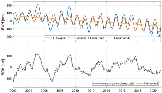
Figure 1.
Example for the decomposition of a mTWS time series into linear trend, seasonal, subseasonal and interannual signal. The location is 13 °E and 52.5 °N (Potsdam, Germany), the model is GFDL-CM4 (r1i1p1f1 run).
The decomposition is performed for each land grid cell, for each of the 105 CMIP6 ensemble members, for the unscaled MMMed model time series, and for the GRACE data set. Furthermore, it is applied on two different time spans, 2002/04–2020/04 (the GRACE and GRACE-FO period) and 2000/01–2100/01 (only for the model data). To ensure consistency for the comparison between GRACE and models, the 11 month data gap between GRACE and GRACE-FO was also excluded from the model time series prior to decomposition. As information on the accuracy of the grid values for the GRACE and the unscaled MMMed model time series is available, we can strictly propagate these during the parameter estimation in Equation (5), ending up with standard deviations , ..., for the different signal components for each grid cell. For the 105 individual model runs we have no information on their accuracy, hence, no error estimates for their signal components, so that only the ensemble spread is used to characterize model uncertainty.
2.4. Relative Importance of Signal Components
We now split TWS and mTWS signals into different temporal components as described above. For each signal part in each grid cell, we compute the signal variance over the GRACE time span and relate it to the variance of the total signal. The fractional variance composition for the long-term, seasonal and sub-seasonal signal is displayed in Figure 2. The colors in Figure 2 are assigned by mixing the red, green, and blue (RGB) color values according to the fractions of the variance components, meaning that pure blue would indicate a perfect seasonal signal with no long-term or sub-seasonal components. Pure green characterizes no seasonal or sub-seasonal variations, and pure red a location with only sub-seasonal variability. A signal with equal long-term, seasonal and sub-seasonal variance would be displayed white, and other mixtures with the colors in-between. The variance component analysis of the GRACE TWS time series (Figure 2a) reveals that many regions at moderate latitudes are particularly affected by long-term variations, so that water availability as represented by TWS is particularly modified from long-term natural (or anthropogenic) climate variability.
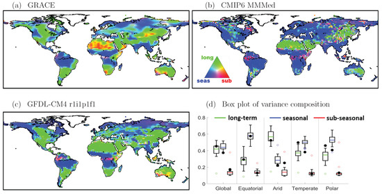
Figure 2.
Distribution of the total variance into long-term, seasonal and sub-seasonal variability for the time span 2002/04–2020/04 for (a) the GRACE TWS observations, (b) the MMMed of the simulated mTWS, (c) an exemplary individual model run (GFDL-CM4 r1i1p1f1). (d) Box plot of the variance composition within the model ensemble for the global average and averaged over different climate zones. Black dots denote the respective result for the GRACE observations.
Repeating the same variance component analysis for the unscaled MMMed mTWS time series of the 17 models instead results in a pattern largely dominated by the seasonal variance (Figure 2b), which is very distinct from the results obtained from GRACE. This discrepancy reveals a caveat of using the unscaled MMMed for comparison with observations: Climate models are able to represent interannual and sub-seasonal TWS variations in a statistical manner only. This implies that the exact timing of the occurrence of troughs and peaks in the time series is random so that model runs and observations are not directly comparable on time series level in terms of, e.g., correlation or RMSD. Hence, time series of interannual and sub-seasonal TWS variations from different model runs can match only regarding their magnitude and frequency, but not at specific points in time. Therefore, when building the model average, the interannual and sub-seasonal variabilities that are contained in the individual model runs are not maintained but largely smoothed out. As a consequence, mainly seasonal signals remain in the MMMed. Thus, it is not feasible to directly compare the signal variability of the unscaled MMMed time series with the observations, but we have to revert to investigating the variability of individual ensemble members.
Exemplarily, in Figure 2c the variance composition of one specific run (r1i1p1f1) of the GFDL-CM4 is shown, which exhibits much more similarities with the observational pattern in Figure 2a than the unscaled MMMed pattern. Hence, for the remaining sections of the paper, we first perform the signal decomposition for all 105 ensemble members and afterward calculate the MMMed and its respective standard deviation for the individual components (e.g., annual amplitude) according to Equations (2) and (3).
To achieve a comprehensive overview over the variance composition in the whole model ensemble, we aggregate the fractional variance components as follows: For each of the 105 ensemble members we compute for each land grid cell the variance composition (as before: three fractional values for long-term, seasonal, and sub-seasonal, adding up to 1.0). Afterward, we compute for each ensemble member the global land average of the individual component fractions, resulting in 105 times 3 values representing the model range of variance compositions for the global mean. This range of variance compositions is displayed in the left of Figure 2d. The boxes represent the median (colored line), the 25% and 75% percentile (bottom and top edge of box) and the most extreme data points not considered outliers (whiskers) in the data set of ensemble members. The outliers are displayed separately with colored circles. For comparison we also compute the global land average for the three variance components of the GRACE record (black dots in Figure 2d). Furthermore, we repeat the averaging of the component fractions for different Köppen-Geiger climate zones [35] (further diagrams in Figure 2d). Please note that in all global (and regional) land averages provided in this study, Greenland and Antarctica are excluded from the computations as mass change in these regions is dominated by ice mass variations, which are not represented by the ESMs. Comparing the model results to the observations (Figure 2d) we note that for the fractional long-term component the models are close to GRACE in equatorial and arid regions but underestimate it in temperate and polar regions. The fraction of the annual cycle, however, is mostly overestimated by the models except for equatorial regions. The fit of the sub-seasonal variance fraction is good for equatorial, temperate and polar regions. In arid regions the sub-seasonal variance fraction in the models is smaller than in the GRACE observations. One reason for this is probably inherent noise in the gravity data causing a low signal-to-noise ratio in arid regions with low signal variability. In equatorial regions the variance composition into long-term, seasonal and sub-seasonal signal fits remarkably well to the observations, whereas it is more discordant in the other regions.
2.5. Building and Rescaling the MMMed for Measures of Variability
In the previous section we pointed out that the computation of an unscaled MMMed grid time series from all 105 ensemble members results in a reduced interannual and sub-seasonal variability. Thus, to analyze the variability in the model ensemble, we separately decompose all 105 ensemble member time series and define the amplitude and phase of the annual cycle as well as the Root Mean Square (RMS) of the interannual signal component as the measures of signal variability to be investigated. Only afterward we then compute the MMMed grid over these measures. By this, we maintain the overall variability of the model ensemble and obtain for each signal variability measure a global pattern reflecting the best estimate for its spatial distribution.
However, there is a second issue arising from building an unscaled MMMed on grid cell level: as the global patterns differ for different model runs, the median smooths out extreme values in each grid cell. Thus, the range of values in the unscaled MMMed grid is much smaller than the actual range of values in the individual ensemble members (and the observations). For illustration, Figure 3 displays the empirical cumulative density functions (ECDFs) for the 5–95% percentiles calculated from the land grid cells of all model runs for one of the measures we investigate (interannual RMS change, Section 3.2.2). Additionally, the ECDF of the unscaled MMMed is shown (thick red line), which has a much smaller range and thus cannot be regarded as a realistic representative for the variability. Thus, we adjust the range of values in the MMMed as follows: we compute the weighted multi-model median of all 105 ECDFs (thick black line in Figure 3) to obtain a best estimate for the range of simulated values, and divide it for each percentile by the ECDF value of the unscaled MMMed (thick red line). Each grid cell value of the unscaled MMMed map is then multiplied with the factor belonging to its respective percentile. As a result, the ECDF of the scaled MMMed equals the MMMed of the 105 ECDFs of the ensemble members (thick black line). Consequently, also the scaled MMMed standard deviation is adjusted by this factor. The scaling of the MMMed ensures that not only the global pattern but also the range of values states a representative estimate of the model results. Thus, in the rest of the paper, all comparisons (as far as referring to a model average) are performed with respect to the scaled MMMed. If only MMMed is written, it always means the scaled MMMed.
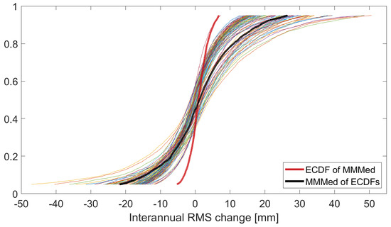
Figure 3.
Example for different range of values for the ensemble members and the MMMed.
3. Results
In Section 3.1 we compare the CMIP6 mTWS model results to GRACE TWS observations for the time span 2002/04–2020/04 in terms of annual cycle (amplitude and phase) and interannual variations as derived from the signal decomposition. From the models the (scaled) MMMed as a best estimate for the respective signal component is used in the comparison. Afterward, in Section 3.2 the future development of the annual cycle and interannual variations for the time span 2000/01–2100/12 is assessed by the MMMed (serving as expectation value) of the respective signal component changes. Furthermore, the MMMed long-term linear trend is evaluated. We also discuss the consensus of the models on the projected changes. In Section 3.3, in order to provide a first hint about the detectability of projected TWS annual cycle changes, the MMMed annual cycle changes over 30 years are compared to the accuracy of GRACE and possible NGGM observations. In the last part (Section 3.4) we select a specific model run from the ensemble of 105 members that can serve as input for NGGM simulation studies. In this selection process, we consider both the fit of the model run to GRACE observations in the GRACE time span (for annual cycle and interannual variations) and to the MMMed in the projected time span (for changes in amplitude, phase, interannual variations, and linear trends). An overview of the different evaluation time spans and measures discussed in this section is given in Table 1.

Table 1.
Overview over the different signal components analyzed for different time spans.
3.1. Current TWS Variability in CMIP6 Models and GRACE
3.1.1. Seasonal Cycle
Here we compare GRACE and CMIP6 models first regarding the annual amplitude. The global patterns (parameter c of Equation (5)) from GRACE and the (scaled) MMMed annual amplitudes from 17 CMIP6 models (Figure 4a,b) are visually similar and feature a pattern correlation of 74%. The pattern correlation of two grids is calculated by arranging (for each grid separately) the values of all land grid cells into a vector and computing the Pearson product-moment correlation coefficient of the two vectors. The correlation coefficient can be regarded as a measure of pattern similarity for the two grids.
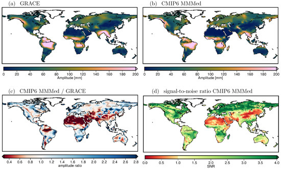
Figure 4.
(a) GRACE TWS annual amplitude and (b) scaled MMMed mTWS annual amplitude for the time span 2002/04–2020/04. (c) Ratio of (b) and (a). Stippling indicates regions where the deviation from 1 exceeds the standard deviation of the ratio. (d) MMMed mTWS annual amplitude signal-to-noise ratio.
To compare the model results and GRACE, we compute the ratio between the CMIP6 MMMed amplitudes and the GRACE amplitudes (Figure 4c). The more the ratio differs from 1 in a certain grid cell, the less the amplitudes from models and GRACE correspond in this grid cell. To objectively rate the magnitude of the deviation, the uncertainty of the ratio has to be considered. The standard deviation of the ratio is derived from the model spread of the MMMed amplitude (Equation (3)) and the standard deviation of the GRACE amplitude via variance propagation. We find that for 66% of the global land area (without Greenland and Antarctica) the amplitude ratio deviations from 1 lie within the standard deviation of the ratio. Large parts of the deviations that exceed the error bounds (stippled regions in Figure 4c) are located in arid regions of Northern Africa and the Arabian Peninsula, which generally exhibit a small annual cycle of TWS, and thus the relative uncertainties are larger. To facilitate a more detailed analysis of the CMIP6 amplitudes and their relation to GRACE we calculate the CMIP6 signal-to-noise ratio (SNR) for the annual amplitude (MMMed amplitude divided by the model spread of the MMMed amplitude, Figure 4d). Apart from regions with very small values (discussed below) the SNR is generally higher in the northern hemisphere than in the southern hemisphere. We attribute this to the fact that for many observational records (especially in situ observations) the coverage in the northern hemisphere is denser and thus the calibration of existing climate models is askew respectively, leading to a reduced model spread for northern regions.
In the arid regions of Northern Africa, the Arabian Peninsula, and in large parts of China and Mongolia, the SNR is very small or even below 1. In these regions, the annual cycle is generally not very distinctive (Figure 4b), as can also be seen from the composition map in Figure 2c: the dominating component of the time series in the regions of small SNR is the long-term or sub-seasonal signal. Thus, meaningful results for the annual cycle cannot be expected in these regions. We decided to exclude regions with a SNR of the CMIP6 amplitudes below 1 (24% of the global land area) prior to a regional analysis of the amplitude deviations between CMIP6 and GRACE, because otherwise the statistical measures would be largely distorted.
While putting regions with SNR below 1 aside, the median overestimation of the amplitude with respect to GRACE (area-weighted median of all ratios in Figure 4c above 1) is 1.38 and the median underestimation (area-weighted median of all ratios below 1) is 0.79. The land area where the annual amplitudes are overestimated by the models is larger than the area where it is underestimated (58% vs. 42%). This proportion varies depending on the climate zone. For the regional analysis we access the Köppen-Geiger climate classification [35] and compute the median over- and underestimation for four different regions characterized by arid, equatorial, temperate, and polar climates. All numbers of the regional analysis are given in the Supplementary Material (Tables S1–S7). The regions with SNR below 1 are mainly arid: here, 50% of the area is excluded, whereas in the other climate regions this fraction is only 10%. The proportion of overestimation to underestimation in equatorial regions is 51% to 49%, i.e., a more even proportion compared to the global values. In contrast, the annual amplitude is mainly overestimated (65%) in polar regions. A tendency of underestimation in tropical regions and overestimation in northern regions was also found by Scanlon et al. [34] for a selection of hydrological models and land surface models, especially for the CLM-5.0 model that is the land surface component in two ESMs investigated in this study (CESM2-WACCM, NorESM2-LM). Particularly large amplitude underestimation of CMIP6 amplitudes compared to GRACE that exceeds the model uncertainty occur in the Amazon and the Ganges-Brahmaputra basin. We suppose that the water holding capacity is bound-limited in models, leading to an overly strong runoff of excess water. In addition, soil moisture memory is often too short in models especially in equatorial regions, preventing the accumulation of water to its real storage extent. The overestimation of the amplitude by the models in the north might be related to overestimated snow storage in winter and evapotranspiration in summer, thereby simulating an overall increased annual amplitude [34].
In addition to the amplitude we also investigate the MMMed phase of the annual cycle (i.e., the month of the annual TWS maximum, derived from parameter d of Equation (5)) and compare it to the GRACE-derived phase (Figure 5a,b). Please note that phase values are cyclic and cannot be assumed to be normally distributed. A scheme for the calculation of a weighted median from phases and its standard deviation is described in the Supplementary Material (Section S5). As the computation of a ratio of phases between models and GRACE is not feasible, we only calculate the differences between the MMMed phases and the GRACE phases (Figure 5c) to compare the two grids. The accuracy of the phase differences is computed by error propagating the model spread of the MMMed phase and the standard deviation of the GRACE phase. In 74% of the global land area the differences between the GRACE and the model phases do not exceed the standard deviation of the difference (Figure 5c).
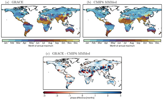
Figure 5.
(a) GRACE TWS month of the maximum of the annual cycle and (b) MMMed mTWS month of the maximum of the annual cycle for the time span 2002/04–2020/04. (c) Difference of (a,b). Stippling indicates regions where the difference exceeds the standard deviation of the difference.
Particularly large differences occur in the arid regions of Northern Africa and the Arabian Peninsula, as well as in those parts of China and Mongolia that exhibit a very small SNR of the amplitude (Figure 4d), hence a weak annual cycle that prevents meaningful phase estimates. Therefore, we again exclude regions with an amplitude SNR below 1 from the further analysis. The remaining differences are mainly positive (72% of land area), meaning that the observed annual cycle is slightly lagged behind the modeled cycle. The median positive phase shift (models earlier, 72%) is 0.50 months, and the median negative phase shift (models later, 28%) is −0.32 months. The mainly positive phase shift between observations and models might be related to missing groundwater processes in CMIP6 models causing an underestimation of the water residence time in the soil, hence less time for storage accumulation and consequently an earlier saturation of the maximum storage. The tendency of the models to precede the observed annual cycle was also found for the hydrological and land surface models investigated by Scanlon et al. [34]. It is larger in the polar climate zone (82%) than in the equatorial zone (62%).
3.1.2. Interannual Anomalies
In several parts of the world long-term variations (linear trends plus interannual variations) in TWS are the dominating part of the signal variability (Figure 2). The direct comparison of linear TWS trends from GRACE and ESMs is difficult because the models do not include all physical processes (e.g., surface water, glacier, and anthropogenic groundwater change) that contribute to observed TWS, and therefore are not able to fully represent long-term trends everywhere. Furthermore, over a time span of less than 20 years trends are largely influenced by interannual variability [13], so that we focus on interannual variations only. As elaborated in Section 2.3, model time series of interannual variations are not directly comparable due to the random occurence of such variations in the models. Therefore, we chose the RMS of the interannual variability over 2002–2020 as a measure for comparison. Similarity of the RMS between models and GRACE over a 18-year time span would prove that the models are able to capture the general range of observed interannual variability independent of the exact evolution of the time series. Indeed, the global patterns of the GRACE interannual RMS and the MMMed interannual RMS (Figure 6a,b) feature similarities in many regions of the world. The global pattern correlation for the MMMed with GRACE is 64%, which is lower than the correlation for the annual amplitude, but nearly as high as the correlation of the MMMed with its individual model ensemble members (), which highlights the large intermodel spread of the interannual TWS variability in ESMs.
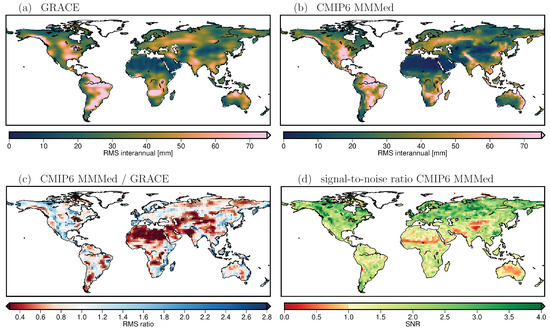
Figure 6.
(a) GRACE TWS interannual RMS and (b) MMMed mTWS interannual RMS for the time span 2002/04–2020/04. (c) Ratio of (b) and (a). Stippling indicates regions where the deviation from 1 exceeds the standard deviation of the ratio. (d) MMMed mTWS interannual RMS signal-to-noise ratio.
As we did when analyzing the annual amplitude, we also compute the ratio of the MMMed interannual RMS and the GRACE interannual RMS (Figure 6c). As before, the accuracy of the ratio is derived by variance propagation of the respective MMMed and GRACE accuracies. Regions, where the deviation of the ratio from 1 exceeds its standard deviation, correspond to 31% of the land area (stippling in Figure 6c), mainly in South America, Central and South East Asia, and in large parts of Africa. The interannual RMS is underestimated compared to GRACE observations in 60% (regions of SNR < 1 from Figure 6d excluded) of the global land area. This proportion is relatively constant for the different climate zones (54% to 68%). There are also regions where the interannual RMS in models is overestimated compared to GRACE (40%), mainly in coastal areas (North and West Europe, Australia, East Coast of Africa, North Coast of Canada) and in the mountainous areas in North America. It would be interesting to explore reasons for those discrepancies in cooperation with climate scientists that are developing the CMIP6 models. The model signal-to-noise ratio, i.e., the MMMed interannual RMS divided by its standard deviation (Figure 6d), is generally smaller than for the annual amplitude, which confirms that the representation of the seasonal cycle in ESMs is more reliable than the representation of interannual variations. This is an expected result as the underlying physical processes driving interannual fluctuations are more complex and less known than the annual cycle, causing its modeling to be more challenging.
3.2. Projected Change in TWS Variability until 2100
Model projections until 2100 provide valuable information about the future development of TWS. We therefore analyze changes in the annual cycle and interannual variations of the CMIP6 mTWS signal for the time span 2000/01–2100/12. Additionally, we analyze the long-term linear mTWS trend. The analysis is done for the (scaled) MMMed taken as expectation value for the future development of the climate.
3.2.1. Seasonal Cycle Changes
Centennial changes in the annual mTWS amplitude are obtained by accessing parameter in Equation (5) from the model signal decomposition over 2000/01–2100/12. The (scaled) MMMed of the amplitude changes exhibits values on the order of several mm EWH per decade (from −2.75 mm/yr to 1.83 mm/yr, with a median absolute value of 0.11 mm/yr), which are substantially varying locally (Figure 7).
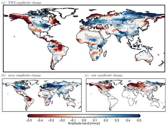
Figure 7.
(a) MMMed mTWS annual amplitude change over 2000–2100. Stippling indicates regions where 13 or more of 17 models (i.e., ≥76%) agree on the sign of the amplitude change. (b,c) same as (a) but for mrso and snw.
In 45% of the land surface more than three quarters of the models (13 or more of 17, ≥) agree on the direction of the amplitude change. These regions are stippled in Figure 7 and are referred to as high consensus regions in the following. As in high consensus regions many models are concordant about the direction of the change we consider the results in these regions as particularly reliable. In many regions a high model consensus corresponds to a large magnitude of the amplitude change (e.g., in Europe and Northeast Asia, Canada) and analogously low consensus goes along with small changes. However, there are exceptions from this rule. For example, there is only low model consensus about changes in amplitudes in large parts of South America although the mean amplitude changes especially in the Amazon basin are among the largest signals. Also in Central Africa the decreasing amplitude is not supported by high consensus. Conversely, there are also regions of small amplitude changes but high model consensus. These often also feature a small seasonal cycle, e.g., in Northern Africa and in Central Asia.
According to the models, in the majority of the land area (56%) the seasonal amplitude will increase until 2100, with a median of 0.12 mm/yr. The median of the amplitude decrease (44% of the land area) is −0.11 mm/yr. The area proportion of positive to negative changes is even more pronounced when restricting to high consensus regions (66% increasing amplitude with median 0.21 mm/yr, 34% decreasing amplitude with median −0.26 mm/yr). Furthermore, the distribution of amplitude changes depends on the climate zone, e.g., the proportion of increasing vs. decreasing amplitudes is more balanced in the equatorial zone (51% vs. 49%), and more distinct in the polar zone (69% vs. 31%) compared to the global distribution. The relatively strong amplitude increase in polar regions (median of 0.18 mm/yr) originates mainly from the soil moisture component of the ESMs, as can be seen from Figure 7b,c that show the amplitude changes for the mrso and snw variable separately. In the snow component a decrease in the annual amplitude is projected with high consensus, which is related to generally rising temperatures and reduced snow accumulation until 2100. The increase of the soil moisture amplitude might be due to increased evapotranspiration in a warmer climate therefore reducing water storage during summer.
Together with the linear trend of the annual amplitude we also estimate for each grid cell (and for each ensemble member) a linear trend of the phase of the annual cycle (parameter in Equation (5)). These linear trends can be converted to a MMMed total phase shift from 2000 to 2100 (Figure 8).
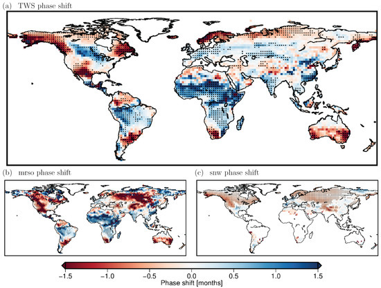
Figure 8.
(a) MMMed mTWS phase shift of the annual cycle over 2000–2100. Stippling indicates regions where 13 or more of 17 models (i.e., ≥) agree on the sign of the amplitude change. (b,c) same as (a) but for mrso and snw.
In 37% of the land surface more than three quarters of the models (13 or more out of 17) agree on the direction of the phase shift. For the majority of the land area (55%) the models project a positive phase shift, i.e., the maximum of the annual cycle is reached later in 2100 than in 2000 (median of 0.39 months, approx. 12 days). The median of the 45% land area where the maximum is reached earlier is −0.35 months (approx. 11 days). The tendency to a later annual cycle is particularly strong in the equatorial zone (75% later, with a median of 0.49 months). Especially in Africa large parts of the continent will experience a substantial later peak of the annual TWS maximum according to a majority of the models. This is related to a later onset of the rainy season which was identified already in CMIP5 models by Dunning et al. [36] who attribute this to a position shift in the tropical rain belt and increasing strength of the Saharan heat low.
In the polar climate zone the area proportion of positive and negative phase shifts is opposite to the global (only 41% later and 59% earlier). We relate this to a generally shorter accumulation period of snow and an earlier onset of thawing due to higher air temperatures. When splitting the mTWS signal into the soil moisture and the snow component (Figure 8b,c) it is striking that in large parts of the polar climate zone both the mrso and the snw MMMed exhibit a strong negative phase shift (earlier reach of maximum in 2100), whereas the sum of both (mTWS MMMed) has a small positive phase shift. This is a result of the interference between the mrso and snw signals which mostly show growing mrso amplitudes and shrinking snw amplitudes in polar regions (compare Figure 7b,c) and are shifted in their respective phases. An example for this effect is given in the Supplementary Material (Section S6). This finding highlights the importance of an accurate modeling of all individual TWS components and their relative magnitude and phase, thereby underscoring once more the importance of satellite-based surface mass observations for guiding the numerical modeling of the global water cycle.
3.2.2. Interannual Anomaly Changes
Changes of the RMS of the interannual signal over 2000–2100 were identified by computing the MMMed of the differences between the interannual RMS over two time spans, one at the end (2082–2100) and one at the beginning (2002–2020) of the investigated time period (Figure 9).
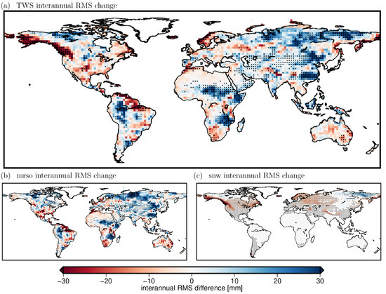
Figure 9.
(a) MMMed mTWS interannual RMS change from 2002–2020 to 2082–2100. Stippling indicates regions where 13 or more of 17 models (i.e., ≥) agree on the sign of the RMS change. (b,c) same as (a) but for mrso and snw.
A slight increase of interannual variability is projected by the models for the majority of the land area (54%) with a median value of 7.02 mm. The median negative RMS difference is −5.75 mm (in 45% of the land area). However, the general pattern of the MMMed interannual RMS change is not as distinct as it is for changes in the annual cycle (Section 3.2.1), and in only 23% of the land surface a high model consensus (≥) is found. This is probably related to the larger intermodel spread for interannual variations compared to the seasonal signal (cf. Section 3.1.2). The proportion of land area with positive vs. negative RMS changes is quite similar for all climate zones (between 50% and 57% positive), thus no clear regional dependence of the development for interannual variations can be identified. However, when splitting the mTWS signal into its components soil moisture and snow (Figure 9b,c) a clear decrease of the snow interannual variability (supported by more than three quarters of the models) is found for all snow covered regions (except for a small patch in North East Siberia), whereas the polar zone in the soil moisture projection is largely dominated by an increase of interannual variability.
3.2.3. Long-Term Trends
In addition to changes in the annual cycle and interannual variations, the long-term linear trend affects the possible range of future TWS. Centennial mTWS trends in coupled climate models and their relation to GRACE were investigated in Jensen et al. [13] for CMIP5, and we thus give a short update on the findings for CMIP6. The centennial median mTWS linear trend (parameter b in Equation (5)) from each 17 CMIP6 and CMIP5 models is shown in Figure 10. As before, stippling indicates regions of high consensus (≥13 of 17 models agree in sign).
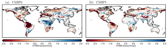
Figure 10.
(a) MMMed mTWS linear trend over 2000–2100. Stippling indicates regions where 13 or more of 17 models (i.e., ≥) agree on the sign of the trend. (b) same as (a) but for 17 CMIP5 models.
The model consensus among the CMIP6 models is substantially higher than for the CMIP5 models. For CMIP6, in 47% (27% drying, 20% wetting) of the land area more than 76% of the models agree on the trend sign for CMIP6, whereas this number is only 35% (21% drying, 14% wetting) for CMIP5. Especially in Central Africa, South America and Russia/Central Asia the regions of consensus grow from CMIP5 to CMIP6. Furthermore, the median positive and negative trends (0.42 mm/yr and −0.42 mm/yr) are larger for CMIP6 than for CMIP5 (0.18 mm/yr and −0.36 mm/yr). The trend pattern is similar, but it intensifies from CMIP5 to CMIP6 in many regions, e.g., in Central Africa (more intense wetting), tropical South America, and the Mediterranean Coast (more intense drying). In Jensen et al. [13] and Scanlon et al. [37] a general underestimation of the magnitude of linear mTWS trends compared to observations was found. Hence, we conclude that representation of trends improved with the new model generation.
Conclusions on the reliability of centennial linear trends in ESMs are difficult to draw, as the ability of models in representing current trends cannot be verified by observations yet due to the length of the record. Interannual variability largely superimposes possible long-term trends in time spans of less than 30 years, and thus trends over shorter periods are not directly comparable for observations and models [13]. Even if a sufficiently long observational record was available, in some regions trends from observations and models would still not be comparable due to missing processes and components in the models (e.g., groundwater processes, surface water dynamics, anthropogenic contributions).
3.3. Detectability of Annual Cycle Changes
Model analysis in Section 3.2.1 and Section 3.2.2 revealed that significant long-term changes of TWS variability are to be expected, likely with implications on the future water cycle. Now we investigate to which extent changes as projected with CMIP6 models will be detectable with gravity missions such as GRACE/GRACE-FO or a NGGM. For a first assessment, we assume an observation period of 30 years and restrict the analysis to changes of the annual cycle (amplitude and phase). We consider a signal (i.e., an amplitude or phase change) to be detectable if it exceeds the accuracy of the respective observations. The signal, i.e., the absolute amplitude change for 30 years, is obtained by multiplying the MMMed amplitude change pattern (Figure 7a, given in mm/yr) by 30 years. The absolute phase change for 30 years is derived by scaling the MMMed phase change pattern (Figure 8a; given as absolute change over 100 years) with 0.3 (for 30 years). We then compute accuracies for these absolute 30-yr amplitude and phase changes for two cases, assuming (1) the current GRACE accuracy and (2) a possible NGGM accuracy being 5 times better than for GRACE. This accuracy is proposed as a minimum target performance for NGGMs and is supposed to be achieved by, e.g., employing multiple satellite pairs (double-pair mission), a more favorable orbit design, and improved instrumentation regarding accelerometers and inter-satellite ranging [18,38]. The amplitude and phase change accuracies for cases (1) and (2) are both taken from the accuracies of parameters and of Equation (5) as described in Section 2.3 under the assumption of a 30 year long time series.
The resulting absolute amplitude and phase change standard deviations (Figure 11a,b) are compared to the absolute amplitude and phase change patterns. In grid cells where the magnitude of the latter exceeds the former the signal is considered to be detectable after 30 years of observations. With a system maintaining the current accuracy of the GRACE mission, and supposing a change pattern as predicted by the MMMed of the 17 CMIP6 models, amplitude changes will be detectable after 30 years in 34% of the land area, and phase changes in 28% of the land area (Figure 11c,d). The threshold for a change being detectable varies spatially as the accuracy pattern is not uniform due to the GRACE error structure. Assuming a NGGM accuracy outperforming the GRACE accuracy by a factor of five but maintaining the same TWS error pattern, amplitude changes would be detectable in 75%, and phase changes in 66% of the land area (Figure 11e,f). Only in very dry regions possible tiny changes in the practically non-existent annual TWS cycle would not be detectable with such a NGGM mission, implying that such changes could be detected reliably everywhere on the continents where agricultural activities take place.
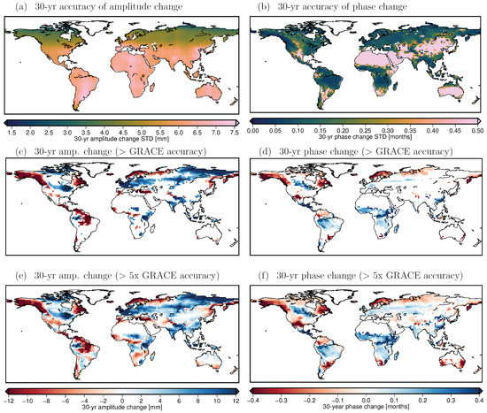
Figure 11.
(a) standard deviation of GRACE TWS annual amplitude change over 30 years. (b) standard deviation of GRACE TWS phase change of annual cycle over 30 years. (c) MMMed mTWS annual amplitude change over 30 years that exceeds the GRACE accuracy (given in (a)). (d) same as (c) but for phase change. (e,f) same as (c,d) but assuming the standard deviation of GRACE (given in (a,b)) being five times smaller.
3.4. Selection of a Representative Model Run for NGGM Simulations
Important prerequisites for the implementation of a NGGM are on the one hand the demonstration of user needs, and on the other hand the justification of science return and societal benefit of a proposed mission concept. Therefore, numerical full-scale simulations are of utmost importance to quantify the achievable performance of an NGGM, and to demonstrate that the science requirements can be met by a certain mission concept and instrumentation. The need for sustained observation of mass transport from space was expressed by an international expert panel under the umbrella of IUGG representing all relevant geoscientific applications [18], and amplified by a resolution adopted by the Council of the International Union of Geodesy and Geophysics [39]. Several numerical simulation studies showed the added value of double-pair concepts for hydrological applications (e.g., [40], and references therein). The main outcome of these numerical simulations is the rating of achievable performance of a mission concept regarding accuracy, spatial and temporal resolution, against the characteristics of the target TWS signal. Up to now, mainly the short-term behaviour of NGGM concepts was evaluated, but hardly any long-term simulation studies focussing on interannual variations and trend signals exist. An exception might be the NGGM study on earthquake detectability by [41], where a mission lifetime of 12 years was simulated to capture full earthquake cycles. For a realistic assessment of the achievable performance over long time periods, it is not sufficient to simply propagate the errors obtained from a short-term simulation to a longer time span. Full-fledged long-term simulations are needed because (1) the relative error contribution of instrument errors and temporal aliasing errors to the total error budget significantly changes with increasing averaging period, (2) they enable a direct parametrization of (linear or non-linear) trends thereby providing a more robust estimate, and (3) they allow for the co-estimation of ocean tides and separation of tidal constituents with very similar excitation periods. While the assessment of the achievable long-term mission performance of potential NGGMs together with an adequate uncertainty characterization is beyond the scope of this study, such simulations need input information on mass changes. Especially for the investigation of climate-driven effects, realistic time series of a possible future development of TWS as input for long-term satellite simulations are of great importance.
In the previous sections the TWS variability was discussed for the (scaled) multi-model median as a best estimate from 17 CMIP6 models with 105 ensemble members in total. However, as elaborated in Section 2.3, the TWS time series of a MMMed is not suitable as input for a NGGM simulation study because the interannual and sub-seasonal variability in the individual model runs is not maintained in the MMMed but largely averaged out. Consequently, for a NGGM simulation study input, a specific model run from the 105 ensemble members has to be selected. Ideally, such a specific model run should be (1) similar to the observations during the GRACE time span, and (2) representative for the expected changes until 2100. This means that for (1) we compare the annual cycle and interannual RMS maps of all 105 ensemble members to the GRACE annual cycle and interannual RMS maps. For (2), we relate the amplitude, phase, and interannual RMS change maps as well as the long-term linear trend maps of the 105 ensemble members to the respective maps of MMMed, which are our best guesses for future TWS variability changes. We recall that MMMed maps are calculated by first decomposing all ensemble members separately and then computing the MMMed for each measure which is different from the decomposition of the MMMed mTWS time series. For the identification of a representative model run we consider two measures to judge similarity between two grids: (a) the pattern correlation to account for the spatial pattern and (b) the RMSD of the empirical cumulative distribution functions (ECDFs) to account for the range of values. During computation of (a) and (b) for the annual cycle we switched from the amplitude and phase representation to coefficients for in-phase and quadrature phase components. This transformation is necessary since only the latter can be assumed to be normally distributed so that conventional statistical metrics can be readily applied. As a result from calculating (a) and (b), for each ensemble member we obtain 14 numbers describing the similarity of the model run with the GRACE observations and with the MMMed: the pattern correlation (a) and ECDF RMSD (b) for (1) sine amplitude, cosine amplitude, and interannual RMS compared to GRACE, and (2) for amplitude change, phase change, interannual RMS change, and linear trend compared to the MMMed.
After computing the 14 metrices for all 105 ensemble members, we perform a ranking: For each metric its range of values is distributed into 100 equidistant classes and dependent on the class into which the respective value of a ensemble member falls, a rank is assigned (1 = smallest rank, smallest similarity; 100 = highest rank, highest similarity). Please note that for the RMSDs of the ECDFs we take the negative values for ranking in order to maintain the rating of the classes (high for good match and low for poor match). Afterward, the ensemble members are sorted with descending mean rank over the 14 metrices. The ranking reveals that no single model run is clearly superior to all others. Instead, model runs of the GFDL-CM4, EC-Earth3, MIRCO6, and CanESM5 exhibit a similar mean performance (Figure 12). Furthermore, the high-ranked model runs do not in every case perform best for all metrices. E.g., the pattern correlation of the annual cycle from most of the top-ranked models with the GRACE annual cycle (first and third column in Figure 12) is only ranked medium high and does not differ substantially from many low-ranked models. On the other hand, an overall low-ranked model does not necessarily occupy poor ranks in all metrices. We note that the rank classification is relative to the range of values of the respective metric but not to its distribution. This means that it is sensitive to outliers: for example, one single model run with an extraordinary high similarity and all others lower (but homogeneous) would lead to the assignment of the first rank to the earlier and the last rank to all later, regardless if the absolute value of the similarity for the other ensemble members may still be pretty good. Thus, in the ranking we do not rate the absolute goodness of similarity but only the performance of the model runs with respect to the others within a specific metric. The full table with the ranking for all 105 ensemble members is given in the Supplementary Material (Figure S6).
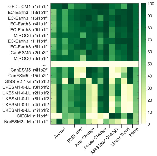
Figure 12.
Ranking of the ensemble members according to the classes assigned with pattern correlation (odd columns) and RMSD of ECDF (even columns) of annual cycle and interannual RMS with GRACE (colums 1–6) and amplitude change, phase change, interannual RMS change and linear trend with the MMMed (columds 7–14). Mean rank given in column 15. The upper 10 ensemble members are the best performing, the lower 10 the worst. The full ranking table is provided in the Supplementary Material, Figure S6.
According to the ranking, the model run GFDL-CM4 ri1p1f1 has the best mean match with GRACE and the MMMed on the basis of our selected metrices and rating strategy. Thus, this model run can be considered to be a representative model run of the ensemble regarding its similarity to observations and its alignment with the MMMed and can serve as input for NGGM simulation studies. The mTWS variability in the GFDL-CM4 r1i1p1f1 in terms of annual cycle and interannual variability (with their projected changes) and the long-term linear trend is given in Figure 13. In the Supplementary Materials (Section S8) we provide the results for the detectability of GFDL-CM4 ri1p1f1 annual cycle changes with the GRACE mission or a potential NGGM as described in Section 3.3.
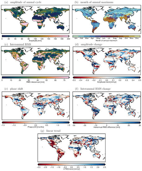
Figure 13.
mTWS variability of selected model run GFDL-CM4 r1i1p1f1. (a) Amplitude of annual cycle, (b) month of the maximum of the annual cycle, (c) interannual RMS; (a–c) for the time span 2002/04–2020/04. (d) change of the annual amplitude over 2000–2100, (e) phase shift of the annual cycle over 2000–2100, (f) interannual RMS change from 2002–2020 to 2082–2100, (g) linear trend over 2000–2100.
4. Conclusions
Based on the CMIP6 multi-model ensemble, we assess the current variability of TWS with respect to the observational record acquired by the GRACE and GRACE-FO satellite missions in the time span 2002/04–2020/04 and investigate potential changes in that variability that can be expected to happen until the end of the present century under increasingly changing climate conditions.
In a first step, we compared the general composition of the variances from the seasonal, long-term and sub-seasonal TWS signal in CMIP6 models to the observed signal variances, concluding that the model ensemble represents the current climate conditions reasonably well. While globally the models have a tendency to overestimate the seasonal cycle component and to slightly underestimate the sub-seasonal and long-term signal variance, in equatorial regions we report an overall remarkably good match of all variance components.
To further investigate the fit of different TWS signal components from models and observations we compared the CMIP6 MMMed maps of the annual cycle (amplitude and phase) and the RMS of the interannual signal to the respective GRACE-derived maps. For the annual amplitude the global patterns are similar, with an underestimation by the models in the equatorial climate zone, and an overestimation in the polar zone. Furthermore, the fit is degraded in regions with a small model signal-to-noise-ratio (SNR), mainly in regions with an insignificant annual cycle. For the phase of the annual cycle we found that the models precede the GRACE observations in the majority of the land area (72%) by about half a month in average. We attribute this to missing groundwater processes in CMIP6 models causing an earlier reach of maximum storage due to reduced soil water residence times. The positive time lag of the observations is more pronounced in polar regions than in the other climate zones. For the RMS of the interannual signal the similarities with observations are not as strong as for the annual cycle, and the intermodel spread is larger. As expected from the analysis of the variance components land areas where models underestimate the interannual signal regarding GRACE (60%) exceed areas of overestimation.
In addition to the present-time match of modeled and observed TWS variability, it is important to analyze future changes of TWS variability until 2100. Such information can be useful to refine user requirements for NGGMs that can be readily applied in satellite simulation studies. According to the CMIP6 models, changes in the annual amplitude of regionally up to 27 mm per decade are to be expected. In many regions (45% of the global land area) more than 76% of the models show the same direction of the amplitude change, which is positive in the majority of the land area (56%). The models are less concordant about phase shifts of the annual cycle. In 37% of the land area 76% or more of the models agree on the direction of the shift. A particularly strong phase shift was found for equatorial regions, where until 2100 in 75% of the area the maximum of the annual cycle is projected to be reached on average over two weeks later. The model consensus on changes of the interannual signal is still smaller than for the phase shifts; only in 23% of the land area more than 76% of the models agree on the change direction. Furthermore, the change pattern is more patchy than for the annual cycle with a tendency to an increased interannual variability (54% of the land area exhibits positive changes).
We also made a first step to assess the principle detectability of future changes in the annual cycle of TWS with satellite gravimetry missions. By comparing the amplitude and phase change accuracy achievable with a GRACE-like mission over 30 years with the respective projected changes identified from the CMIP6 models, we derived the regions where changes would be detectable with a mission maintaining the current GRACE accuracy. When anticipating a mission accuracy five times higher than GRACE (which would be a minimum target for a NGGM), changes in the annual cycle in almost all regions with agricultural activities could be detected: whereas with a GRACE-like accuracy only in 34% (amplitude) and 28% (phase) of the land area changes would be observable after 30 years, with a mission of five times higher accuracy, these values would increase to 75% and 66%, where the missing areas are almost exclusively highly arid regions with barely any TWS variability.
To provide a particular time series of TWS changes until 2100 as input for a NGGM satellite simulation study, a representative model run was selected from the CMIP6 multi-model ensemble. In the selection process we considered (1) the similarity of current TWS variability to GRACE observations and (2) the similarity of projected changes to the MMMed change of the respective component. In the ranking of the ensemble members we identified the GFDL-CM4 r1i1p1f1 model run as the most representative one regarding its mean fit to observations and the MMMed change. However, the ranking also revealed that no single model run is clearly superior to all others, but that several model runs exhibit a similar mean fit. The selected model run can serve as a realistic basis for upcoming full-scale simulation studies that include instrument errors, orbit drift, and other systematic errors. Such decades-long satellite simulations with the most promising constellation concepts will demonstrate the added value of such NGGMs for the monitoring of long-term TWS variability.
Supplementary Materials
The following are available online at https://www.mdpi.com/2072-4292/12/23/3898/s1. Figure S1: Regions influenced by surface water, groundwater storage, or glaciers, Figure S2: Identification of independent CMIP6 models, Figure S3: Example for GRACE TWS time series decomposition, Tables S1–S7: Statistics for amplitude, phase, interannual RMS, their changes, and the linear trend in different climate zones, Figure S4: Illustration of phase averaging, Figure S5: Illustration of interference of mrso and snw phases, Figure S6: Ranking of ensemble members, Figure S7: Detectability of annual cycle changes for a specific CMIP6 model run.
Author Contributions
Conceptualization, L.J., A.E., H.D. and R.P.; methodology, L.J., A.E. and H.D.; software, L.J.; validation, L.J.; formal analysis, L.J.; investigation, L.J. and A.E.; resources, A.E.; data curation, L.J.; writing—original draft preparation, L.J.; writing—review and editing, A.E., H.D. and R.P.; visualization, L.J.; supervision, A.E. All authors have read and agreed to the published version of the manuscript.
Funding
This research received no external funding.
Acknowledgments
We acknowledge the World Climate Research Programme’s Working Group on Coupled Modelling, which is responsible for CMIP, and we thank the climate modeling groups (listed in Figure S2 in the Supplementary Material) for producing and making available their model output (e.g., at https://esgf-data.dkrz.de/search/cmip6-dkrz/). For CMIP the U.S. Department of Energy’s Program for Climate Model Diagnosis and Intercomparison provides coordinating support and led development of software infrastructure in partnership with the Global Organization for Earth System Science Portals. Furthermore, we thank Torsten Mayer-Gürr and his group at TU Graz, Austria, for providing the ITSG-Grace2018 data at this website (https://www.tugraz.at/institute/ifg/downloads/gravity-field-models/itsg-grace2018/). The degrees 1 and 2 harmonic coefficients used during GRACE processing were obtained from this site (https://grace.jpl.nasa.gov/data/get-data/).
Conflicts of Interest
The authors declare no conflict of interest.
References
- Eicker, A.; Forootan, E.; Springer, A.; Longuevergne, L.; Kusche, J. Does GRACE see the terrestrial water cycle “intensifying”? J. Geophys. Res. Atmos. 2016, 121, 2015JD023808. [Google Scholar] [CrossRef]
- Greve, P.; Orlowsky, B.; Mueller, B.; Sheffield, J.; Reichstein, M.; Seneviratne, S.I. Global assessment of trends in wetting and drying over land. Nat. Geosci. 2014, 7, 716. [Google Scholar] [CrossRef]
- Konapala, G.; Mishra, A.K.; Wada, Y.; Mann, M.E. Climate change will affect global water availability through compounding changes in seasonal precipitation and evaporation. Nat. Commun. 2020, 11, 3044. [Google Scholar] [CrossRef] [PubMed]
- Kusche, J.; Eicker, A.; Forootan, E.; Springer, A.; Longuevergne, L. Mapping probabilities of extreme continental water storage changes from space gravimetry. Geophys. Res. Lett. 2016, 43, 8026–8034. [Google Scholar] [CrossRef]
- Li, B.; Rodell, M.; Sheffield, J.; Wood, E.; Sutanudjaja, E. Long-term, non-anthropogenic groundwater storage changes simulated by three global-scale hydrological models. Sci. Rep. 2019, 9, 10746. [Google Scholar] [CrossRef]
- Tapley, B.D.; Bettadpur, S.; Watkins, M.; Reigber, C. The gravity recovery and climate experiment: Mission overview and early results. Geophys. Res. Lett. 2004, 31, L09607. [Google Scholar] [CrossRef]
- Kornfeld, R.P.; Arnold, B.W.; Gross, M.A.; Dahya, N.T.; Klipstein, W.M.; Gath, P.F.; Bettadpur, S. GRACE-FO: The Gravity Recovery and Climate Experiment Follow-On Mission. J. Spacecr. Rocket. 2019, 56, 931–951. [Google Scholar] [CrossRef]
- Landerer, F.W.; Flechtner, F.M.; Save, H.; Webb, F.H.; Bandikova, T.; Bertiger, W.I.; Bettadpur, S.V.; Byun, S.H.; Dahle, C.; Dobslaw, H.; et al. Extending the Global Mass Change Data Record: GRACE Follow-On Instrument and Science Data Performance. Geophys. Res. Lett. 2020, 47, e2020GL088306. [Google Scholar] [CrossRef]
- Tapley, B.D.; Watkins, M.M.; Flechtner, F.; Reigber, C.; Bettadpur, S.; Rodell, M.; Sasgen, I.; Famiglietti, J.S.; Landerer, F.W.; Chambers, D.P.; et al. Contributions of GRACE to understanding climate change. Nat. Clim. Chang. 2019. [Google Scholar] [CrossRef]
- Sasgen, I.; Dobslaw, H.; Martinec, Z.; Thomas, M. Satellite gravimetry observation of Antarctic snow accumulation related to ENSO. Earth Planet. Sci. Lett. 2010, 299, 352–358. [Google Scholar] [CrossRef]
- Fasullo, J.T.; Boening, C.; Landerer, F.W.; Nerem, R.S. Australia’s unique influence on global sea level in 2010–2011: AUSTRALIA’S INFLUENCE ON 2011 SEA LEVEL. Geophys. Res. Lett. 2013, 40, 4368–4373. [Google Scholar] [CrossRef]
- Rodell, M.; Famiglietti, J.S.; Wiese, D.N.; Reager, J.T.; Beaudoing, H.K.; Landerer, F.W.; Lo, M.H. Emerging trends in global freshwater availability. Nature 2018, 557, 651. [Google Scholar] [CrossRef] [PubMed]
- Jensen, L.; Eicker, A.; Dobslaw, H.; Stacke, T.; Humphrey, V. Long-Term Wetting and Drying Trends in Land Water Storage Derived From GRACE and CMIP5 Models. J. Geophys. Res. Atmos. 2019, 124, 9808–9823. [Google Scholar] [CrossRef]
- Murböck, M.; Pail, R.; Daras, I.; Gruber, T. Optimal orbits for temporal gravity recovery regarding temporal aliasing. J. Geod. 2014, 88, 113–126. [Google Scholar] [CrossRef]
- Bender, P.; Wiese, D.; Nerem, R.S. A possible Dual-GRACE mission with 90 degree and 63 degree inclination orbits. In Proceedings of the 3rd International Symposium on Formation Flying, Missions and Technologies, Noordwijk, The Netherlands, 23–25 April 2008; pp. 59–64. [Google Scholar]
- Wiese, D.N.; Visser, P.; Nerem, R.S. Estimating low resolution gravity fields at short time intervals to reduce temporal aliasing errors. Adv. Space Res. 2011, 48, 1094–1107. [Google Scholar] [CrossRef]
- Daras, I.; Pail, R. Treatment of temporal aliasing effects in the context of next generation satellite gravimetry missions. J. Geophys. Res. Solid Earth 2017, 122, 7343–7362. [Google Scholar] [CrossRef]
- Pail, R.; Bingham, R.; Braitenberg, C.; Dobslaw, H.; Eicker, A.; Güntner, A.; Horwath, M.; Ivins, E.; Longuevergne, L.; Panet, I.; et al. Science and User Needs for Observing Global Mass Transport to Understand Global Change and to Benefit Society. Surv. Geophys. 2015, 36, 743–772. [Google Scholar] [CrossRef]
- Flechtner, F.; Neumayer, K.H.; Dahle, C.; Dobslaw, H.; Fagiolini, E.; Raimondo, J.C.; Güntner, A. What Can be Expected from the GRACE-FO Laser Ranging Interferometer for Earth Science Applications? Surv. Geophys. 2016, 37, 453–470. [Google Scholar] [CrossRef]
- Eyring, V.; Bony, S.; Meehl, G.A.; Senior, C.A.; Stevens, B.; Stouffer, R.J.; Taylor, K.E. Overview of the Coupled Model Intercomparison Project Phase 6 (CMIP6) experimental design and organization. Geosci. Model Dev. 2016, 9, 1937–1958. [Google Scholar] [CrossRef]
- Kvas, A.; Behzadpour, S.; Ellmer, M.; Klinger, B.; Strasser, S.; Zehentner, N.; Mayer-Gürr, T. ITSG-Grace2018: Overview and Evaluation of a New GRACE-Only Gravity Field Time Series. J. Geophys. Res. Solid Earth 2019, 124, 9332–9344. [Google Scholar] [CrossRef]
- Sun, Y.; Riva, R.; Ditmar, P. Optimizing estimates of annual variations and trends in geocenter motion and J 2 from a combination of GRACE data and geophysical models. J. Geophys. Res. Solid Earth 2016, 121, 8352–8370. [Google Scholar] [CrossRef]
- Swenson, S.; Chambers, D.; Wahr, J. Estimating geocenter variations from a combination of GRACE and ocean model output: ESTIMATING GEOCENTER VARIATIONS. J. Geophys. Res. Solid Earth 2008, 113. [Google Scholar] [CrossRef]
- Cheng, M.; Ries, J. The unexpected signal in GRACE estimates of C20. J. Geod. 2017, 91, 897–914. [Google Scholar] [CrossRef]
- Peltier, R.W.; Argus, D.F.; Drummond, R. Comment on “An Assessment of the ICE-6G_C (VM5a) Glacial Isostatic Adjustment Model” by Purcell et al.: The ICE-6G_C (VM5a) GIA model. J. Geophys. Res. Solid Earth 2018, 123, 2019–2028. [Google Scholar] [CrossRef]
- Kusche, J. Approximate decorrelation and non-isotropic smoothing of time-variable GRACE-type gravity field models. J. Geod. 2007, 81, 733–749. [Google Scholar] [CrossRef]
- Lambeck, K. Geophysical Geodesy: The Slow Deformations of the Earth; Clarendon Press: New York, NY, USA; Oxford University Press: Oxford, UK, 1988. [Google Scholar]
- Caron, L.; Ivins, E.R.; Larour, E.; Adhikari, S.; Nilsson, J.; Blewitt, G. GIA Model Statistics for GRACE Hydrology, Cryosphere, and Ocean Science. Geophys. Res. Lett. 2018, 45, 2203–2212. [Google Scholar] [CrossRef]
- Han, S.C.; Sauber, J.; Luthcke, S.B.; Ji, C.; Pollitz, F.F. Implications of postseismic gravity change following the great 2004 Sumatra-Andaman earthquake from the regional harmonic analysis of GRACE intersatellite tracking data. J. Geophys. Res. Solid Earth 2008, 113. [Google Scholar] [CrossRef]
- Han, S.C.; Sauber, J.; Luthcke, S. Regional gravity decrease after the 2010 Maule (Chile) earthquake indicates large-scale mass redistribution. Geophys. Res. Lett. 2010, 37. [Google Scholar] [CrossRef]
- Fagiolini, E.; Flechtner, F.; Horwath, M.; Dobslaw, H. Correction of inconsistencies in ECMWF’s operational analysis data during de-aliasing of GRACE gravity models. Geophys. J. Int. 2015, 202, 2150–2158. [Google Scholar] [CrossRef][Green Version]
- Liepert, B.G.; Lo, F. CMIP5 update of ‘Inter-model variability and biases of the global water cycle in CMIP3 coupled climate models’. Environ. Res. Lett. 2013, 8, 029401. [Google Scholar] [CrossRef]
- Humphrey, V.; Gudmundsson, L.; Seneviratne, S.I. Assessing Global Water Storage Variability from GRACE: Trends, Seasonal Cycle, Subseasonal Anomalies and Extremes. Surv. Geophys. 2016, 37, 357–395. [Google Scholar] [CrossRef] [PubMed]
- Scanlon, B.R.; Zhang, Z.; Rateb, A.; Sun, A.; Wiese, D.; Save, H.; Beaudoing, H.; Lo, M.H.; Müller-Schmied, H.; Döll, P.; et al. Tracking Seasonal Fluctuations in Land Water Storage Using Global Models and GRACE Satellites. Geophys. Res. Lett. 2019, 46, 5254–5264. [Google Scholar] [CrossRef]
- Peel, M.C.; Finlayson, B.L.; McMahon, T.A. Updated world map of the Köppen-Geiger climate classification. Hydrol. Earth Syst. Sci. 2007, 11, 1633–1644. [Google Scholar] [CrossRef]
- Dunning, C.M.; Black, E.; Allan, R.P. Later Wet Seasons with More Intense Rainfall over Africa under Future Climate Change. J. Clim. 2018, 31, 9719–9738. [Google Scholar] [CrossRef]
- Scanlon, B.R.; Zhang, Z.; Save, H.; Sun, A.Y.; Müller Schmied, H.; van Beek, L.P.H.; Wiese, D.N.; Wada, Y.; Long, D.; Reedy, R.C.; et al. Global models underestimate large decadal declining and rising water storage trends relative to GRACE satellite data. Proc. Natl. Acad. Sci. USA 2018, 115, E1080–E1089. [Google Scholar] [CrossRef]
- Purkhauser, A.F.; Siemes, C.; Pail, R. Consistent quantification of the impact of key mission design parameters on the performance of next-generation gravity missions. Geophys. J. Int. 2020, 221, 1190–1210. [Google Scholar] [CrossRef]
- IUGG (International Union of Geodesy and Geophysics). Satellite Gravity and Magnetic Mission Constellations. In Proceedings of the Resolutions Adopted by the Council at the XXVI General Assembly, Prague, Czech Republic, 22 June–2 July 2015. [Google Scholar]
- Purkhauser, A.F.; Pail, R. Next generation gravity missions: Near-real time gravity field retrieval strategy. Geophys. J. Int. 2019, 217, 1314–1333. [Google Scholar] [CrossRef]
- Cambiotti, G.; Douch, K.; Cesare, S.; Haagmans, R.; Sneeuw, N.; Anselmi, A.; Marotta, A.M.; Sabadini, R. On Earthquake Detectability by the Next-Generation Gravity Mission. Surv. Geophys. 2020, 41, 1049–1074. [Google Scholar] [CrossRef]
Publisher’s Note: MDPI stays neutral with regard to jurisdictional claims in published maps and institutional affiliations. |
© 2020 by the authors. Licensee MDPI, Basel, Switzerland. This article is an open access article distributed under the terms and conditions of the Creative Commons Attribution (CC BY) license (http://creativecommons.org/licenses/by/4.0/).