Manhole Cover Detection on Rasterized Mobile Mapping Point Cloud Data Using Transfer Learned Fully Convolutional Neural Networks

Abstract

Large-scale spatial databases contain information of different objects in the public domain and are of great importance for many stakeholders. These data are not only used to inventory the different assets of the public domain but also for project planning, construction design, and to create prediction models for disaster management or transportation. The use of mobile mapping systems instead of traditional surveying techniques for the data acquisition of these datasets is growing. However, while some objects can be (semi)automatically extracted, the mapping of manhole covers is still primarily done manually. In this work, we present a fully automatic manhole cover detection method to extract and accurately determine the position of manhole covers from mobile mapping point cloud data. Our method rasterizes the point cloud data into ground images with three channels: intensity value, minimum height and height variance. These images are processed by a transfer learned fully convolutional neural network to generate the spatial classification map. This map is then fed to a simplified class activation mapping (CAM) location algorithm to predict the center position of each manhole cover. The work assesses the influence of different backbone architectures (AlexNet, VGG-16, Inception-v3 and ResNet-101) and that of the geometric information channels in the ground image when commonly only the intensity channel is used. Our experiments show that the most consistent architecture is VGG-16, achieving a recall, precision and F₂-score of 0.973, 0.973 and 0.973, respectively, in terms of detection performance. In terms of location performance, our approach achieves a horizontal 95% confidence interval of 16.5 cm using the VGG-16 architecture.

1. Introduction

The mapping and inventory of the public domain is of great importance to many stakeholders. These spatial datasets are used by various government authorities to maintain and update their asset information and by the architecture, engineering and construction (AEC) industry as reference maps for project planning and construction designs. In Belgium, more specifically in the Flemish region, as well as in the Netherlands, well-established spatial databases have already been used for years, and they include the accurate and complete mapping of the public domain [1,2]. These spatial databases, called the GRB and the BGT for Flanders and the Netherlands, respectively, do not only contain general objects such as buildings, bridges and road structures but also more detailed street elements such as light/traffic posts, fire hydrants and manhole covers.

The mapping of manhole covers is of great importance, as manholes are used for many tasks such as rainwater collection, sewage discharge, electricity/gas supply and telecommunication cables. This information allows utility companies and government authorities to create detailed networks of their underground infrastructure. Additionally, the 3D manhole positions can be used to create drainage system models to evaluate the interaction of the rainwater with the environment and identify high flood risk areas. While this mapping is still done manually using traditional surveying methods, the popularity of mobile mapping systems for the mapping of spatial databases has grown in recent years [3,4,5]. These systems use a combination of GNSS (global navigation satellite system) and IMU (inertial measurement unit) sensors to accurately determine their position and orientation. Combined with (omnidirectional) cameras and lidar sensors, they are capable of capturing vast amounts of georeferenced data in a short time frame. While the initial cost of a mobile mapping system is high, it is twice as efficient and equally expensive in terms of €/km as traditional surveying methods [3]. However, almost 90% of the total time of the mobile mapping project is spent on data interpretation and mapping. Automating this task reduces the overall costs, including the initial cost of a mobile mapping system, by 22% and results in a time saving of up to 91% compared to the traditional manual surveying techniques [6].

This is why recent research on mobile mapping systems has focused on the automatic detection of different objects such as buildings, road structures or poles using methods such as machine learning and deep learning [4,7]. However, in the case of manhole cover detection, machine learning and deep learning are more difficult to implement. Commonly used image-based object detection methods struggle to detect small objects such as manhole covers; lidar-based methods are even less successful, as a manhole cover has almost no geometric features to stand out from the road surface itself. Therefore, it is still a challenge to develop a manhole detection framework for spatial databases mapping, as this requires high precision and especially high recall performance. Furthermore, deep learning requires a large quantity of training data to achieve high-performance networks.

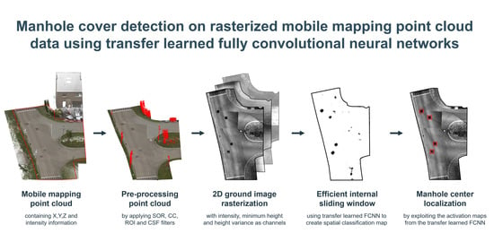
In this paper, we propose a fully automatic manhole cover detection framework to extract manhole covers from mobile mapping point cloud data. This approach makes use of deep learning networks that only require a small training dataset to achieve good detection results. The point cloud data are first rasterized into a ground image in order to simplify the detection task and use well-established image processing methods. Our ground image consists of three channels based on the lidar data: intensity, minimum height and height variance. While current research only works with intensity channels, our work investigates the use of additional geometric information as additional input channels for the ground image. Our method makes use of pre-trained classification convolutional neural networks (CNNs) which are transfer learned, only requiring a small labeled training dataset. The original network is first modified into a fully convolutional network in order to process larger images in an efficient way. This eliminates the use of a sliding window approach for the manhole cover detection. Additionally, the center of the manhole cover is predicted using the activation maps of the pooling layers of the network. Object detection and localization performance of this approach are evaluated on different CNN backbone architectures (AlexNet [8], VGG-16 [9], Inception-v3 [10] and ResNet-101 [11]). In summary, the main contributions of this paper are:

• Fully automatic manhole cover detection framework using transfer learned fully convolutional neural networks trained on a small dataset;
• Influence of additional geometric features as input channels for the CNN is assessed;
• Different backbone architectures (AlexNet, VGG-16, Inception-v3 and ResNet-101) are investigated for our proposed detection framework.

The remainder of this work is structured as follows. In Section 2, the related work on manhole cover detection using remote sensing data is discussed. This is followed by Section 3, in which we present our methodology. The experiments and results are presented and discussed in Section 4 and Section 5. Finally, the conclusions and future work are presented in Section 6.

2. Related Works

There are different methods to map or inventory manhole covers in a spatial database. When remote sensing data such as satellite imagery, UAV imagery or mobile mapping data (image and/or lidar data) are used, the acquisition time can be drastically reduced compared to traditional surveying techniques [3]. Although already more efficient, these methods would benefit more if the mapping of objects such as manhole covers could be automated, as this is still commonly performed manually. This is mainly because mapping for spatial databases requires high recall and precision performance. Research on mapping automation can be split up in three categories: image-based, lidar-based and combined image-/lidar-based methods. Because manhole covers have no distinctive 3D geometric features and object detection using 3D lidar data is more complex, most lidar-based methods convert the point cloud into a 2D intensity ground image [12,13,14,15]. By doing so, the point cloud detection problem becomes an image detection problem, making it possible to apply well-established image processing techniques. At first, more basic approaches were investigated using manually designed low-level features [12,16], but more machine and deep learning approaches have emerged in recent years, and their capabilities to learn complex high-level features have been used [13,14,17]. As R-CNN [18], YOLO [19] and SSD [20] are known to struggle with small objects, a more basic classification network and sliding window approach are generally applied. A summary of several manhole cover detection techniques are presented in this section.

In a recent study, manhole cover detection using mobile lidar data was investigated [6]. This method searches for manhole covers by filtering the point cloud with a pre-defined intensity interval, after which a best fitting bounding box is fitted to each cluster. As the dimensions of manhole covers are generally known, bounding boxes that are too small or too big are filtered out. Although this simple method performs well on raw point clouds and achieves usable results in their dataset, this method is not robust for other datasets, as it cannot distinguish the difference between a manhole cover or a dark intensity patch. Additionally, as soon as the manhole cover is partially occluded, the cluster is not square and is regarded as a false positive. Therefore, more complex image processing or deep learning approaches are needed.

In [16], a generic part-based detector model [21] was assessed on single view images from a moving van. These images were projected into an orthographic ground image such that the manhole covers had a circular shape. While the single-view approach resulted in poor recall and precision scores, their multiview approach proved more effective with a recall score of 93%. Such multiview approaches perform object detection on consecutive captured images and utilize their relative position to trace the manhole cover in 3D. This allows their approach to achieve higher recall and predict the 3D position with more accuracy and certainty. A similar single- and multiview approach was assessed on UAV-captured imagery in [22] using Haar-like features as input for a classifier to determine whether the image contained a sewer inlet or not. They compared three classifiers (support vector machine (SVM), logistic regression and neural network) in combination with a sliding window approach to perform the object detection. Their comparison showed that the neural network classifier resulted in the highest precision score compared to the other classifiers.

Yu et al. investigated several approaches to detect manhole covers from lidar data [12,13,14]. Each of his methods rasterizes the lidar data into an intensity ground image using the improved inverse distance weighted interpolation method proposed in [23]. In [12], Yu assessed a marked point model approach to detect manhole covers and sewer inlets in the ground image. This method, however, assumes that a manhole cover has a round shape and that a sewer inlet has a rectangular shape and attempts to fit these shapes around low-intensity patches of the ground image. While it was effective for clean road surfaces, this method failed on repaired roads where round or dark patches of new asphalt looked like manhole covers or sewer inlets. Their approach was improved in [13] using a machine learning approach. Instead of using low-level manually generated features, they opted to train a deep Boltzmann machine to generate high-level features from a local image patch. Afterward, these features were used in a sliding window approach with a random forest model to classify the patch as “manhole”, “sewer inlet” or “background”. This new machine learning approach outperformed the method from their previous work. In their most recent work [14], they investigated a deep learning approach. Instead of using a sliding window, the intensity ground image was segmented using a super-pixel-based strategy. Each segment was classified by their own designed convolutional network after which their marked point approach from [12] was used to accurately delineate the edges of the manhole covers. This new deep learning method slightly outperformed their previous machine learning method [13].

Other approaches use modified mobile mapping systems specifically designed to capture the road surface in high detail using lidar/image sensors [15] or a lidar profile scanner [24]. Both methods use a combination of manually designed low-level features such as HOG features, intensity histograms, PCA, etc. as input for their SVM classification method. While Ref. [15] used a sliding window approach on both intensity and colored ground images from lidar and imagery, Ref. [24] performed a super-pixel segmentation approach on the intensity ground image similar to [14]. Although the approach of [15] resulted in a good recall and precision score, this method uses dense and clear point cloud data from specifically designed mobile mapping systems. Lidar data from commercially available mobile mapping systems are more noisy and less dense, and they capture not only the road surface but the whole of the surroundings, making manhole detection more complex.

In 2019, a fully deep learning approach was assessed on high-resolution satellite imagery using a multilevel convolutional matching network [17]. Although this method achieves better results than traditional object detection methods such as R-CNN, YOLO or SDD, like so many deep learning methods, it needs a large quantity of training data to be successful. As no dedicated manhole cover training data exist, creating this dataset is time-consuming. For example, Ref. [15] labeled around 25,000 images to train their SVM classifier, Ref. [22] used 6500 labeled images and Ref. [13] used 15,000 images. While Ref. [17] only needed 1500 images for training, their training dataset did contain around 15,000 manhole cover bounding boxes. With the use of transfer learning on pre-trained networks, it is possible to achieve good results with only a fraction of the training data reducing time needed for manual labeling and the training of the network. This was demonstrated in [25] using ResNet-50 and Resnet-101 together as a backbone for the RetinaNet architecture using only 120 training images. Although it outperformed a Faster-RCNN implementation, these results are questionable, as the testing dataset only contained 36 images with 21 manhole covers, which does not represent a real-world example.

3. Methodology

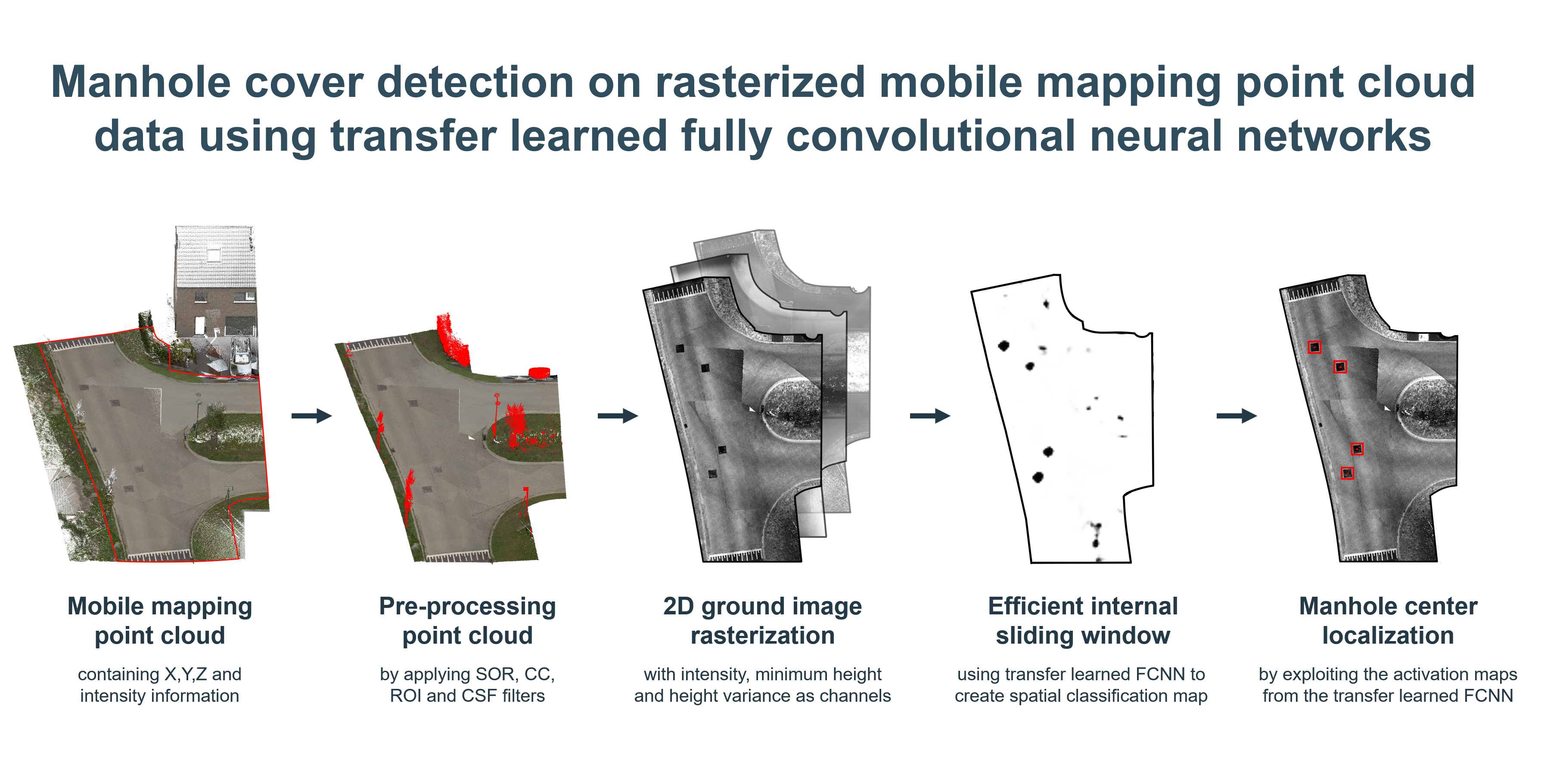
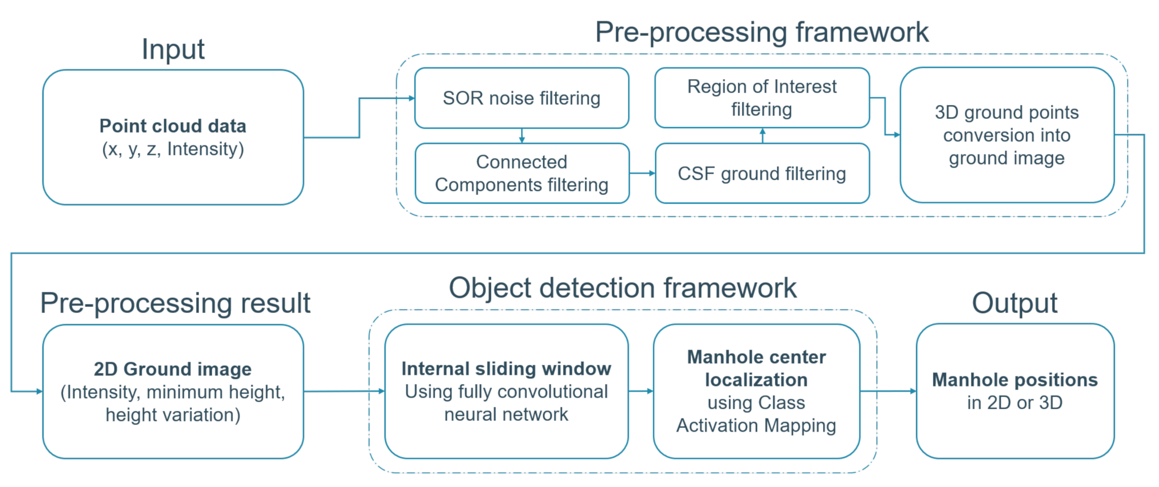
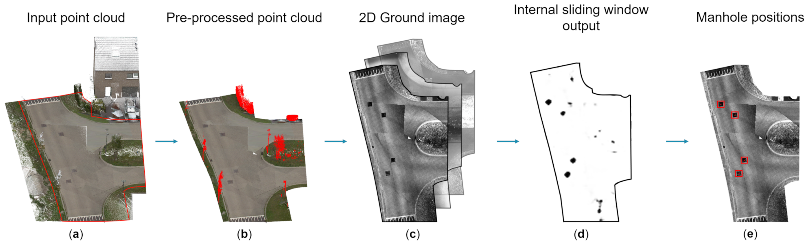
In this section, a detailed overview is presented of our proposed fully automatic manhole cover detection workflow. It contains two major components: the preprocessing framework and the object detection framework. The preprocessing framework consists of filtering steps that reduce the amount of noisy and unnecessary data for the subsequent processing steps, as well as the ground image conversion step that converts the 3D point cloud into a 2D ground image with intensity, minimum height and height as image channels. These images are then used as input of the object detection framework, which aims to find the manhole cover positions in them. In this framework, the images are processed by a fully convolutional neural network which simulates an internal sliding window producing a spatial classification output in an efficient way. This spatial output indicates where the network expects a manhole cover to be located. Using this result, the center of the manhole cover is predicted using the activation maps from the classification network. The complete workflow is shown in Figure 1, while some examples of intermediate results of the workflow are shown in Figure 2.

3.1. Preprocessing Framework

Because of the imperfections of lidar scanners and the influence of reflective surfaces or moving cars/people in the vicinity, mobile mapping point clouds of the public domain contain a considerable amount of noise or ghost points that influence the processing steps. In the preprocessing framework, these points are filtered by statistical outlier removal (SOR) and connected components (CC) filters. Additionally, mobile mapping systems capture all surroundings, including the road surface, road furniture, sidewalk, buildings, vegetation, etc. However, manhole covers only occur on the ground, making a large quantity of data obsolete. Therefore, a cloth simulation filter (CSF) is applied to segment the point cloud into “ground” and “nonground” points. Furthermore, an optional region of interest (RoI) filter is applied to further reduce the data that needs processing. Following the filtering steps, the 3D point cloud is rasterized into a georeferenced 2D ground image with three channels: intensity, height and height variance. These steps are discussed in detail in the following paragraph.

3.1.1. SOR, CC, CSF and RoI Filtering

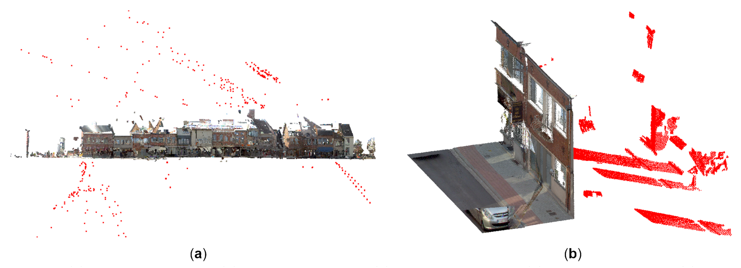
Mobile mapping point clouds include erroneous measurements caused by the imperfection of the laser scanner and the challenging environments such as reflective surfaces, moving cars and pedestrians. These errors can corrupt the object detection algorithms. This is especially the case for the CSF ground filtering which fails to produce usable results when noisy points are present under the road/ground surface. An example of these points is shown in Figure 3a. These points are commonly removed by applying a statistical, radius or multivariate outlier removal filter. The SOR filter, applied in our method, computes the average Euclidean distance of each point to its k neighbors plus the mean $\mu$ and standard deviation $\sigma$ of the average neighboring distance. A point is classified as outlier/noise when the average neighboring distance is greater than the maximum distance defined by $\mu +\alpha ·\sigma$. We found experimentally that the following parameters, $k=30$ and $\alpha =2$, removed the subterranean and sky noise points. However, high-density point clusters still remain, such as the ghosting points when measuring through a window (Figure 3b). Filtering these points is done by applying a connected components (CC) filter which segments the point cloud in different clusters separated by a minimum distance d and removes clusters smaller than the minimum cluster size $C_{min}$. In our implementation, we found that d = 0.3 m and $C_{min}$ = 10,000 works well to remove the majority of these ghost points without removing other relevant clusters.

The ground segmentation is performed by applying a cloth simulation filter [26]. This filter inverts the point cloud along the Z-direction and simulates a cloth being dropped on top of it. Depending on a few parameters such as the rigidity and resolution, the cloth follows the contours of the point cloud representing the digital terrain model (DTM). All points within a specified minimum distance of the DTM are classified as ground points. The main parameters of this filter are the grid resolution, rigidity and the classification threshold. The first determines the resolution of the cloth where a finer cloth will follow the terrain more closely than a coarse one. However, an overly fine resolution causes more nonground to be wrongly classified and results in longer processing times. The rigidity influences the stiffness of the cloth where a soft cloth will follow the terrain better. This parameter can be set to 1, 2 or 3 for steep slopes, terraced slopes or flat terrain, respectively. The classification threshold is the minimum distance to classify a point as ground or nonground. The optimal parameter settings are based on the findings in [26] and a few experimental tests. We chose 1, 3 and 0.3 m for the grid resolution, rigidity and classification threshold, respectively.

In our workflow, an optional region of interest filter can be applied to remove all points from the private domain as many large-scale databases only contain manhole covers in the public domain. The GRB, for example, contains a specific layer that delineates the public domain which is used to filter out points not within this layer. An example of this border is visualized in Figure 2a. This step reduces the quantity of data even more, resulting in faster processing of the following steps. As this is an optional step, the RoI filtering can be skipped when no boundary is available or necessary.

3.1.2. 2D Ground Image Conversion

Manhole covers have almost no height related features and are small objects in a mobile mapping point cloud. This makes it difficult to use point-cloud-based object detection methods. This is why we choose to rasterize the point cloud into a 2D georeferenced ground image. This reduces the amount of data that need processing while also simplifying the task to a image detection problem. As such, it is possible to use well-established image processing methods such as CNNs. Although most mobile lidar point cloud contain RGB data for each point, intensity information is preferred over the RGB information for the channels of the ground image. The difference in reflectivity between manhole covers and the road surface means that a black manhole cover is discernible on a black asphalt surface, which is impossible using RGB channels. However, different capturing positions and frequencies of the omnidirectional camera and laser scanner cause a variable shift between RGB data and intensity data. Although an accurate system calibration can reduce the influence of this error, imperfections of the lidar sensor and omnidirectional camera cause the error to persist. Additionally, passing vehicles or pedestrians result in false coloring of the road surface, which makes an RGB approach unreliable. For that reason, our implementation includes the following point cloud information as channels for the ground image: intensity, minimum height and height variance. The number of channels is limited as pre-trained models are designed for input images with three channels. Altering the number of input channels would require training from scratch and a massive training dataset. Although manhole covers have almost no height-related information, we aim to improve the precision performance of the network by including this information in the input image. As manhole covers occur all over the public domain, this complicates the detection problem. While manhole covers are flat, other areas such as curbs, grass, dirt, etc. have an uneven surface which is captured by the minimum height and height variance information. It is our estimation that the false positive detection rate of the whole workflow will decrease. A comparison between the performance of an intensity image and our IHV (intensity, height, variance) image is discussed in Section 4. The 2D ground image conversion in our implementation works as follows. First, the point cloud is tiled into sections of 50 by 50 m with 5 m overlap. Each tile is rasterized with a ground sampling distance of 2.5 cm which results in a 2000 by 2000 ground image. For each grid cell in the image, the corresponding point cloud position is calculated from which a 2D radius search groups all the points within 2.5 cm of the grid cell. From these points, the intensity values are computed with the method proposed in [23], which is based on an inverse distance weighted interpolation. This method computes a weighted intensity average of all points in the radius search by applying the following rules:

Rule 1:

a point with a higher intensity value has a greater weight.

Rule 2:

a point farther away from the center point of the grid cell has a smaller weight.

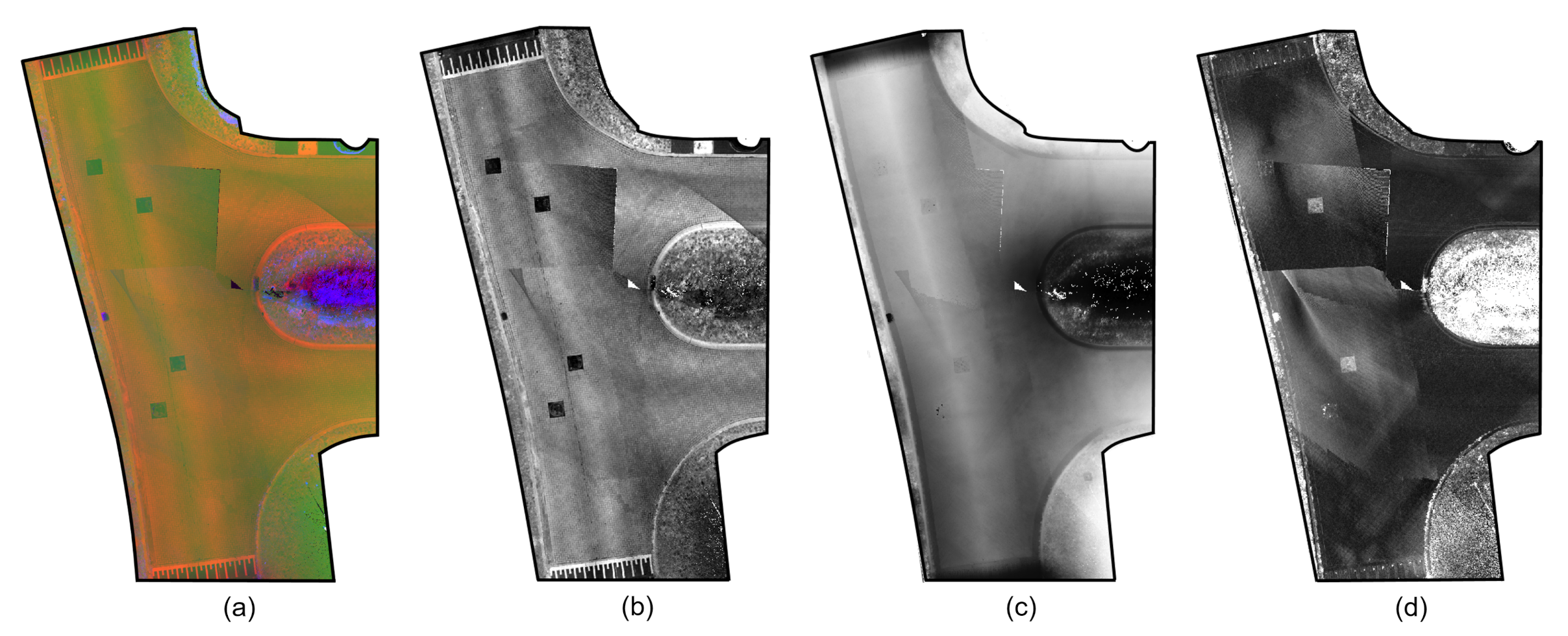
In our implementation, the weight coefficients of these rules $\alpha$ and $\beta$ are both set to 0.5. Additionally, the minimum height information of the grid cell is the minimum height value from the points in the radius search. The height variance information is the absolute height difference between the lowest and highest point from the corresponding cluster. As a result, the IHV ground image is created with three channels: intensity, minimum height and height variance. An example of such an image with the different channels is shown in Figure 4. Notice how some areas in the intensity channel do not display consistent values. Although the road surface is the same over the entire surface of the intersection, the variance in the intensity channels implies otherwise. This phenomenon commonly occurs at intersections where point cloud segments of different trajectories overlap with each other. As the intensity value of a measured point depends on the angle of incidence, this results in sudden changes in the intensity channels in areas with overlapping point clouds.

3.2. Object Detection Framework

The second component of our method is the object detection framework, consisting of the internal sliding window part and the manhole center localization. Both make use of the same modified transfer learned classification network to detect and accurately localize manhole covers in the ground image.

3.2.1. Internal Sliding Window

As traditional image object detection methods fail to perform robustly on small objects [17], our method performs a more commonly used sliding window approach that uses simpler classification models and has proved effective in previous research (see Section 2). A pre-trained ImageNet [27] classification network is transfer learned to label an image patch as “manhole” or “background”. A common transfer learning workflow is applied with the following steps. The first convolutional layers are frozen: their weights are not adjusted during training. These first layers contain the well-defined basic features trained from millions of images which would be erased or changed when not frozen during training, rendering the benefits of the pre-trained model obsolete. 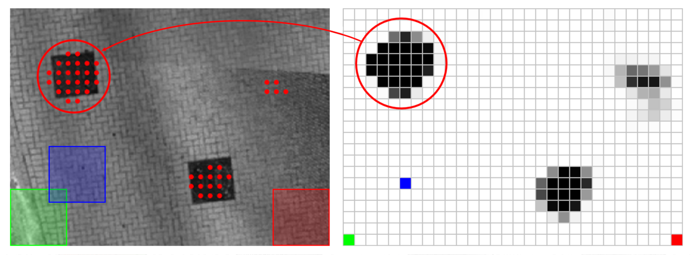The last “learning” layers are replaced to account for two output classes instead of the original 1000 from the ImageNet dataset [27]. While these layers are typically replaced by similar fully connected layers, we opt to replace them by fully convolutional layers, resulting in a fully convolutional network. This strategy is chosen because networks with fully connected layers are limited to processing images with a fixed size, while networks with fully convolutional layers can process larger images, generating a spatial classification map simulating an internal sliding window. An example of such a spatial classification map is shown in Figure 5. This internal sliding window approach based on Overfeat [28] has proved much more computationally efficient compared to a traditional sliding window.

3.2.2. Manhole Center Localization

The output of the fully convolutional network is a spatial classification map with size $R_o\times C_o$ which depends on the architecture of the network and the size of the input image defined by $R_i\times C_i$. As the fully convolutional network simulates an internal sliding window, each cell from the spatial classification map corresponds to a sliding window position of size $w\times w$ with w being the original input size of the classification network. The value in each cell corresponds to the classification score of the corresponding window located in that position. An example of three grid cells, highlighted in red, green and blue, and their corresponding windows are shown in Figure 5. Using the original image size and the resulting spatial classification map, the step size of the simulated sliding window can be computed using the following equation:

$$Ste{p}_{ver}=(R_i-w)/(R_o-1);Ste{p}_{hor}=(C_i-w)/(C_o-1)$$

(1)

With the horizontal and vertical step size, the sliding window position in the input image of each output cell at position $(r,c)$ in the spatial classification map is computed as follows:

$$r_i=\frac{w}{2}+(r-1)·Ste{p}_{ver};c_i=\frac{w}{2}+(c-1)·Ste{p}_{hor}$$

(2)

where $r_i$ and $c_i$ are the corresponding row and column coordinates in the input image. Figure 5 visualizes the window positions in the original input image that have a classification score greater than the defined classification threshold $T_{class}$. As can be seen in this image, there are large clusters of high classification scores (black), indicating a high possibility of a manhole cover, but there are also smaller clusters which are clearly false positives. In our approach, these clusters are detected by applying a clustering algorithm on the spatial classification map. This algorithm considers window positions with a classification score above the threshold $T_{class}$ and considers all adjacent windows to be in the same cluster. For the example in Figure 5, this results in three clusters. As false positive clusters are generally smaller than true positive clusters, clusters smaller than a user-defined cluster threshold $T_{cluster}$ are filtered out. In the subsequent processing steps, it is assumed that each cluster contains a manhole cover.

While common object detection approaches need bounding box training data to train a dedicated location network, our approach uses the same classification network to predict the position of the manhole in the image. This is done by applying a simplified version of class activation mapping, proposed in [29]. This approach uses the activation maps of pooling layers to highlight the region of the image which is most important for classifying the image as “manhole”. Additionally, this information can be used to predict the location of the manhole as follows. For each position of a cluster, the activation map of the corresponding window is extracted from the last pooling layer from the classification network. 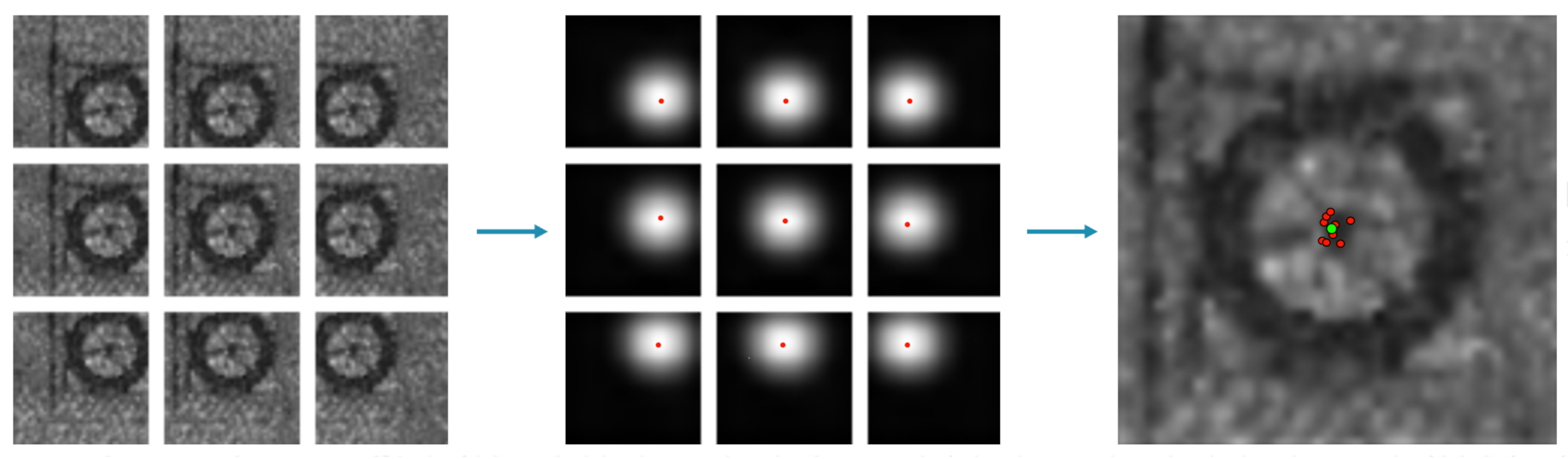In general, the activation map is a 3D matrix of size $row\times col\times depth$ which is flattened into a 2D matrix of size $row\times col$ by averaging the $depth$ dimension and also min-max normalizing to rescale the results to a value between 0 and 1. Figure 6 shows the normalized activation maps and the corresponding windows in a cluster. Notice how the highest activation values are located around the center of the manhole cover. To predict the center of the manhole, the weighted center of each normalized activation map is computed for each position in a cluster and converted into the image coordinates ($I_r,I_c$). In the end, the center of the manhole cover ($M_r,M_c$) is computed with a weighted average using the classification score S and the image coordinates of the activation map center ($Im{g}_r,Im{g}_c$) of each cluster position, using Equation (3).

$$M_r=\frac{{\displaystyle \sum _{i=1}^s}(S_i·I_r)}{{\displaystyle \sum _{i=1}^s}{S}_i};M_c=\frac{{\displaystyle \sum _{i=1}^s}(S_i·I_c)}{{\displaystyle \sum _{i=1}^s}{S}_i}$$

(3)

where s is the size of the cluster. Doing this for all clusters of the spatial classification map results in the positions of the different manhole covers. The localization algorithm is governed by two main parameters: cluster threshold $T_{cluster}$ and classification threshold $T_{class}$, which are optimized and analyzed in the results in Section 4.

4. Results

4.1. Training, Validation and Testing Datasets

All the data used for training and testing is captured by a Lynx mobile mapper SG equipped with the dual lidar system from the Lynx M1 Mobile Mapper. This setup captures points at a rate of 500 kHz with an accuracy of 8 mm up to 200 m to ensure a dense and accurate point cloud. The Lynx system was mounted on the roof of a Mitsubishi SUV driving at a speed of approximately 25–40 km/h during data acquisition. A more detailed summary and analysis of this system is presented in our previous work [30]. As no dedicated training or testing dataset for manhole cover detection is currently publicly available, we captured our own. The three mobile mapping datasets (rural, residential and urban datasets) from [30] were used to create the training and validation dataset to transfer learn the networks. Using the manhole covers positions in the GRB, the ground truth data were automatically extracted in the ground image. Although all images were manually checked and wrong images were removed, this semiautomatic approach was much more efficient compared to manually labeling the images. Additionally, “background” images were extracted, resulting in 443/190 and 455/195 images for the training/validation set for the “manhole” and “background” labels, respectively. Furthermore, a second training set with an additional 545 “background” images was created to investigate if these extra images would decrease false positive detections. In the remainder of the paper, dataset 1 refers to the dataset with equal manhole and background training images while dataset 2 refers to the dataset with the additional background training images. Both dataset 1 and 2 have the same validation dataset. Furthermore, we created two types of ground images for both datasets: one containing only the intensity channels and on with the IHV channels, resulting in four training datasets in total. To evaluate the object detection performance of the workflow, an additional testing dataset was captured with the same mobile mapping system. This dataset contains over 1 km of urban and residential roads and includes 73 manhole covers extracted from the GRB.

4.2. Network Selection and Training Parameters

In this work, we assessed the performance of four different network architectures including AlexNet [8], VGG-16 [9], Inception-v3 [10] and ResNet-101 [11]. From these four networks, AlexNet is considered the simplest with only eight layers compared to the “deeper” architecture of VGG-16 consisting of 16 layers. In contrast, Inception-v3 and ResNet-101 have a more complex architecture, as just adding convolutional layers results in a saturated accuracy at a certain depth that degrades rapidly when going even deeper [11]. Inception-v3 resolves this problem by building a wider network instead of deeper network using side-by-side convolutional computations in the same layer. ResNet, on the other hand, uses skip connections to achieve better results with deep networks with up to 152 layers.

Table 1. Summary of the main differences between AlexNet, VGG-16, Inception-v3 and ResNet-101.

Network	Depth	Parameters	ImageNet Top-5 Accuracy	Salient Feature
AlexNet	8	61 M	84.6%	First winning CNN
VGG-16	16	138 M	91.6%	Deeper than AlexNet
Inception-v3	48	24 M	94.4%	Side-by-side convolutions
ResNet-101	101	44.6 M	93.9%	Skip connections

summarizes the main differences including depth, number of parameters and ImageNet top-5 accuracy. The authors of [31] discovered that better ImageNet accuracy results in better transfer learning performance; thus, Inception is expected to outperform ResNet, VGG and AlexNet in that order.

Each network was transfer learned on their pre-trained ImageNet version using the four different training datasets utilizing the Deep Learning toolbox from MATLAB [32] on a computer with an Intel Xeon W-1233 processor, 32 GB of RAM and a Nvidia GTX 1080. All networks were trained using stochastic gradient descent optimization with a minibatch size of 52 for a total of 30 epochs. The initial learning rate was set between 0.001 and 0.0001, depending on the network/dataset combination, and it decayed after 10 epochs by a factor of 0.3. The momentum was set to 0.9 with a weight decay of 0.0001. Additionally, standard data augmentation such as rotation, scale and translation were performed on the dataset during training. On average, training took 2 min, 17 min, 22 min and 25 min for AlexNet, VGG-16, Inception-v3 and ResNet-101, respectively. Taking into account the depth of each network, it is clear that deeper/more complex networks take longer to train.

4.3. Classification Performance

The evaluation of the classification performance is done by comparing the accuracy, recall, precision and F-score from each network on the validation dataset. Instead of the commonly used $F_1$-score, which computes the harmonic mean between recall and precision, we opt to use a weighted F-score with the factor $\beta$ in which recall is considered $\beta$ times as important as precision. This is because a high recall score is of more importance than the precision score when mapping manhole covers in spatial databases. The $F_{\beta }$-score can be computed from Equation (4).

$$F_{\beta }=(1+{\beta }^2)·\frac{precision·recall}{({\beta }^2·precision)+recall}$$

(4)

In terms of the $F_2$-score, this means that recall is twice as important as precision.

Table 2. Accuracy, recall, precision and $F_2$-score for AlexNet, VGG-16, Inception-v3 and ResNet-101 trained on dataset 1 and 2 for intensity and IHV images. The highest scores for each dataset are shown in bold.

Network	Dataset	Image	Accuracy	Recall	Precision	F2-Score
AlexNet	1	Intensity	0.969	0.963	0.973	0.965
VGG-16	1	Intensity	0.990	0.995	0.984	0.993
Inception-v3	1	Intensity	0.979	0.989	0.969	0.985
ResNet-101	1	Intensity	0.995	0.995	0.995	0.995
AlexNet	2	Intensity	0.974	0.974	0.974	0.974
VGG-16	2	Intensity	0.992	0.984	1.000	0.987
Inception-v3	2	Intensity	0.982	0.979	0.984	0.980
ResNet-101	2	Intensity	0.997	0.995	1.000	0.996
AlexNet	1	IHV	0.911	0.963	0.871	0.943
VGG-16	1	IHV	0.961	0.974	0.949	0.969
Inception-v3	1	IHV	0.961	0.979	0.944	0.972
ResNet-101	1	IHV	0.914	1.000	0.852	0.966
AlexNet	2	IHV	0.948	0.979	0.921	0.967
VGG-16	2	IHV	0.971	0.979	0.964	0.976
Inception-v3	2	IHV	0.961	0.989	0.935	0.978
ResNet-101	2	IHV	0.961	0.995	0.931	0.982

shows the validation results for the different networks. When comparing the intensity-trained networks against IHV-trained networks, the former outperform the latter, especially in terms of precision. Our assumption that the extra geometric features would improve the precision score does not hold. When comparing the results of dataset 1 to those corresponding to dataset 2, the intensity-trained networks perform similarly, meaning the extra “background” images have no significant influence. In contrast, the IHV-trained networks show a significant precision improvement of 5.6% and 9.7% when trained on the extra “background” images for the AlexNet and ResNet architectures, respectively. The best performance score for each dataset combination is shown in bold in this table. In general, ResNet-101 performs the best on the validation dataset, with VGG-16 and Inception-v3 close behind, while AlexNet performs the worst for each dataset combination. This indicates that more complex networks outperform the simpler shallow AlexNet architecture.

In addition to the classification performance, the sliding window performance on ground images is also relevant. This performance is computed for each network on a small test image as is shown in

Table 3. Visualization of the sliding window positions with a classification score greater than the classification threshold ($T_{class}$ = 0.5) for the different networks and training datasets. The two manhole covers in the image are indicated by the green bounding box.

Network	Dataset 1 Int.	Dataset 2 Int.	Dataset 1 IHV	Dataset 2 IHV
AlexNet
VGG-16
Inception-v3
ResNet-101

. Each red point corresponds to a sliding window position with a classification score above 0.5. When analysing the AlexNet results, it is clear that, although the performance on the validation set was relatively high, the network does not perform robustly on larger images. For each dataset combination, there are large clusters of false positive classifications resulting in a low precision score and longer processing times. In contrast, the VGG-16 results look promising with clear clusters around each manhole cover and a few small false positive clusters, which are easily filtered out based on cluster size. However, it should be noted that the majority of these false positive clusters overlap with inspection covers on the side walk. These smaller covers are used for inspecting gas, water or private sewage lines and look similar to manhole covers. Additionally, these are not commonly mapped in large spatial databases and therefore need to be filtered out. Similar inspection cover errors are present in the Inception-v3 results, although these clusters are much bigger. As these have sizes similar to the true positive clusters, filtering based on cluster size is not an option. Additionally, more noisy false positive clusters are present compared to the VGG-16 results. The ResNet-101 results show similar inspection cover errors and large false positive clusters, especially for the IHV-trained networks. Additionally, the networks struggle to classify all manhole covers in the test image while achieving the highest recall scores on the validation dataset in Table 2.

These results show that a high classification score does not automatically correspond to good sliding window performance on a larger image. In general, the VGG-16 architecture is the only network performing consistently in terms of classification and sliding window across the different dataset combinations. Therefore, only the VGG-16 networks are analyzed on the testing dataset, as these are the most likely to achieve good object detection results.

4.4. Manhole Detection Performance

Our proposed object detection and localization method is evaluated on the additional testing dataset containing 73 manhole covers. A predicted manhole cover position is considered a true positive when it is within a distance of 36 pixels (=90 cm) of the ground truth center point. This distance corresponds to the average size of a manhole cover found in the public domain. For each VGG-16 network, the classification threshold $T_{class}$ and cluster threshold $T_{cluster}$ are optimized for two scenarios (maximum $F_2$-score and maximum recall score). The optimal localization parameters and corresponding recall, precision and $F_2$-score are shown in

Table 4. Summary of the object detection results (recall, precision and $F_2$-score) with the corresponding classification threshold $T_{class}$ and cluster threshold $T_{cluster}$ for the whole public domain. The results and optimal parameters are displayed for both the maximal $F_2$-score and maximal recall score.

Dataset	Maximum ${\mathit{F}}_2$-Score Optimization					Maximum Recall Optimization
	Recall	Precision	${\mathit{F}}_2$-Score	${\mathit{T}}_{\mathit{class}}$	${\mathit{T}}_{\mathit{cluster}}$	Recall	Precision	${\mathit{F}}_2$-Score	${\mathit{T}}_{\mathit{class}}$	${\mathit{T}}_{\mathit{cluster}}$
1 Int.	0.904	0.680	0.848	0.8	10	1.000	0.237	0.608	0.5	2
2 Int.	0.932	0.482	0.785	0.9	16	1.000	0.258	0.635	0.8	9
1 IHV	0.699	0.183	0.447	0.2	19	0.973	0.077	0.293	0.7	1
2 IHV	0.781	0.209	0.504	0.3	18	0.973	0.086	0.317	0.7	1

. From the maximum $F_2$-score results, it is clear that the intensity-trained networks outperform the IHV-trained networks, as was the case in terms of classification performance. The additional geometric features result in a significantly lower recall score and an unusable precision score of around 0.2. This means that only one in five predicted manhole covers is actually a manhole cover and only 70%–80% of manhole covers are detected. In contrast, both intensity-trained networks achieve a +90% recall score while achieving a 68% and 48% precision score for dataset 1 and 2, respectively. In this case, the additional “background” images resulted in more false positive detections while the opposite was intended. Similar observations are made in the case of maximum recall optimization where the intensity-trained networks outperform the IHV-trained networks. When recall is of utmost importance, the intensity-trained networks are able to detect all manhole covers with a corresponding low precision score of 25%. While the IHV-trained networks also achieve a high recall, the precision score equals to 8%.

The detection results for the maximum $F_2$-score configuration are shown in Figure 7 on a small section of the testing dataset. True positive manhole cover predictions are depicted with a green cross, false positives with a red cross. The ground truth manhole covers are indicated with a green or red bounding box depending if they are detected or not. These images illustrate the varying recall scores of the networks where the IHV-trained networks perform slightly worse as is visible in Figure 7d. Additionally, the intensity-trained networks show far fewer false positives compared to the IHV-trained networks. Some of these false positives are caused by the presence of small inspection covers or storm drains. However, the majority of false positives are positioned in areas where it is not clear why they were classified as “manhole”. Notice how, in general, these false positives occur on the sidewalks or the side of the road while the networks perform quite well on the road surface. Although the training dataset contains an equal number of “background” images of the road surface or the side of the road, there is a clear performance difference. Therefore, the precision, recall and $F_2$-score are also computed when only taking into account the detections on the road surface. This is similar to application of the optional region of interest filters during the preprocessing framework as described in Section 3.1.

Table 5. Summary of the object detection results (recall, precision and $F_2$-score) with the corresponding classification threshold $T_{class}$ and cluster threshold $T_{cluster}$ when only considering the detection on the road surface. The results and optimal parameters are displayed for both the maximal $F_2$-score and maximal recall score.

Dataset	Maximum F2-Score Optimization					Maximum Recall Optimization
	Recall	Precision	F2-Score	${\mathit{T}}_{\mathit{class}}$	${\mathit{T}}_{\mathit{cluster}}$	Recall	Precision	F2-Score	${\mathit{T}}_{\mathit{class}}$	${\mathit{T}}_{\mathit{cluster}}$
1 Int.	0.945	0.863	0.927	0.9	5	1.000	0.646	0.901	0.5	2
2 Int.	0.973	0.973	0.973	0.9	12	1.000	0.849	0.966	0.8	9
1 IHV	0.932	0.618	0.846	0.7	5	0.973	0.415	0.767	0.7	1
2 IHV	0.932	0.654	0.859	0.9	2	0.973	0.504	0.820	0.7	1

summarizes the same performance scores for the different networks only considering the detection on the road surface for the different networks. When compared to Table 4, it is immediately clear how well the networks perform when only the road surface is considered. With the new optimal location parameters, recall achieves 93.2% for the IHV-trained networks with the precision score improving to around 60%–65%. While this is a significant improvement over the previous results, this only matches the performance of the intensity-trained network on dataset 1 on the whole public domain. In contrast, the intensity-trained network outperforms the IHV-trained networks by a large margin. While both intensity-trained networks improved, it is especially the intensity-trained network on the extra “background” images that achieves a high recall and precision score of 97.3%. In the case of the maximum recall optimization when only considering the road surface, recall scores are similar but with a much higher precision score. Similarly, as with the maximum $F_2$-score optimization, the intensity-trained network on dataset 2 performs the best and achieve an impressive 85% precision score with a 100% recall score. In both the maximum $F_2$-score and recall optimization, we notice a considerable improvement by training with additional “background” images.

4.5. Manhole Localization Performance

While most research documents detection performance in terms of recall and precision score, the localization accuracy of the center of the manhole cover is generally ignored. This is important as spatial databases usually require a specific level of accuracy for each object. In this section, the location accuracy of our approach is investigated by comparing the predicted center position to the ground truth center position determined from the GRB. These accuracy statistics are computed using the detection results and using the maximum $F_2$-score optimization from Table 4.

For each network, the mean error, standard deviation, root-mean-square error (RMSE) and 95% confidence interval (=2 × RMSE) are computed. The results are shown in

Table 6. Summary of the error results (mean, standard deviation, root-mean-square error and 95% confidence interval) for the different trained VGG-16 networks. Both the errors, in pixels and centimeters, are displayed, taking into account the GSD of 2.5 cm.

Dataset	Sample Size	Mean Error	Std. Dev	RMSE	95% Conf. Int.
1 Int.	66	2.8 pix/7.1 cm	1.7 pix/4.3 cm	3.3 pix/8.3 cm	6.6 pix/16.5 cm
2 Int.	68	3.1 pix/7.7 cm	1.9 pix/4.8 cm	3.6 pix/9.1 cm	7.3 pix/18.1 cm
1 IHV	51	5.1 pix/12.7 cm	3.9 pix/9.6 cm	6.4 pix/15.9 cm	12.7 pix/31.8 cm
2 IHV	57	5.4 pix/13.6 cm	3.1 pix/7.7 cm	6.2 pix/15.6 cm	12.5 pix/31.2 cm

, both in pixels and centimeters, taking the GSD of 2.5 cm into account. From these results, it is clear that, like the object detection performance, the intensity-trained networks outperform the IHV-trained networks with an average RMSE of 8.7 cm and 15.8 cm, respectively. Additionally, there is a noticeable performance difference between the intensity-trained networks on dataset 1 or 2. Although both datasets contain the same “manhole” training images, the additional “background” training images in dataset 2 degrade the 95% confidence interval from 16.5 cm to 18.1 cm. Because of the difference in sample size, this is not the case for the IHV-trained networks. When only taking the manhole covers detected by both IHV-trained networks into account, a similar performance difference is observed. These differences in accuracy become clearer when plotted on a scaled picture of a manhole cover as in Figure 8. As reference, a manhole cover is, in general, 90 cm or 36 pixels wide. Figure 8 allows to observe the performance difference between the intensity-/IHV-trained networks and the dataset-1-/2-trained networks by comparing the 95% confidence interval displayed by the red circle. There is a slight systematic deviation on the location prediction toward the upper-right corner. This unpredictable error is the downside of using a CAM-based localization approach. While the activation maps indicate the region of interest most important to classify the image and can be used for coarse localization of an object, this region does not necessarily correspond with the center position of the manhole cover, causing a systematic error on the location performance. Nevertheless, our approach is able to predict the manhole center with a 95% confidence interval of 16.5 cm using the intensity-trained VGG-16 network on dataset 1. In combination with the best manhole detection performance on the public domain, this network ensures the best results to map manhole covers for a spatial database.

In order to determine if the results are accurate enough for the GRB, a more detailed analysis must be performed. The GRB specification state that the errors in the X and Y directions between the control/ground truth positions and predicted position must follow a certain distribution [1]. This distribution is defined by an object-specific standard deviation ${\sigma }_{GRB}$ computed as follows:

$${\sigma }_{GRB}=\sqrt{{\sigma }_m^2+{\sigma }_{cm}^2+2{\sigma }_i^2}$$

(5)

where ${\sigma }_m$ is the requested measurement accuracy in X and Y of 0.03 m, ${\sigma }_{cm}$ the control/ground truth measurement accuracy in X and Y of 0.03 m and ${\sigma }_i$ the object-specific accuracy which is 0.007 m for manhole covers. All together, this results in a manhole-specific standard deviation ${\sigma }_{GRB}$ of 0.044 m. Using this standard deviation, the different GRB specified accuracy intervals of the distribution are defined as shown in

Table 7. The distribution results per accuracy interval for the different VGG-16 networks. Results conforming to the GRB requirements are shown in bold.

Dataset	Sample Size	${\mathit{\sigma }}_{\mathbf{GRB}}\times 1$ = 4.4 cm	${\mathit{\sigma }}_{\mathbf{GRB}}\times 1.2$ = 5.2 cm	${\mathit{\sigma }}_{\mathbf{GRB}}\times 1.5$ = 6.5 cm	${\mathit{\sigma }}_{\mathbf{GRB}}\times 2$ = 8.7 cm	${\mathit{\sigma }}_{\mathbf{GRB}}\times 3$ = 13.1 cm	${\mathit{\sigma }}_{\mathbf{GRB}}\times 4$ = 17.4 cm
1 Int.	66	63.6%	70.5%	77.3%	87.1%	96.2%	98.5%
2 Int.	68	53.8%	62.9%	73.5%	87.1%	96.2%	99.2%
1 IHV	51	35.0%	40.0%	51.0%	63.0%	83.0%	90.0%
2 IHV	57	35.1%	37.7%	44.7%	53.5%	73.7%	91.2%
GRB requirements:		60%	70%	80%	90%	95%	100%

. As an example, the GRB requires at least 60% of X and Y errors between ground truth and measured manhole center are smaller than ${\sigma }_{GRB}\times 1$ which deviates slightly from a normal distribution. Additionally, no less than 95% of X and Y errors must be smaller than ${\sigma }_{GRB}\times 3$. For a dataset of manhole covers to be accepted to update the GRB, all six accuracy interval requirements must be met. The distribution percentages for each VGG-16 network are presented in Table 7, with each result shown in bold when conforming to the GRB requirement. From these results, it is clear that only the intensity-trained networks comply with a few accuracy intervals. Although these results are not accurate enough for the GRB, an improved localization framework or additional fine-tuning of the prediction in postprocessing would improve these results and ensures the accuracy needed for the GRB. A few suggestions are presented in Section 5.

5. Discussion

Although multiple studies have looked into mapping manhole covers from mobile mapping point cloud data, no dedicated testing dataset exists to easily compare different methods. Fortunately, the research conducted by Yu et al. [12,13,14] has several similarities with our approach, such as the detection, which is performed on intensity ground images rasterized from mobile point cloud data. These different methods are discussed in detail in Section 2 and can be described as the marked-points-based method [12], the deep Boltzmann machine/random forest and sliding window method [13] and the super-pixel and CNN method [14]. 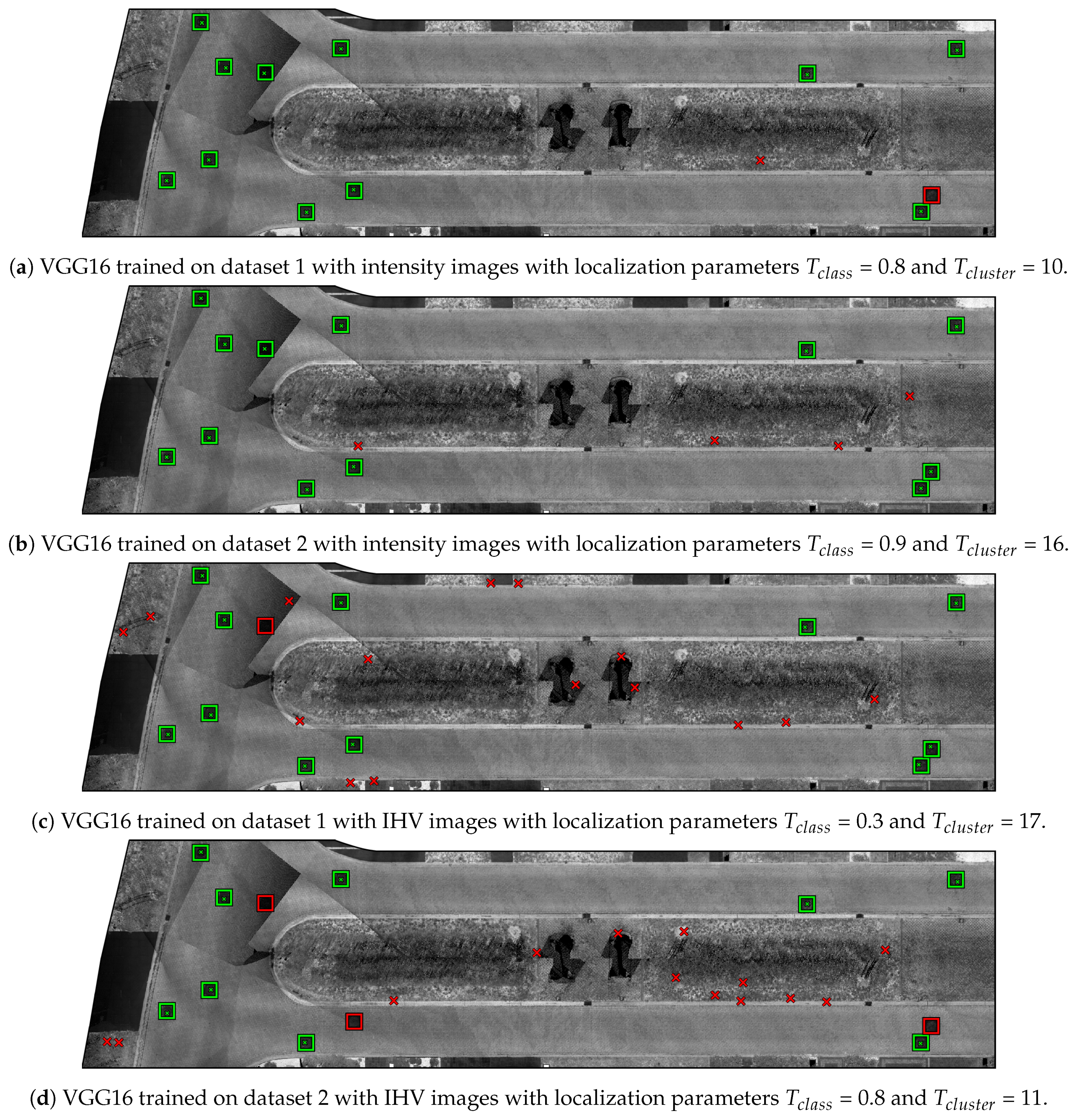In the following, only the detection results from Table 5 are considered as all methods of Yu et al. only detect manhole covers on the road surface. Note that the methods of Yu et al. are trained and evaluated on a much larger dataset compared to ours. Because of this, our results are not as reliable compared to previous research. However, our test dataset does contain a diverse environment, varying from urban to residential areas, representing a real-world example, and it is sufficiently large to evaluate our proposed method.

Table 8. Summary of the detection results of different manhole cover detection approaches on intensity ground images.

Method	# Training Images *	# Manhole Covers	Recall	Precision	${\mathit{F}}_1$-Score	${\mathit{F}}_2$-Score
Yu et al. [12]	NA	491	0.896	0.903	0.900	0.898
Yu et al. [13]	7820/7820	491	0.953	0.955	0.954	0.954
Yu et al. [14]	2200/2200	491	0.965	0.961	0.963	0.965
Proposed	443/1000	73	0.973	0.973	0.973	0.973
Proposed	443/1000	73	1.000	0.849	0.918	0.966

* (manhole training images)/(background training images).

lists the manhole detection results for each approach, including our maximum $F_2$-score and recall optimization of the intensity-trained VGG-16 network on dataset 2. Of these methods, the more traditional model-based detection approach achieves the lowest recall, $F_1$- and $F_2$-score. The DBM/RF machine learning approach significantly improves these results by using high-level feature generation. The deep learning approaches improve these results even more. Our proposed method with the VGG-16 intensity-trained network on dataset 2 and $F_2$-score optimization achieves the best performance results compared to the other methods. This is quite impressive, considering that our method only needs a fraction of the positive “manhole” training images because of transfer learning. Although our approach using intensity-trained networks achieves high detection scores on the road surface, the same cannot be said for the detection results on the whole public domain or the IHV-trained networks. A few remarks and possible solutions to improve these results are discussed below.

Our assumption that the additional geometric channels in the ground image would help detection does not hold up. We still believe geometric features can be used to enhance the precision performance, although not with transfer learning using a small training dataset. Instead, training a network from scratch, which would require much more data, could result in better detection results as the network would learn specific features from the IHV ground images. An alternative solution is to use the intensity-trained networks to detect the manhole covers with a high recall score and postprocess these results using common geometric features to filter out false positives. Additionally, there was a significant detection performance difference between the road surface and the rest of the public domain. This is mainly because the appearance of the public domain in the ground image has much more variation. Our results also indicated that training on additional “background” images slightly improves the results. Although this dataset contains a slight class imbalance, 1:2 manhole/background ratio, adding more “background” images to the training dataset is simply not going to further improve the results. This causes a severe class imbalance, 1:5 or 1:10 manhole/background ratio, and drastically degrades the manhole cover detection performance. Fortunately, different methods exist to address class imbalance on a dataset level or classifier level [33].

In addition to the object detection performance, the manhole center location also needs improvement to comply with the accuracy requirements of large-scale spatial databases such as the GRB. A dedicated localization network can be trained to determine the center of a manhole based on the ground image. This approach requires additional manual tagging of the manhole centers in our dataset as it only contains labeled images. As a network will always be less accurate than the dataset it was trained on, the manhole positions in the GRB are not accurate enough to automatically create this dataset. On the other hand, a postprocessing step to fine-tune the center position can be performed on the detection results of our approach. Some examples of such methods are the marked point [12,14] and GraphCut segmentation [16] approach to accurately delineate each manhole cover. If not successful, a semiautomatic approach can be employed where the user fine-tunes the predicted position manually. This way, the user can also filter out any false positive results and check all detection results, which will most likely be necessary anyway in a production environment, no matter how accurate the detection methods become.

6. Conclusions

In this paper, a fully automatic manhole cover detection method is presented to extract manhole covers from mobile mapping lidar data consisting of two components. First, the preprocessing framework removes the noisy and ghosting points, segments the point cloud into “ground” or “nonground” and rasterizes the “ground” points into a ground image with channels intensity, minimum height and height variance (IHV). Second, the object detection framework uses these ground images as input for a transfer learned fully convolutional network which simulates an internal sliding window and outputs a spatial classification map. This map indicates where the network expects a manhole cover to be located and is used to accurately determine the center position of each manhole cover using the activation maps of the last pooling layer. In this work, different backbone architectures (AlexNet, VGG-16, Inception-v3 and ResNet-101) are assessed after transfer learning on relatively small datasets with dataset 1 only containing the intensity channel while dataset 2 contains IHV images. Furthermore, the influence of additional “background” training images is investigated.

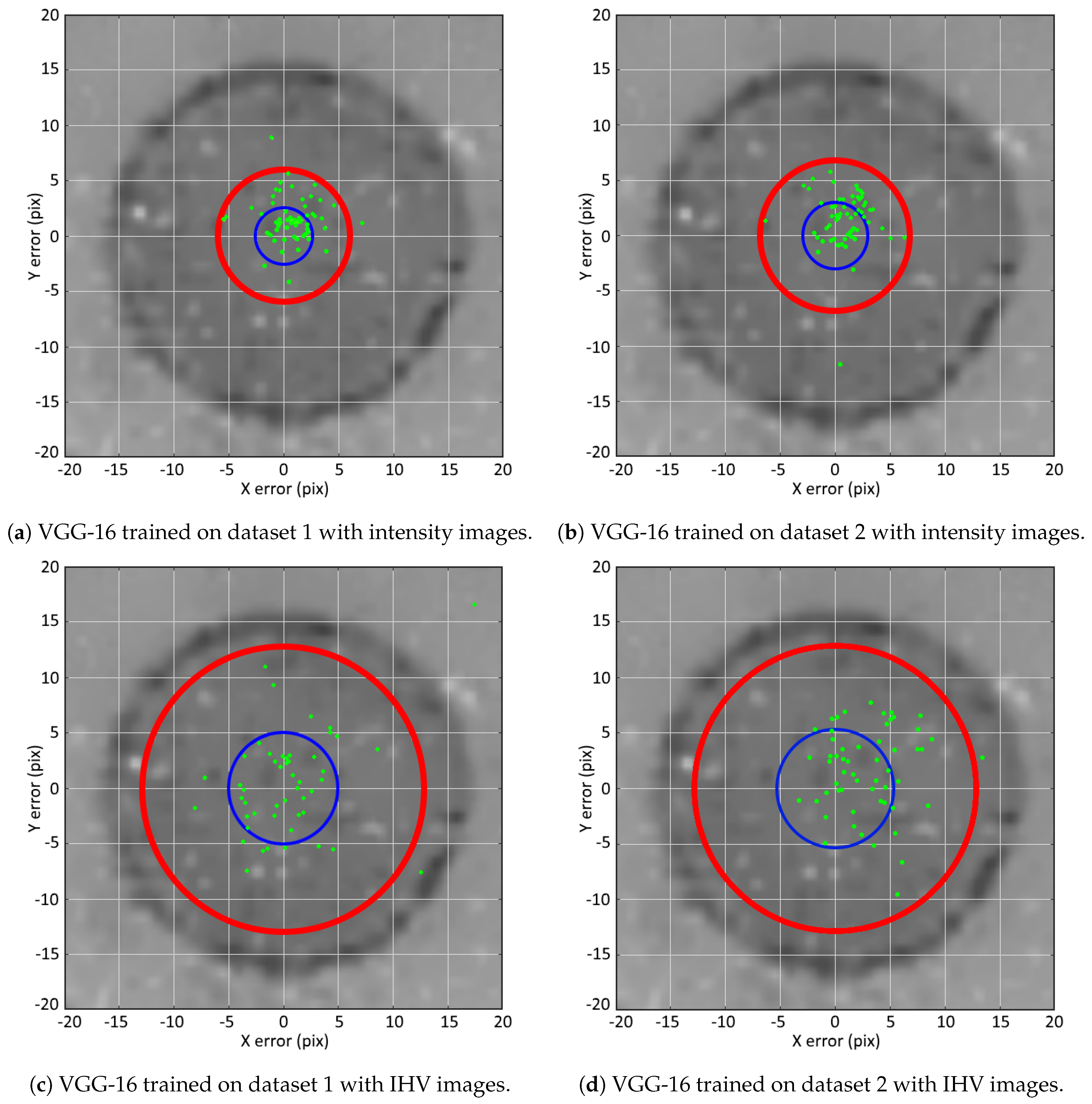
Our method is tested in a variety of experiments. First, the classification and sliding window performance of each network is compared which reveals that a high classification score does not automatically results in a good sliding window performance. The VGG-16 architecture performs the most consistent in both tasks. Next, the object detection performance of the VGG-16 networks is assessed on a dedicated testing dataset containing 73 manhole covers. Although our intention was to detect manhole covers all over the public domain, we noticed a significant detection performance difference between the false positive detection rate on the road surface and the rest of the public domain. When only taking into account the detection on the road surface, the best detection results are achieved with the intensity trained network on dataset 1, achieving a recall, precision and $F_2$-score of 0.973, 0.973 and 0.973, respectively. Overall, the experiments show that the networks trained on the IHV channels with geometric information degrade the detection performance instead of improving it. Furthermore, training with additional “background” images improves the precision score slightly. Last, the localization performance is compared, using the ground truth manhole center positions. Again, the intensity-trained networks outperform the IHV-trained networks with a RMSE of around 8.7 cm and 15.8 cm, respectively. Additionally, training on more “background” images resulted in a poorer localization accuracy. Our approach achieves a horizontal 95% confidence interval of 16.5 cm for the intensity-trained VGG-16 network on dataset 1, which almost complies with the GRB accuracy requirements.

Our future work will focus on improving the localization performance accuracy by implementing a dedicated-localization-network- or model-based approach. While currently our approach only uses the mobile point cloud data, future work will also focus on manhole cover detection on omnidirectional mobile mapping images. This image-based approach has the advantage that a manhole cover can be detected in multiple images, resulting in better detection results. Additionally, a combined image- and lidar-based approach will be investigated to further enhance the results. This approach will improve the recall performance, as a manhole cover can be detected in both the omnidirectional image and the lidar data. Additionally, detecting a manhole cover in both the image and lidar data increases the reliability of the result, creating a more robust detection framework.

References

1. Informatie Vlaanderen. Basiskaart Vlaanderen (GRB). Available online: https://overheid.vlaanderen.be/informatie-vlaanderen/producten-diensten/basiskaart-vlaanderen-grb (accessed on 31 January 2020).
2. Dutch Digital Government. Basisregistratie Grootschalige Topografie (BGT). Available online: https://www.digitaleoverheid.nl/overzicht-van-alle-onderwerpen/basisregistraties-en-afsprakenstelsels/inhoud-basisregistraties/bgt (accessed on 31 January 2020).
3. Jalayer, M.; Zhou, H.; Gong, J.; Hu, S.; Grinter, M. A Comprehensive Assessment of Highway Inventory Data Collection Methods for Implementing Highway Safety Manual. J. Transp. Res. Forum 2014, 53, 73–92. [Google Scholar] [CrossRef] [Green Version]
4. Guan, H.; Li, J.; Cao, S.; Yu, Y. Use of mobile LiDAR in road information inventory: A review. Int. J. Image Data Fusion 2016, 7, 219–242. [Google Scholar] [CrossRef]
5. Sairam, N.; Nagarajan, S.; Ornitz, S. Development of Mobile Mapping System for 3D Road Asset Inventory. Sensors 2016, 16, 367. [Google Scholar] [CrossRef] [PubMed] [Green Version]
6. Alshaiba, O.; Núñez-Andrés, M.A.; Lantada, N. Automatic manhole extraction from MMS data to update basemaps. Autom. Constr. 2020, 113, 103110. [Google Scholar] [CrossRef]
7. Ma, L.; Li, Y.; Li, J.; Wang, C.; Wang, R.; Chapman, M.A. Mobile laser scanned point-clouds for road object detection and extraction: A review. Remote Sens. 2018, 10, 1531. [Google Scholar] [CrossRef] [Green Version]
8. Krizhevsky, A.; Sutskever, I.; Hinton, G.E. ImageNet Classification with Deep Convolutional Neural Networks. Commun. ACM 2017, 60, 84–90. [Google Scholar] [CrossRef]
9. Simonyan, K.; Zisserman, A. Very deep convolutional networks for large-scale image recognition. In Proceedings of the International Conference on Learning Representations, San Diego, CA, USA, 7–9 May 2015; pp. 1–14. [Google Scholar]
10. Szegedy, C.; Vanhoucke, V.; Ioffe, S.; Shlens, J.; Wojna, Z. Rethinking the Inception Architecture for Computer Vision. In Proceedings of the IEEE Conference on Computer Vision and Pattern Recognition, Las Vegas, NV, USA, 27–30 June 2016; pp. 2818–2826. [Google Scholar]
11. He, K.; Zhang, X.; Ren, S.; Sun, J. Deep residual learning for image recognition. In Proceedings of the IEEE Conference on Computer Vision and Pattern Recognition, Las Vegas, NV, USA, 27–30 June 2016; pp. 770–778. [Google Scholar] [CrossRef] [Green Version]
12. Yu, Y.; Li, J.; Guan, H.; Wang, C.; Yu, J. Automated detection of road manhole and sewer well covers from mobile LiDAR point clouds. IEEE Geosci. Remote Sens. Lett. 2014, 11, 1549–1553. [Google Scholar] [CrossRef]
13. Yu, Y.; Guan, H.; Ji, Z. Automated Detection of Urban Road Manhole Covers Using Mobile Laser Scanning Data. IEEE Trans. Intell. Transp. Syst. 2015, 16, 3258–3269. [Google Scholar] [CrossRef]
14. Yu, Y.; Guan, H.; Li, D.; Jin, C.; Wang, C.; Li, J. Road Manhole Cover Delineation Using Mobile Laser Scanning Point Cloud Data. IEEE Geosci. Remote Sens. Lett. 2020, 17, 152–156. [Google Scholar] [CrossRef]
15. Wei, Z.; Yang, M.; Wang, L.; Ma, H.; Chen, X.; Zhong, R. Customized Mobile LiDAR System for Manhole Cover Detection and Identification. Sensors 2019, 19, 2422. [Google Scholar] [CrossRef] [PubMed] [Green Version]
16. Timofte, R.; Van Gool, L. Multi-view Manhole Detection, Recognition, and 3D Localisation. In Proceedings of the IEEE International Conference on Computer Vision Workshop, Barcelona, Spain, 6–13 November 2011; pp. 188–195. [Google Scholar]
17. Liu, W.; Cheng, D.; Yin, P.; Yang, M.; Li, E.; Xie, M.; Zhang, L. Small Manhole Cover Detection in Remote Sensing Imagery with Deep Convolutional Neural Networks. ISPRS Int. J. Geo-Inf. 2019, 8, 49. [Google Scholar] [CrossRef] [Green Version]
18. Girshick, R.; Donahue, J.; Darrell, T.; Malik, J. Rich feature hierarchies for accurate object detection and semantic segmentation. In Proceedings of the IEEE Conference on Computer Vision and Pattern Recognition, Columbus, OH, USA, 23–28 June 2014; pp. 580–587. [Google Scholar]
19. Redmon, J.; Divvala, S.; Girshick, R.; Farhadi, A. You only look once: Unified, real-time object detection. In Proceedings of the IEEE Conference on Computer Vision and Pattern Recognition, Las Vegas, NV, USA, 27–30 June 2016; pp. 779–788. [Google Scholar]
20. Liu, W.; Anguelov, D.; Erhan, D.; Szegedy, C.; Reed, S.; Fu, C.Y.; Berg, A.C. SSD: Single shot multibox detector. In Proceedings of the European Conference on Computer Vision, Amsterdam, The Netherlands, 8–16 October 2016; Volume 9905. [Google Scholar]
21. Felzenszwalb, P.F.; Girshick, R.B.; McAllester, D.; Ramanan, D. Object Detection with Discriminatively Trained Part Based Models. IEEE Trans. Pattern Anal. Mach. Intell. 2010, 32, 1627–1645. [Google Scholar] [CrossRef] [PubMed] [Green Version]
22. Moy de Virty, M.; Schnidler, K.; Rieckermann, J.; Leitão, J.P. Sewer Inlet Localization in UAV Image Clouds: Improving Performance with Multiview Detection. Remote Sens. 2018, 10, 706. [Google Scholar] [CrossRef] [Green Version]
23. Guan, H.; Li, J.; Yu, Y.; Wang, C.; Chapman, M.; Yang, B. Using mobile laser scanning data for automated extraction of road markings. ISPRS J. Photogramm. Remote Sens. 2014, 87, 93–107. [Google Scholar] [CrossRef]
24. Sultani, W.; Mokhtari, S.; Yun, H.b. Automatic Pavement Object Detection Using Superpixel Segmentation Combined With Conditional Random Field. IEEE Trans. Intell. Transp. Syst. 2018, 19, 2076–2085. [Google Scholar] [CrossRef]
25. Santos, A.; Junior, J.M.; Silva, J.D.A.; Pereira, R.; Matos, D.; Menezes, G.; Higa, L.; Eltner, A.; Ramos, A.P.; Osco, L.; et al. Storm-Drain and Manhole Detection Using the RetinaNet Method. Sensors 2020, 20, 4450. [Google Scholar] [CrossRef] [PubMed]
26. Zhang, W.; Qi, J.; Wan, P.; Wang, H.; Xie, D.; Wang, X.; Yan, G. An Easy-to-Use Airborne LiDAR Data Filtering Method Based on Cloth Simulation. Remote Sens. 2016, 8, 501. [Google Scholar] [CrossRef]
27. Russakovsky, O.; Deng, J.; Su, H.; Krause, J.; Satheesh, S.; Ma, S.; Huang, Z.; Karpathy, A.; Khosla, A.; Bernstein, M.; et al. ImageNet Large Scale Visual Recognition Challenge. Int. J. Comput. Vis. 2015, 115, 211–252. [Google Scholar] [CrossRef] [Green Version]
28. Sermanet, P.; Eigen, D.; Zhang, X.; Mathieu, M.; Fergus, R.; LeCun, Y. Overfeat: Integrated recognition, localization and detection using convolutional networks. In Proceedings of the International Conference on Learning Representations, Banff, AB, Canada, 14–16 April 2014. [Google Scholar]
29. Zhou, B.; Khosla, A.; Lapedriza, A.; Oliva, A.; Torralba, A. Learning Deep Features for Discriminative Localization. In Proceedings of the IEEE Conference on Computer Vision and Pattern Recognition, Las Vegas, NV, USA, 27–30 June 2016; pp. 2921–2929. [Google Scholar]
30. Mattheuwsen, L.; Bassier, M.; Vergauwen, M. Theoretical accuracy prediction and validation of low-end and high-end mobile mapping system in urban, residential and rural areas. Int. Arch. Photogramm. Remote Sens. Spat. Inf. Sci. 2016, 42, 121–128. [Google Scholar] [CrossRef] [Green Version]
31. Kornblith, S.; Shlens, J.; Le, Q.V. Do Better ImageNet Models Transfer Better? In Proceedings of the IEEE Conference on Computer Vision and Pattern Recognition, Long Beach, CA, USA, 15–20 June 2019. [Google Scholar]
32. Matlab; Version 9.7.0.1216025 (R2019b); The MathWorks Inc.: Natick, Massachusetts, 2019.
33. Buda, M.; Maki, A.; Mazurowski, M.A. A systematic study of the class imbalance problem in convolutional neural networks. Neural Netw. 2018, 106, 249–259. [Google Scholar] [CrossRef] [PubMed] [Green Version]
Figure 1. Schematic overview of the proposed method with the preprocessing and the object detection framework. The former filters and converts the mobile mapping point cloud into a 2D ground image. This image is then used by latter to detect the different manhole covers and locate them accurately.
Remotesensing 12 03820 g001
Figure 2. Visualization of the different intermediate results of the proposed method: (a) shows the input point cloud with the region of interest indicated by a red outline. (b) visualizes the filtered point cloud after preprocessing with the off-ground points colored in red. (c) shows the 2D ground image with the intensity, minimum height and height variance channels rasterized from the ground points. (d) displays the spatial classification output from the fully convolutional neural network with the colors black and white corresponding to a high or low manhole classification score, respectively. (e) visualizes the predicted manhole cover positions in red generated from the spatial classification output.
Remotesensing 12 03820 g002
Figure 3. Visualization of subterranean/sky noise points (a) and ghosting points caused by measuring through glass (b). All noise and ghosting points are colored in red.
Remotesensing 12 03820 g003
Figure 4. Example of an IHV (intensity, height, variance) image (a) shown as an RGB image and the different channels, intensity (b), minimum height (c) and height variance (d), as gray images. Notice how the intensity and height variance channels indicate sudden changes at the intersection caused by overlap of point cloud segment of different trajectories.
Remotesensing 12 03820 g004
Figure 5. Visualization of the sliding window positions positions of the windows that have a classification score greater than the threshold T c l a s s = 0.5 (left) and the corresponding clusters in the spatial classification map (right). Additionally, the windows of the corresponding highlighted grid cells in red, blue and green from the spatial classification map are shown in the intensity image.
Remotesensing 12 03820 g005
Figure 6. Visualization of the localization workflow, starting with the different sliding window positions (left) of which the corresponding activation maps are extracted from the last pooling layer (middle). The weighted activation centers are depicted by the red points and are projected onto the original image (right). The center of the manhole cover is computed by the weighted average of these activation centers and is indicated by the green point.
Remotesensing 12 03820 g006
Figure 7. Visualization of the manhole detection results of the different trained VGG-16 network on a small subsection of the testing dataset. Each square defines the ground truth manhole covers which are colored green when detected and red when undetected. The predicted manhole cover positions are indicated by the crosses. A green cross indicates a true positive detection while a red cross indicates a false positive. The location parameters (classification threshold T c l a s s and cluster threshold T c l u s t e r ) are in the caption of each image.
Remotesensing 12 03820 g007
Figure 8. Visualization of the location predictions (green points) on a manhole cover for the different trained VGG-16 networks (ad). The mean error and 95% confidence interval circles are shown in blue and red, respectively. The manhole cover in the background is up to scale and gives a sign of reference on how accurate each network performs.
Remotesensing 12 03820 g008