Abstract
An accurate forecast of fine particulate matter (PM2.5) concentration in the forthcoming days is crucial since it can be used as an early warning for the prevention of general public from hazardous PM2.5 pollution events. Though the European Copernicus Atmosphere Monitoring Service (CAMS) provides global PM2.5 forecasts up to the next 120 h at a 3 h time interval, the data accuracy of this product had not been well evaluated. By using hourly PM2.5 concentration data that were sampled in China and United States (US) between 2017 and 2018, the data accuracy and bias levels of CAMS PM2.5 concentration forecast over these two countries were examined. Ground-based validation results indicate a relatively low accuracy of raw PM2.5 forecasts given the presence of large and spatially varied modeling biases, especially in northwest China and the western United States. Specifically, the PM2.5 forecasts in China showed a mean correlation value ranging 0.31–0.45 (0.24–0.42 in US) and RMSE of 38–83 (8.30–16.76 in US) μg/m3, as the forecasting time horizons increased from 3 h to 120 h. Additionally, the data accuracy was found to not only decrease with the increase of forecasting time horizons but also exhibit an evident diurnal cycle. This implies the current CAMS forecasting model failed to resolve the local processes that modulate the diurnal variability of PM2.5. Moreover, the data accuracy varied between seasons, as accurate PM2.5 forecasts were more likely to be derived in the autumn in China, whereas these were more likely in spring in the US. To improve the data accuracy of the raw PM2.5 forecasts, a statistical bias correction model was then established using the random forest method to account for large modeling biases. The cross-validation results clearly demonstrated the effectiveness and benefits of the proposed bias correction model, as the diurnal varied and temporally increasing modeling biases were substantially reduced after the calibration. Overall, the calibrated CAMS PM2.5 forecasts could be used as a promising data source to prevent general public from severe PM2.5 pollution events given the improved data accuracy.
1. Introduction
With the fast pace of urbanization and economic growth, the deteriorated air quality, particularly the increasing concentrations of fine particulate matter like PM2.5 (particles with an aerodynamic diameter no more than 2.5 μm), has raised great concern given the negative impacts on public health, environment, and even climate [,]. On the one hand, an ample amount of cohort studies have confirmed the adverse impacts of PM2.5 on public health, since both long-term and/or short period acute exposures can lead to cardiovascular diseases, pneumonia, and even premature death [,,,,]. On the other hand, as fine particles suspend in the atmosphere, PM2.5 can also influence the environment and climate by reducing atmospheric visibility and changing the earth energy balance through the aerosol-cloud effect [,,,,,]. In such a context, an accurate PM2.5 concentration dataset is of critical importance for the investigation of mechanisms behind severe haze events and the assessment of PM2.5 related negative impacts [,,].
PM2.5 concentration has been routinely measured as one of the key air quality indicators by many countries for years. The most straightforward approach is to measure PM2.5 concentration from in situ air quality monitoring stations, which can provide accurate and high-frequency measurements of ambient PM2.5 loadings. However, the representation of PM2.5 measurements from a given station is always unknown since it can be affected by many factors (e.g., atmospheric conditions) [,]. Therefore, the sparsely distributed monitoring stations hinder us mapping PM2.5 concentration at fine spatial scales with a full spatial coverage [,]. PM2.5 concentration can be also estimated from satellite observations. Given the low signal-to-noise ratio and inherent algorithmic constraints, retrieving PM2.5 concentration directly from the low-level satellite measurements (e.g., apparent reflectance) is challenging [,,]. Rather, PM2.5 concentrations are oftentimes estimated from parameters such as satellite aerosol optical depth (AOD) retrievals [,,], which have been frequently applied as a good proxy of PM2.5 in space and time given their good correlations [,,,,]. Nevertheless, due to cloud contamination and inherent algorithmic restrictions, satellite-based AOD retrievals often suffer from extensive data gaps, making the resultant PM2.5 estimations with limited spatial coverage. Full-coverage PM2.5 concentration data can be derived from numerical simulations by taking advantage of chemical transport models [,] (e.g., Modern-Era Retrospective Analysis for Research and Applications, version 2 (MERRA-2), atmospheric reanalysis released by NASA’s Global Modeling and Assimilation Office (GMAO); and European Centre for Medium-Range Weather Forecasts (ECMWF) Atmospheric Composition Reanalysis 4 (EAC4), released by European Copernicus Atmosphere Monitoring Service (CAMS)). However, the data accuracy of these numerical simulations is relatively low due to possible modeling defects and the lack of accurate emission inventories [,,].
Previous studies had focused mainly on hindcasting historical PM2.5 concentration levels [,], whereas fewer efforts had been paid to the forecasting of PM2.5 concentration levels in the upcoming days, even though an accurate forecast is essential to the prevention of general public from hazardous PM2.5 pollution events [,,]. Based on the systems developed during the European MACC (Monitoring Atmospheric Composition and Climate) research projects, CAMS uses a fully integrated atmospheric composition modeling and data assimilation system to provide global scale analysis and forecast of world-wide atmospheric reactive gases, aerosols, greenhouse gases, and regional scale air quality [,,,,]. Although CAMS PM2.5 forecasts have been routinely provided, the data accuracy, particularly the PM2.5 forecasts, have not been well evaluated and reported, limiting the further exploration of this invaluable data record [,].
Due to possible modeling defects and the lack of accurate emission inventories, as earlier mentioned, numerical simulations oftentimes suffer from large biases. For the purpose of improving the accuracy of PM2.5 forecasts, the most straightforward approach is to provide accurate emission inventories and to optimize the physical and chemical theories behind the forecasting model [,]. There is no doubt that such efforts are always challenging and hardly to be performed on the data users end. In contrast, data users prefer to calibrate the raw data from numerical simulations/satellite retrievals in a more practical way by using various statistical methods, and such a process is always referred to as bias correction. For instance, Bai et al. developed a bias correction scheme using quantile mapping to calibrate cross mission biases between two column ozone datasets from two distinct satellite sensors to derive a long-term coherent column ozone dataset []. Actually, this method was initially developed to correct large biases in precipitation data simulated by regional climate models [,]. Generally, the bias correction schemes include but are not limited to: (1) Cross calibration using the same type of data [,,], (2) calibrating satellite observations or numerical simulations in reference to in situ measurements [,], and (3) calibrating numerical simulations using satellite retrievals [,]. Meanwhile, methods toward such a goal may include linear/nonlinear fitting [], quantile mapping [], and even more complex machine learning approaches like random forest [,], and so forth.
In this study, we attempt to evaluate the data accuracy of the CAMS PM2.5 forecasts, since the data accuracy of this product has not yet been well examined. PM2.5 concentration measurements from the national air quality monitoring networks in China and the United States (US), between 2017 and 2018, are used as the ground truth to compare against the forecasted PM2.5 concentration data at each forecasting step. Moreover, we establish a bias correction model using the random forest method to calibrate the raw CAMS PM2.5 forecasts to further improve the data accuracy. Science questions to be answered by this study include: (1) Can the CAMS PM2.5 forecasts be used as a reliable data source to give early warning of severe PM2.5 pollution events in the upcoming days? (2) Is it feasible to further improve the data accuracy of raw CAMS PM2.5 forecasts?
2. Datasets
2.1. CAMS PM2.5 Concentration Forecasts
The CAMS provides a prognostication of air pollution levels across the globe during the next few days. Specifically, the CAMS generates a forecast of global atmospheric composition with time horizons extending to as large as of next 120 h, consisting of 56 reactive traces gases in the troposphere as well as stratospheric ozone and five different types of aerosols (i.e., desert dust, sea salt, organic matter, black carbon, and sulphate). For aerosols and chemical species (e.g., PM2.5 concentration), the forecasts are produced twice daily (00:00 and 12:00 UTC) at a 3 h time interval. By default, the forecasts are provided at a horizontal resolution of 40 40 km at 137 vertical levels from the surface up to a top height of 60 km.
In this study, the CAMS PM2.5 concentration forecasts at the ground level between 2017 and 2018 were acquired from the ECMWF data archive (IFS cycle 46r1). The global forecasts at each time step (every 3 h since 00:00 UTC to the next 120 h) were processed on a 0.4° 0.4° latitude/longitude grid. Therefore, a data set with a dimension of 40 450 900 (time/latitude/longitude) was obtained for each date during the study period. Since our purpose is to evaluate the accuracy of this product, no quality control measures such as outlier removal were applied to PM2.5 forecasts.
2.2. In Situ PM2.5 Concentration Measurements
In this study, hourly PM2.5 concentration data measured from ground-based air quality observation networks in China and contiguous US (CONUS) were used to evaluate the accuracy as well as calibrate the raw CAMS PM2.5 forecasts. Two-year in situ PM2.5 measurements between 2017 and 2018 were acquired from the China National Environmental Monitoring Center and the US Environmental Protection Agency, respectively. As an essential quality control, we only selected PM2.5 records with at least 10 days of valid measurements in each month and missing value ratios lower than 50%. This is to ensure the number of valid PM2.5 samples in each data record and to avoid the potential errors in data accuracy estimations due to different number of samples in each data record. Meanwhile, PM2.5 data values lower than 1 or higher than 1000 were excluded []. In addition, a moving median method with a sliding window of 13 (6 h time lags around the current sampling time) was applied to each ground-based PM2.5 concentration time series to remove possible outliers. Finally, PM2.5 measurements within the footprint of each PM2.5 forecast were averaged to represent the regional mean PM2.5 concentration level over the grid cell, yielding 507 hourly PM2.5 concentration records in China and 241 records over CONUS, respectively.
2.3. Auxiliary Data
To calibrate the raw CAMS PM2.5 forecasts, here we incorporated a set of meteorological factors to characterize meteorological conditions at the base time (UTC 00:00, denote as t0 hereafter) and each forecasting step (denote as tn hereafter while n refers to the time interval from t0). The ultimate goal is to resolve the PM2.5 variations associated with changing atmospheric conditions, since the temporal variation in PM2.5 loading is largely regulated by anthropogenic emissions and meteorological conditions. Due to the lack of high-resolution emission inventory, in this study, seven meteorological factors that are closely related to PM2.5 variations, namely, relative humidity (RH), temperature (T), zonal wind component (U), meridional wind component (V), total precipitation (Prep), planetary boundary layer height (BLH), and surface pressure (SP), were applied to characterize the changes in meteorological conditions. Specifically, factors at t0 were collected from the fifth generation ECMWF atmospheric reanalysis of the global climate (ERA5), while the forecasted meteorological fields were acquired from the Global Forecast System (GFS) of the National Centers for Environmental Prediction (NCEP), respectively. In addition, the analyzed PM2.5 concentration data from EAC4 were acquired to represent the initial PM2.5 loading at t0, namely, the background field for the derivation of PM2.5 forecasts.
3. Methods
3.1. Random Forest
To account for the possible modeling biases in CAMS PM2.5 forecasts, we applied the random forest (RF) method to establish a machine learning-based bias correction model to calibrate the raw CAMS simulations. Given the fast generalization and less overfitting advantages, as well as the capability of evaluating the relative importance of input features, RF has been widely used in solving regression and classification problems [,]. Compared with other bias correction methods, the machine learning method does not require explicit physical assumptions since the model is driven simply by the input data [,,]. In this study, we assumed the temporal variation in PM2.5 loading during a short period is mainly ascribed to the change of meteorological conditions rather than emission intensity. In such context, the biases in PM2.5 forecasts could be modeled as:
where denotes the calibrated PM2.5 forecasts, while and are raw CAMS PM2.5 forecasts and PM2.5 reanalysis from EAC4, respectively. and denote meteorological variables at t0 and forecasting time step of tn, respectively. As PM2.5 concentration exhibits significant variations in time, we also incorporated a dummy variable (season in Equation (1)) to indicate the season of each CAMS PM2.5 value to account for seasonal dependent biases. Specifically, data values in December, January, and February were considered to be wintertime observations, while March, April, and May were treated as springtime. Likewise, June, July, and August were referred to as summer while September, October, and November for autumn. The season was numbered from one to four but used as a categorical variable in the RF model. To simplify the modeling process and to avoid possible offsetting effect among modeling biases, one calibration model was created for each CAMS forecasting step. To make the computational burden manageable, we randomly selected 80% of pair wised samples as the training set and the remaining 20% as the testing set for the cross-validation purpose.
To better examine the possible dependence of modeling biases in CAMS PM2.5 forecasts, we estimated the relative importance of each predictor in Equation (1) by taking advantage of the unique capacity of RF. In principle, the relative importance of each predictor is evaluated via the permuted variable’s delta error []. Specifically, we assume there is a training dataset containing M variables and N observations. For any variable, we firstly randomly permute (reorder) all of its N observations, while maintaining the rest of the training dataset values in the same order and then retrain the model using the permuted dataset. In RF, the relative importance of a given variable is oftentimes evaluated by the percent increase in the mean squared modeling error after the permutation, and the selected variable is considered to play an important role if the modeling error increases significantly, and vice versa.
3.2. Statistical Metrics for Accuracy Evaluation
Three commonly used statistical metrics, including correlation coefficient (R), root mean squared error (RMSE), and mean bias error (MBE), were hereby calculated between spatially and temporally co-located in situ PM2.5 measurements and CAMS PM2.5 forecasts to quantitatively evaluate the accuracy and uncertainty of the latter. Mathematically, these three metrics can be derived from the following equations:
where denotes ground-based in situ PM2.5 measurements and represents the CAMS PM2.5 forecasts, respectively. and are arithmetic means of the observed and forecasted PM2.5 concentrations, respectively, while n denotes the number of data pairs.
4. Results
4.1. Data Accuracy of CAMS PM2.5 Forecasts
Figure 1 shows the site-specific data accuracy of CAMS PM2.5 forecasts in China and CONUS with a forecasting time horizon of 3 h (step-3). It shows that the forecasted PM2.5 concentrations exhibit a moderate correlation with ground-based PM2.5 measurements. Larger positive correlation was found mainly in the eastern China whereas weaker correlation in the west regions. Conversely, large positive correlation was more likely to be observed in the north and west of CONUS. In terms of RMSE, large modeling biases (>70 μg/m3) were found mainly in the northwest of China and the west of CONUS (>30 μg/m3). Such extraordinary high biases indicate a relatively low accuracy of the raw CAMS PM2.5 forecasts. In reference to MBE, we may find that CAMS PM2.5 forecasts overestimated in situ PM2.5 measurements in eastern China (highly populated regions) and those severely polluted areas (e.g., Sichuan basin and Gansu). These spatially varied large modeling biases indicate that the current CAMS forecasting model failed to accurately resemble PM2.5 concentration levels across China, and this could be attributable to the lack of accurate emission inventories and limited access to observational data when simulating aerosols over China. In contrast, evident overestimations were observed in 3 h PM2.5 forecasts across CONUS. Nevertheless, the overestimations were much smaller as compared to China, and this could be due to the relatively low ambient PM2.5 loadings in CONUS than China. On the other hand, there are ample of free accessible ground-based air quality observations in CONUS, which significantly help reduce modeling errors in aerosol simulations by assimilating these in situ observational data.
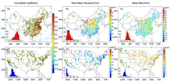
Figure 1.
Data accuracy of PM2.5 forecasts from the the European Copernicus Atmosphere Monitoring Service (CAMS) with a forecasting time horizon of 3 h (step-3) in China (a–c) and United States (US) (d–f). Dots with a black edge in (a,d) imply correlations were statistically significant at the 95% confidence interval.
Similarly, Figure 2 shows the accuracy of CAMS PM2.5 forecasts at step-120 (i.e., with a forecasting time horizon of 120 h). Noteworthy is that there is a significant decrease in data accuracy as time horizons increased from 3 to 120 h. Compared with statistical metrics shown in Figure 1 (step-3), the PM2.5 forecasts at step-120 not only showed a weaker correlation with in situ PM2.5 measurements but also suffered from larger modeling biases (only in China). This implies the degradation of forecasting accuracy as the forecasting time horizon increases. Additionally, the overestimations were significantly enlarged with the increase of forecasting time horizons, extending to cover an area of even more than half of the land areas of China. Conversely, it is interesting to notice that both RMSE and MBE were found to even decrease as time horizons increased from 3 to 120 h in CONUS. This effect is opposed to the obvious error propagation assumption that was revealed in China as the modeling biases increased significantly with the increase of forecasting time horizons.
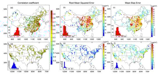
Figure 2.
Data accuracy of PM2.5 forecasts from the the European Copernicus Atmosphere Monitoring Service (CAMS) with a forecasting time horizon of 120 h (step-120) in China (a–c) and United States (US) (d–f). Dots with a black edge in (a,d) imply correlations were statistically significant at the 95% confidence interval.
To better examine the temporal evolution of data accuracy of PM2.5 forecasts, we also calculated site-specific R and RMSE between PM2.5 forecasts and co-located in situ measurements at each forecasting step. Given the evident diurnal variation in PM2.5 concentration, we adjusted the UTC time of PM2.5 forecasts to the local time (UTC+8 for China while UTC-5 for CONUS), to account for the time difference between China and US, so that the derived accuracy metrics in these two countries can be compared fairly. Figure 3 compares regional averaged R and RMSE at each forecasting time step between China and CONUS. It is indicative that the PM2.5 forecasting accuracy decreased with the increase of forecasting time horizons, especially in China, where a statistically significant decreasing trend of R and an increasing tendency of RMSE were observed. Overall, such an accuracy degradation pattern is reasonable as future PM2.5 concentration levels depend on not only the changes in emission sources but also meteorological conditions. Despite the fact that forecasting of these two factors (i.e., emission and meteorological fields) is subject to larger uncertainty, as time evolves due to the possible error propagation, we should be aware that the limited access to observational data (both meteorological data and air quality measurements) could be also a critical factor in resulting in extraordinary large biases in PM2.5 forecasts in China. This could be partially corroborated by the temporal variations in RMSE in CONUS, since no increasing trend was observed. Such an effect could be attributable to the relatively stationary variation in mean PM2.5 loading in CONUS during a short period. In other words, the CAMS forecasting model succeeded in predicting mean PM2.5 concentration levels in CONUS, but failed in capturing the fluctuations of PM2.5, which then resulted in a decreased correlation.
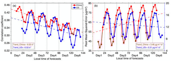
Figure 3.
Temporal variations in mean correlation coefficient (R) (a) and root mean squared error (RMSE) (b) for CAMS PM2.5 forecasts at each forecasting time step in China and US. The dashed lines in red and blue are least square lines fitted to each metric time series. Note the left axis (red) in Figure 3b refers to RMSE in China while the right axis (blue) is for the RMSE in US.
In addition to the time-evolving accuracy degradation, the forecasting accuracy was also found to vary with an evident diurnal cycle. As shown in Figure 3, the largest correlation was mainly observed at 17:00 local time in China and 16:00 in CONUS on each specific date, whereas the smallest correlation at 05:00 in China and 04:00 in CONUS. The largest RMSE was observed at 05:00 in China and 04:00 in CONUS, whereas daily minimum at 14:00 in China and 16:00 in CONUS, respectively. Such an evident diurnal variation in forecasting accuracy indicates that the current CAMS forecasting model might fail to accurately resolve the local processes, such as the variation of boundary layer height that play important roles in determining the diurnal variability of PM2.5 []. These results collectively revealed the fact that the current CAMS PM2.5 forecasts suffered from large yet nonstationary modeling biases, though detailed reasons remain unclear since numerical simulation efforts are required to diagnose the possible reasons. Nevertheless, these results highlight the importance to perform essential bias correction to account for diurnal varied large modeling biases in this PM2.5 forecasts prior to the practical usage of this dataset.
Figure 4 gives a further comparison of seasonal averaged R and RMSE to examine the possible seasonal variation in data accuracy. Evident seasonal differences were observed in the PM2.5 forecasting accuracy in both countries. In China, the highest correlation was observed in the autumn while the lowest RMSE in the summer. Given the generally low PM2.5 loading in the summer, the lowest RMSE is thus reasonable. In such context, we may conclude that the CAMS forecasting model had the highest accuracy in predicting autumntime PM2.5 concentrations in China since the RMSE in the autumn is the second lowest and the correlation is the highest. In contrast, PM2.5 forecasts in spring and winter showed a relatively low accuracy as larger biases were more likely to be observed in the spring. As indicated by the CAMS science team, the large modeling biases in these two seasons could be attributable to the newly implemented dust emission and aerosol composition schemes in the CAMS forecasting system. Specifically, the new dust emission scheme always results in high dust emission values while the newly added nitrate and ammonium compositions could lead to an overestimation of AOD. In China, dust storms occur more frequently in spring while more nitrates and ammonium are released in spring and winter due to excessive heating related primary combustions [,]. Therefore, the overestimated AOD and dust emissions may inevitably lead to significant overestimations in PM2.5 forecasts during these two seasons. On the contrary, large RMSE were more likely to be observed in summer and autumn in US, though high correlations were also observed at the meantime. More importantly, the RMSE was even found to decrease in spring and summer with the increase of forecasting time horizons, and this may help explain the decreasing trend of RMSE shown in Figure 3b, though detailed reasons remain unclear.
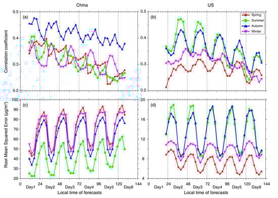
Figure 4.
Temporal evolutions of seasonal mean correlation coefficient (a,b) and RMSE (c,d) at each forecasting time step in China and US.
Figure 5 compares the regional variations in these three statistical metrics (refer to Figures S1–S2 in the Supplementary Materials for the geographic location of each region of interest). The significant variations in data accuracy across regions imply the CAMS PM2.5 forecasts failed to accurately resemble the spatial variations in PM2.5 observations, particularly in the northwest China given the lowest correlation and relatively high RMSE values. In contrast, the CAMS PM2.5 forecasts showed higher overall accuracy in predicting PM2.5 concentration in the northeast China, since it shows relatively low RMSE and MBE. Specifically, the data accuracy varied with smaller deviations along the forecasting time horizon, indicating by a shorter box as compared to others. Among the seven regions of interest, PM2.5 concentration in central China was poorly predicted given significant overestimations and large variations in the forecasting accuracy. In US, the CAMS PM2.5 forecasts poorly resembled the PM2.5 concentration in the west part of the country given much larger RMSE. Overall, the evident spatial and temporal variations in these three data accuracy metrics clearly indicate that the current CAMS PM2.5 forecasts suffered from spatially and temporally varied modeling biases.
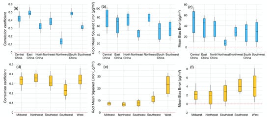
Figure 5.
Boxplots of regional averaged correlation coefficient, root mean squared error, and mean bias error at each forecasting time step in China (a–c) and United States (d–f). The black line in each box indicates the median value while the upper and bottom edges show data values at the 75% and 25% percentiles, respectively.
To examine the possible dependence of the forecasting accuracy on PM2.5 pollution levels, we also calculated correlation coefficients between regional mean PM2.5 concentration and two data accuracy metrics, namely R and RMSE in China and CONUS. As shown in Table 1, the site-specific RMSE was closely correlated with mean PM2.5 concentration levels across China except in the South China, where RMSE showed no statistical dependence (R = −0.01) on mean PM2.5 concentration values. The positive correlation between mean PM2.5 concentration levels and RMSE thus indicates the forecasted PM2.5 concentration data were subject to larger modeling biases in regions with higher PM2.5 loadings, especially over central China and the southwest of the country. In other words, the modeling biases in raw PM2.5 forecasts may resemble the spatial distribution pattern of mean PM2.5 concentration levels. Similar phenomenon was also observed in the west and southwest of CONUS as larger modeling biases may occur in regions with higher PM2.5 loadings. In contrast, there was no apparent dependence of correlation on mean PM2.5 concentration levels, except in East China, western US, where statistically significant positive correlation was observed. This implies the CAMS forecasting model can better capture the future PM2.5 concentration levels in regions with higher ambient PM2.5 loadings. The negative correlation (mid-west of US) thus means an opposite response. These dependence effects also revealed that PM2.5 forecasts derived from the current CAMS forecasting model suffered from spatially heterogeneous and magnitude dependent biases.

Table 1.
Correlation between forecasting accuracy (R and RMSE) and mean PM2.5 concentration levels across distinct regions in China and United States (US). N denotes the number of sites in each region of interest. The geographic location of each region of interest can be found in Figures S1–S2 in the Supplementary Materials.
4.2. Machine Learning-Based Calibration of CAMS PM2.5 Forecasts
Given the above revealed nonstationary and spatially heterogeneous modeling biases in CAMS PM2.5 forecasts, we proposed to reduce such biases by calibrating the original PM2.5 forecasts using a machine learning-based bias correction model. Figure 6 and Figure 7 compare the validation accuracy of CAMS PM2.5 forecasts at two specific forecasting time horizons (i.e., step-3 versus step-120) before and after the calibration. It is indicative that the data accuracy of PM2.5 forecasts was significantly improved after the calibration. In China, the R value was improved from 0.45 to 0.78 and the RMSE was reduced from 50.15 to 25.51 μg/m3 (Figure 6). This benefiting effect was even more prominent for PM2.5 forecasts at step-120, as the R value was improved from 0.43 to 0.76 and the RMSE was reduced from 91.69 to 22.79 μg/m3 (Figure 7). Similarly, the benefiting effect of the calibration method was also remarkable in US as the R value was improved from 0.39 to 0.67 (0.30 to 0.58 for step-120), while the RMSE was reduced from 15.08 to 6.53 μg/m3 (13.05 to 7.08 for step-120). In light of scatters, the calibrated data values agreed better with in situ PM2.5 measurements, though the calibrated data values still underestimated the high PM2.5 loadings to some extent.
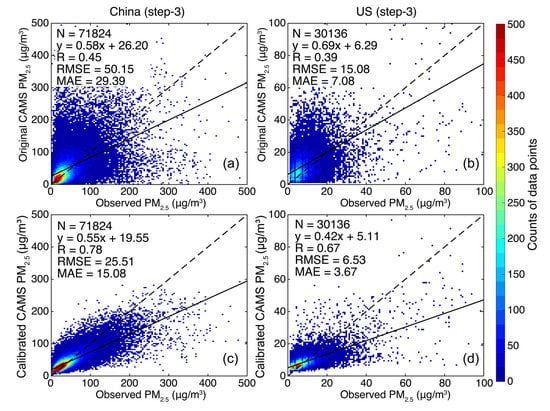
Figure 6.
Comparison of the cross-validation accuracy between the original (a,b) and the calibrated (c,d) PM2.5 forecasts with a forecasting time horizon of 3 h (step-3). Note the data values compared here were unseen data which were randomly selected and retained for the cross-validation purpose.
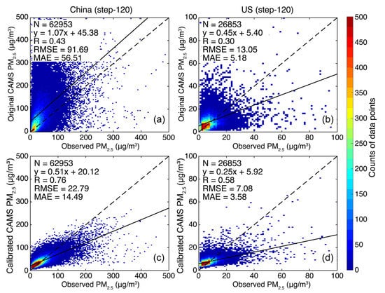
Figure 7.
Comparison of the cross-validation accuracy between the original (a,b) and the calibrated (c,d) PM2.5 forecasts with a forecasting time horizon of 120 h (step-120). Note the data values compared here were unseen data which were randomly selected and retained for the cross-validation purpose.
Figure 8 shows the site-specific data accuracy of the calibrated PM2.5 forecasts (step-3) in China and CONUS. It is indicative that the large modeling biases in raw CAMS PM2.5 forecasts were substantially reduced by the calibration model. As shown, the heterogeneous modeling biases in the original CAMS PM2.5 forecasts (Figure 1), especially the spatially varied large modeling biases in Sichuan basin and the northwest part of the country, had been significantly reduced after the calibration, resulting in a spatially more homogeneous distribution of three statistical data accuracy metrics. Figure 9 compares the improvement of mean data accuracy of PM2.5 forecasts at each forecasting time step before and after the calibration. Shown is that there was an evident improvement in the data accuracy of CAMS PM2.5 forecasts at each forecasting time step after the calibration as evidenced by improved correlation and reduced RMSE. More importantly, the diurnal varied modeling biases were also well accounted for by the calibration model. Compared with the RMSE derived from the original PM2.5 forecasts that exhibited evident diurnal variability, no apparent diurnal cycle was observed in the calibrated PM2.5 forecasts (Figure 9b). Additionally, the increasing trend of RMSE was largely reduced in the calibrated dataset. Overall, these results not only justify the effectiveness of the proposed machine learning based calibration model in reducing large modeling biases in raw CAMS PM2.5 forecasts, but also highlight the need to improve the performance of the forecasting model used in the current CAMS system. Otherwise, the nighttime PM2.5 forecasts would suffer from extraordinary large modeling biases.
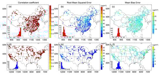
Figure 8.
Data accuracy of PM2.5 forecasts from the European Copernicus Atmosphere Monitoring Service (CAMS) with a forecasting time horizon of 3 h (step-3) in China (a–c) and United States (US) (d–f). The subplot in each figure shows the histogram of the corresponding statistical metric.
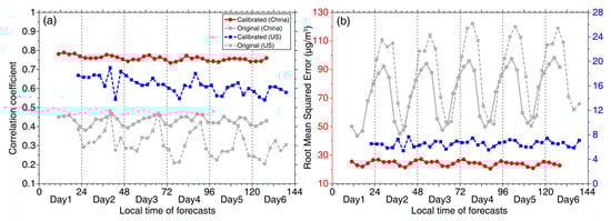
Figure 9.
Comparison of the data accuracy of PM2.5 forecasts before and after the data calibration. Note the correlation coefficient (a) and RMSE (b) compared here were derived from the cross-validation dataset. The left axis in Figure 9b (red) refers to data values of RMSE for PM2.5 forecasts in China while the right axis (blue) is for that of US.
Figure 10 and Figure 11 present a comparison of spatial distribution of PM2.5 forecasts before and after the data calibration on two different dates in different seasons in China and CONUS, respectively. The results clearly show that the large and spatially heterogeneous modeling biases in raw PM2.5 forecasts were significantly reduced after the calibration, resulting in a PM2.5 forecast better resembling the ground-based PM2.5 measurements. In spite of the effectiveness in reducing large modeling biases in raw PM2.5 forecasts, we should be aware that the calibration model is still incapable of reconstructing all PM2.5 concentration measurements (e.g., the high PM2.5 loading over the middle-to-west regions in China on 9 February 2018). This is because the calibrated data still depend highly on raw PM2.5 forecasts, as large errors in PM2.5 background fields would persist in the subsequent forecasting field without adequate corrections.
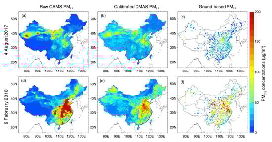
Figure 10.
Comparisons of CMAS PM2.5 forecasts with a forecasting time horizon of 3 h (step-3) before (a,d) and after (b,e) the calibration in China on two different days. (c,f) Show the in situ PM2.5 measurements on the corresponding date.
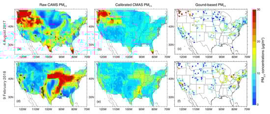
Figure 11.
Comparisons of CMAS PM2.5 forecasts with a forecasting time horizon of 3 h (step-3) before (a,d) and after (b,e) the calibration in US on two different days. (c,f) Show the in situ PM2.5 measurements on the corresponding date.
To examine the possible dependence of modeling biases, we also estimated the relative importance of predictors that were used in the random forest model to calibrate raw PM2.5 forecasts at steps 3 and 120. As shown in Figure 12, PM2.5 concentration at t0 (i.e., the initial background) was found to have the largest relative importance (RH in China), which even excess that of the raw PM2.5 forecasts at t3. This result not only emphasizes the critical role of the initial PM2.5 concentration in determining future PM2.5 concentration levels, but also implies the presence of large modeling bias in raw CAMS PM2.5 forecasts. Otherwise, the raw PM2.5 forecasts at t3 should play the most important role in resembling actual PM2.5 concentration measured at t3. Among the remaining predictors, meteorological variables such as RH and BLH as well as season are three predictors that played more important roles in calibrating PM2.5 forecasts in China. In contrast, season, P, and T were three critical predictors for the calibration of PM2.5 forecasts in US. Moreover, all meteorological variables at t0 were found to have larger importance than that of the forecast fields at t3 except RH and BLH in the US. The reasons behind this effect could be two folds. First, PM2.5 loadings vary little within a 3 h time interval. Second, the forecasted meteorological fields might suffer from large biases.
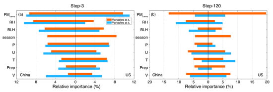
Figure 12.
Relative importance of each predictor in the random forest model to calibrate PM2.5 forecasts at steps 3 (a) and 120 (b). Variables at t0 refer to the analyzed predictors while variables at tn are forecasted fields at the nth forecasting step.
With the increase of forecasting time horizons, the relative importance of the initial PM2.5 background was reduced (Figure 12a versus Figure 12b). Rather, the forecasted PM2.5 fields were found to play the most critical role in predicting actual PM2.5 measurements. This implies the forecasted PM2.5 fields better resemble the actual PM2.5 fields, justifying the effectiveness of the CAMS forecasting model in predicting future PM2.5 pollution levels in turn. Moreover, the forecasted meteorological fields were also found to play more important roles than the analyzed fields at t0, especially in China. This is in line with expectation since the meteorological conditions may vary significantly as time horizon increases. The distinct relative importance of predictors between step-3 and step-120 indicate that both the analyzed and forecasted fields should be included to better calibrate the raw CAMS PM2.5 forecasts.
5. Discussion
In this study, we used in situ PM2.5 concentration measurements from the national air quality monitoring networks in China and US, between 2017 and 2018, as ground truth to evaluate the data accuracy of CAMS PM2.5 forecasts. Due to the coarse spatial resolution (40 km) of the model’s footprint, the CAMS PM2.5 forecasts would not perform as accurate as ground measurements and/or satellite observations on the local scale such as in urban regions. Additionally, the coarse spatial resolution could lead to significant bias in the direct point-to-grid comparisons between model outputs and ground measurements, since in situ measurements may be largely affected by pollution sources at the local scale. In other words, the assessed data accuracy could be somewhat biased given the low representation of in situ measurements, especially in regions with few monitoring stations such as western China. On the other hand, the ground-based PM2.5 data series were derived simply by averaging PM2.5 records that were measured at multiple stations falling within the same model grid cell. Such an averaging scheme is easy to apply but ignores the spatial variations in PM2.5. This is because the limited number of monitoring stations may not provide accurate pollution levels on regional scale []. In other words, the spatial representativeness of the averaged PM2.5 records could be biased, and the derived PM2.5 records might poorly represent PM2.5 concentration levels on the given CAMS grid cell. In such context, the reported data accuracy could be prone to large uncertainty. Meanwhile, the spatial distribution and/or density of monitoring stations is also a critical factor that could influence the representativeness of the averaged PM2.5 record []. For instance, same number of PM2.5 records with the one measured all in downtown areas, while the other sampled in both rural and urban regions may result in two distinct PM2.5 concentration levels if we simply averaged each set of records. Overall, the scales related bias should be recognized in interpreting point-to-grid comparison results, especially even at a much coarse model grid resolution.
In regard to the temporal evolution of R, RMSE, and MBE, we observed that the forecasting accuracy generally decreased with the increase of forecasting time horizons. This is in line with expectation since the forecasted PM2.5 fields would suffer from larger bias due to error propagation and larger uncertainty in the forecasted meteorological fields. However, noteworthy is that there was no significant increase in RMSE in US with the extending of forecasting time horizons, the exact reason remains unclear and this is more likely to be associated with the near stationary variability of daily mean PM2.5 concentration levels in US. Moreover, an evident diurnal cycle was observed in these statistical metrics (Figure 3 and Figure 4), indicating the presence of diurnal varied biases in the CAMS forecasted PM2.5 fields. Such a diurnal variation pattern was also found by Marécal et al. when evaluating the performance of models used in the European regional air quality system of MACC []. Since CAMS was a heritage of the MACC project, similar diurnal varied modeling bias revealed in the current CAMS PM2.5 forecasts implies that the CAMS model still fails to account for the diurnal varied modeling bias found in the MACC project. In such context, we may ascribe the observed diurnal varied bias to the defects of CAMS model in which factors modulating the diurnal variability of PM2.5, like variations in emissions and boundary layer height might be not well resolved [].
To further improve the accuracy of CAMS PM2.5 forecasts, a calibration model was hereby developed by using the random forest method to account for large modeling biases in raw CAMS PM2.5 forecasts. Such a data-driven method was proven to be effective in reducing nonlinear and nonstationary modeling biases in CAMS PM2.5 forecasts by making use of both analyzed and forecasted PM2.5 and meteorological fields, rendering the calibrated PM2.5 forecasts higher accuracy in resembling ground PM2.5 measurements. Nevertheless, we should notice that only the analyzed and forecasted meteorological fields were used other than PM2.5 data whereas factors indicating the actual aerosol loading (e.g., satellite AOD observations) were not included. The absence of observational aerosol data made the developed calibration model might be incapable of correcting large modeling biases in regions with high PM2.5 loadings due to large bias in the analyzed PM2.5 field. To derive better PM2.5 forecasts and/or to account for spatially and temporally varied large modeling biases in CAMS PM2.5 concentration forecasts, more accurate aerosol observational data and auxiliary factors that are closely related to the production and dispersion of PM2.5 particles (e.g., hourly boundary layer height) could be included.
6. Conclusions
In this study, the data accuracy of CAMS PM2.5 forecasts was evaluated using two-year hourly in situ PM2.5 concentration measurements that were sampled from the national air quality monitoring network in China and CONUS. The ground-based validation results revealed a relatively low accuracy of the raw CAMS PM2.5 forecasts given the presence of nonlinear and nonstationary modeling biases. Temporally, the data accuracy of PM2.5 forecasts generally decreased with the increase of forecasting time horizons. Additionally, the data accuracy was found to vary with evident diurnal cycle as the highest accuracy was more likely to be observed in the late afternoon (17:00 local time in China and 16:00 in CONUS), whereas the lowest accuracy in the early morning (05:00 local time in China and 04:00 in CONUS). Moreover, the data accuracy varied between seasons as PM2.5 forecasts in the autumn in China (spring in US) appeared to be better simulated. Generally, the revealed low accuracy of the raw CAMS PM2.5 forecasts could be attributable to factors such as the coarse spatial resolution of CAMS model, representation errors due to distinct scales of ground measurements and model outputs, limited access to observational data, as well as improper formulation of boundary layer effect in the CAMS model. A machine learning-based data calibration model was then developed to reduce large modeling biases that were found in the raw CAMS PM2.5 forecasts. The validation results indicate that the calibrated data not only had a much lower RMSE but better correlated with ground-based PM2.5 measurements, suggesting an improved accuracy of the calibrated PM2.5 forecasts. Overall, the assessed data accuracy of CAMS PM2.5 forecasts in this study provides a good reference to potential data users, and the developed machine learning-based calibration model can be used as a promising postprocessing measures to improve the data accuracy.
Supplementary Materials
The following are available online at https://www.mdpi.com/2072-4292/12/22/3813/s1, Figure S1: The map of seven geographic divisions in China, Figure S2: The map of five major geographic divisions in the United States.
Author Contributions
Conceptualization, K.B.; methodology, C.W., K.L. and K.B.; validation: C.W., K.L. and K.B.; data curation: W.C. and K.L.; formal analysis, W.C., K.L. and K.B.; writing—original draft preparation, W.C.; writing—review and editing, K.B.; visualization, W.C.; supervision, K.B.; project administration, K.B.; funding acquisition, K.B. All authors have read and agreed to the published version of the manuscript.
Funding
This study was supported by the National Natural Science Foundation of China (Grant numbers 41701413) and the Shanghai Committee of Science and Technology (Grant No. 20ZR1415900).
Acknowledgments
We are grateful to three anonymous reviewers for their copious and insightful comments in helping improve the quality of this manuscript. Ground-based PM2.5 concentration measurements in China and the United States were collected from the China National Environment Monitoring Centre (http://www.cnemc.cn) and the Environmental Protection Agency of United States (https://www.epa.gov/environmental-topics), respectively. The CAMS PM2.5 forecast data were download from the European Centre for Medium-Range Weather Forecasts (https://apps.ecmwf.int/datasets/data/cams-nrealtime/levtype=sfc/).
Conflicts of Interest
The authors declare no conflict of interest.
References
- Silver, B.; Reddington, C.L.; Arnold, S.R.; Spracklen, D.V. Substantial changes in air pollution across China during 2015–2017. Environ. Res. Lett. 2018, 13. [Google Scholar] [CrossRef]
- West, J.J.; Cohen, A.; Dentener, F.; Brunekreef, B.; Zhu, T.; Armstrong, B.; Bell, M.L.; Brauer, M.; Carmichael, G.; Costa, D.L.; et al. What We Breathe Impacts Our Health: Improving Understanding of the Link between Air Pollution and Health. Environ. Sci. Technol. 2016, 50, 4895–4904. [Google Scholar] [CrossRef] [PubMed]
- Jerrett, M. The death toll from air-pollution sources. Nature 2015, 525, 330–331. [Google Scholar] [CrossRef] [PubMed]
- Lelieveld, J.; Evans, J.S.; Fnais, M.; Giannadaki, D.; Pozzer, A. The contribution of outdoor air pollution sources to premature mortality on a global scale. Nature 2015, 525, 367–371. [Google Scholar] [CrossRef] [PubMed]
- Pope, C.A.; Ezzati, M.; Dockery, D.W. Fine-particulate air pollution and life expectancy in the United States. N. Engl. J. Med. 2009, 360, 376–386. [Google Scholar] [CrossRef]
- Zhang, Q.; He, K.; Hong, H. Cleaning China’s air. Nature 2012, 484, 161–162. [Google Scholar] [CrossRef]
- Hadley, M.B.; Vedanthan, R.; Fuster, V. Air pollution and cardiovascular disease: A window of opportunity. Nat. Rev. Cardiol. 2019, 15, 193–194. [Google Scholar] [CrossRef]
- Bond, T.C.; Doherty, S.J.; Fahey, D.W.; Forster, P.M.; Berntsen, T.; Deangelo, B.J.; Flanner, M.G.; Ghan, S.; Kärcher, B.; Koch, D.; et al. Bounding the role of black carbon in the climate system: A scientific assessment. J. Geophys. Res. Atmos. 2013, 118, 5380–5552. [Google Scholar] [CrossRef]
- Charlson, R.J.; Schwartz, S.E.; Hales, J.M.; Cess, R.D.; Coakley, J.A.; Hansen, J.E.; Hofmann, D.J. Climate forcing by anthropogenic aerosols. Science 1992, 255, 423–430. [Google Scholar] [CrossRef]
- Hansen, J.; Sato, M.; Ruedy, R.; Nazarenko, L.; Lacis, A.; Schmidt, G.A.; Russell, G.; Aleinov, I.; Bauer, M.; Bauer, S.; et al. Efficacy of climate forcings. J. Geophys. Res. D Atmos. 2005, 110, 1–45. [Google Scholar] [CrossRef]
- Tie, X.; Madronich, S.; Walters, S.; Edwards, D.P.; Ginoux, P.; Mahowald, N.; Zhang, R.Y.; Lou, C.; Brasseur, G. Assessment of the global impact of aerosols on tropospheric oxidants. J. Geophys. Res. Atmos. 2005, 110, 1–32. [Google Scholar] [CrossRef]
- Becker, J.M.; Merrifield, M.A.; Yoon, H. Infragravity waves on fringing reefs in the tropical Pacific: Dynamic setup. J. Geophys. Res. Ocean. 2016, 121, 3010–3028. [Google Scholar] [CrossRef]
- Bai, K.; Ma, M.; Chang, N.-B.; Gao, W. Spatiotemporal trend analysis for fine particulate matter concentrations in China using high-resolution satellite-derived and ground-measured PM2.5 data. J. Environ. Manag. 2019, 233, 530–542. [Google Scholar] [CrossRef] [PubMed]
- Shen, F.; Zhang, L.; Jiang, L.; Tang, M.; Gai, X.; Chen, M.; Ge, X. Temporal variations of six ambient criteria air pollutants from 2015 to 2018, their spatial distributions, health risks and relationships with socioeconomic factors during 2018 in China. Environ. Int. 2020, 137, 105556. [Google Scholar] [CrossRef]
- Xiao, Q.; Wang, Y.; Chang, H.H.; Meng, X.; Geng, G.; Lyapustin, A.; Liu, Y. Full-coverage high-resolution daily PM2.5 estimation using MAIAC AOD in the Yangtze River Delta of China. Remote Sens. Environ. 2017, 199, 437–446. [Google Scholar] [CrossRef]
- Rodriguez, D.; Valari, M.; Payan, S.; Eymard, L. On the spatial representativeness of NOX and PM10 monitoring-sites in Paris, France. Atmos. Environ. X 2019, 1, 100010. [Google Scholar] [CrossRef]
- Shi, X.; Zhao, C.; Jiang, J.H.; Wang, C.; Yang, X.; Yung, Y.L. Spatial representativeness of PM2.5 concentrations obtained using observations from network stations. J. Geophys. Res. Atmos. 2018, 123, 3145–3158. [Google Scholar] [CrossRef]
- Zhang, Y.; Li, Z. Remote sensing of atmospheric fine particulate matter (PM2.5) mass concentration near the ground from satellite observation. Remote Sens. Environ. 2015, 160, 252–262. [Google Scholar] [CrossRef]
- Gupta, P.; Christopher, S.A.; Wang, J.; Gehrig, R.; Lee, Y.; Kumar, N. Satellite remote sensing of particulate matter and air quality assessment over global cities. Atmos. Environ. 2006, 40, 5880–5892. [Google Scholar] [CrossRef]
- Shen, H.; Li, T.; Yuan, Q.; Zhang, L. Estimating regional ground-level PM2.5 directly from satellite top-of-atmosphere reflectance using deep belief networks. J. Geophys. Res. Atmos. 2018, 123, 13875–13886. [Google Scholar] [CrossRef]
- van Donkelaar, A.; Martin, R.V.; Spurr, R.J.D.; Drury, E.; Remer, L.A.; Levy, R.C.; Wang, J. Optimal estimation for global ground-level fine particulate matter concentrations. J. Geophys. Res. Atmos. 2013, 118, 5621–5636. [Google Scholar] [CrossRef]
- Levy, R.C.; Mattoo, S.; Munchak, L.A.; Remer, L.A.; Sayer, A.M.; Patadia, F.; Hsu, N.C. The Collection 6 MODIS aerosol products over land and ocean. Atmos. Meas. Tech. 2013, 6, 2989–3034. [Google Scholar] [CrossRef]
- Wei, J.; Li, Z.; Peng, Y.; Sun, L. MODIS Collection 6.1 aerosol optical depth products over land and ocean: Validation and comparison. Atmos. Environ. 2019, 201, 428–440. [Google Scholar] [CrossRef]
- Garay, M.J.; Witek, M.L.; Kahn, R.A.; Seidel, F.C.; Limbacher, J.A.; Bull, M.A.; Diner, D.J.; Hansen, E.G.E.G.; Kalashnikova, O.V.; Lee, H.; et al. Introducing the 4.4km spatial resolution Multi-Angle Imaging SpectroRadiometer (MISR) aerosol product. Atmos. Meas. Tech. 2020, 13, 593–628. [Google Scholar] [CrossRef]
- Engel-Cox, J.; Kim Oanh, N.T.; van Donkelaar, A.; Martin, R.V.; Zell, E. Toward the next generation of air quality monitoring: Particulate Matter. Atmos. Environ. 2013, 80, 584–590. [Google Scholar] [CrossRef]
- Guo, J.; Xia, F.; Zhang, Y.; Liu, H.; Li, J.; Lou, M.; He, J.; Yan, Y.; Wang, F.; Min, M.; et al. Impact of diurnal variability and meteorological factors on the PM2.5—AOD relationship: Implications for PM2.5 remote sensing. Environ. Pollut. 2017, 221, 94–104. [Google Scholar] [CrossRef]
- Lee, H.J.; Liu, Y.; Coull, B.A.; Schwartz, J.; Koutrakis, P. A novel calibration approach of MODIS AOD data to predict PM2.5 concentrations. Atmos. Chem. Phys. 2011, 11, 7991–8002. [Google Scholar] [CrossRef]
- Yang, Q.; Yuan, Q.; Yue, L.; Li, T.; Shen, H.; Zhang, L. The relationships between PM2.5 and aerosol optical depth (AOD) in mainland China: About and behind the spatio-temporal variations. Environ. Pollut. 2019, 248, 526–535. [Google Scholar] [CrossRef]
- Reid, C.E.; Jerrett, M.; Petersen, M.L.; Pfister, G.G.; Morefield, P.E.; Tager, I.B.; Raffuse, S.M.; Balmes, J.R. Spatiotemporal prediction of fine particulate matter during the 2008 Northern California wildfires using machine learning. Environ. Sci. Technol. 2015, 49, 3887–3896. [Google Scholar] [CrossRef]
- Wang, M.; Sampson, P.D.; Hu, J.; Kleeman, M.; Keller, J.P.; Olives, C.; Szpiro, A.A.; Vedal, S.; Kaufman, J.D. Combining land-use regression and chemical transport modeling in a spatiotemporal geostatistical model for ozone and PM2.5. Environ. Sci. Technol. 2016, 50, 5111–5118. [Google Scholar] [CrossRef]
- Liu, H.; Yan, R.; Yang, J. Credibility and statistical characteristics of CAMSRA and MERRA-2 AOD reanalysis products over the Sichuan Basin during 2003–2018. Atmos. Environ. 2021, 244, 117980. [Google Scholar] [CrossRef]
- Varga-Balogh, A. Time-dependent downscaling of PM2.5 predictions from CAMS air quality models to urban monitoring sites in Budapest. Atmosphere 2020, 11, 669. [Google Scholar] [CrossRef]
- Zhang, T.; Zang, L.; Mao, F.; Wan, Y.; Zhu, Y. Evaluation of Himawari-8/AHI, MERRA-2, and CAMS aerosol products over China. Remote Sens. 2020, 12, 1684. [Google Scholar] [CrossRef]
- Hua, Z.; Sun, W.; Yang, G.; Du, Q. A full-coverage daily average PM2.5 retrieval method with two-stage IVW fused MODIS C6 AOD and two-stage GAM model. Remote Sens. 2019, 11, 1558. [Google Scholar] [CrossRef]
- Liang, F.; Xiao, Q.; Wang, Y.; Lyapustin, A.; Li, G.; Gu, D.; Pan, X.; Liu, Y. MAIAC-based long-term spatiotemporal trends of PM2.5 in Beijing, China. Sci. Total Environ. 2018, 616–617, 1589–1598. [Google Scholar] [CrossRef] [PubMed]
- Yang, M.; Fan, H.; Zhao, K. PM2.5 prediction with a novel multi-step-ahead forecasting model based on dynamic wind field distance. Int. J. Environ. Res. Public Health 2019, 16, 4482. [Google Scholar] [CrossRef] [PubMed]
- Mao, X.; Shen, T.; Feng, X. Prediction of hourly ground-level PM2.5 concentrations 3 days in advance using neural networks with satellite data in eastern China. Atmos. Pollut. Res. 2017, 8, 1005–1015. [Google Scholar] [CrossRef]
- Qi, Y.; Li, Q.; Karimian, H.; Liu, D. A hybrid model for spatiotemporal forecasting of PM2.5 based on graph convolutional neural network and long short-term memory. Sci. Total Environ. 2019, 664, 1–10. [Google Scholar] [CrossRef]
- Morcrette, J.J.; Boucher, O.; Jones, L.; Salmond, D.; Bechtold, P.; Beljaars, A.; Benedetti, A.; Bonet, A.; Kaiser, J.W.; Razinger, M.; et al. Aerosol analysis and forecast in the european centre for medium-range weather forecasts integrated forecast system: Forward modeling. J. Geophys. Res. Atmos. 2009, 114, 1–17. [Google Scholar] [CrossRef]
- Benedetti, A.; Morcrette, J.; Boucher, O.; Dethof, A.; Engelen, R.J.; Fisher, M.; Flentjes, H.; Huneeus, N.; Jones, L.; Kaiser, J.W.; et al. Aerosol Analysis and Forecast in the ECMWF Integrated Forecast System: Data Assimilation; ECMWF: Reading, UK, 2008; pp. 1–23. [Google Scholar]
- Atmosphere, C.; Service, M. Validation Report of the CAMS Near-Real Time Global Atmospheric Composition Service. Available online: http://atmosphere.copernicus.eu/sites/default/files/201903/16_CAMS84_2018SC1_D1.1.1_SON2018_v1.pdf (accessed on 20 August 2020).
- Validation of the Copernicus Atmosphere Monitoring Service (CAMS). Available online: https://www.knmi.nl/research/satellite-measurements/projects/validation-of-the-copernicus-atmosphere-monitoring-service-cams (accessed on 26 August 2020).
- Wang, Y.; Chen, H.; Wu, Q.; Chen, X.; Wang, H.; Gbaguidi, A.; Wang, W.; Wang, Z. Three-year, 5 km resolution China PM2.5 simulation: Model performance evaluation. Atmos. Res. 2018, 207, 1–13. [Google Scholar] [CrossRef]
- Bai, L.; Wang, J.; Ma, X.; Lu, H. Air pollution forecasts: An overview. Int. J. Environ. Res. Public Health 2018, 15, 780. [Google Scholar] [CrossRef] [PubMed]
- Feng, X.; Li, Q.; Zhu, Y.; Hou, J.; Jin, L.; Wang, J. Artificial neural networks forecasting of PM2.5 pollution using air mass trajectory based geographic model and wavelet transformation. Atmos. Environ. 2015, 107, 118–128. [Google Scholar] [CrossRef]
- Bai, K.; Chang, N.-B.; Yu, H.; Gao, W. Statistical bias correction for creating coherent total ozone record from OMI and OMPS observations. Remote Sens. Environ. 2016, 182, 150–168. [Google Scholar] [CrossRef]
- Ahmed, K.F.; Wang, G.; Silander, J.; Wilson, A.M.; Allen, J.M.; Horton, R.; Anyah, R. Statistical downscaling and bias correction of climate model outputs for climate change impact assessment in the U.S. northeast. Glob. Planet. Chang. 2013, 100, 320–332. [Google Scholar] [CrossRef]
- Amengual, A.; Homar, V.; Romero, R.; Alonso, S.; Ramis, C. A statistical adjustment of regional climate model outputs to local scales: Application to Platja de Palma, Spain. J. Clim. 2012, 25, 939–957. [Google Scholar] [CrossRef]
- Singh, M.K.; Gautam, R.; Venkatachalam, P. Bayesian merging of MISR and MODIS aerosol. IEEE J. Sel. Top. Appl. EARTH Obs. Remote Sens. 2017, 10, 5186–5200. [Google Scholar] [CrossRef]
- Wang, Y.; Yuan, Q.; Li, T.; Shen, H.; Zheng, L.; Zhang, L. Large-scale MODIS AOD products recovery: Spatial-temporal hybrid fusion considering aerosol variation mitigation. ISPRS J. Photogramm. Remote Sens. 2019, 157, 1–12. [Google Scholar] [CrossRef]
- Jiang, T.; Chen, B.; Chan, K.K.Y.; Xu, B. Himawari-8/AHI and MODIS aerosol optical depths in China: Evaluation and comparison. Remote Sens. 2019, 11, 1011. [Google Scholar] [CrossRef]
- Wei, J.; Li, Z.; Cribb, M.; Huang, W.; Xue, W.; Sun, L.; Guo, J.; Peng, Y.; Li, J.; Lyapustin, A.; et al. Improved 1 km resolution PM2.5 estimates across China using enhanced space-time extremely randomized trees. Atmos. Chem. Phys. 2020, 20, 3273–3289. [Google Scholar] [CrossRef]
- Jiang, T.; Chen, B.; Nie, Z.; Ren, Z.; Xu, B.; Tang, S. Estimation of hourly full-coverage PM2.5 concentrations at 1-km resolution in China using a two-stage random forest model. Atmos. Res. 2021, 248, 105146. [Google Scholar] [CrossRef]
- Li, L.; Franklin, M.; Girguis, M.; Lurmann, F.; Wu, J.; Pavlovic, N.; Breton, C.; Gilliland, F.; Habre, R. Spatiotemporal imputation of MAIAC AOD using deep learning with downscaling. Remote Sens. Environ. 2020, 237, 111584. [Google Scholar] [CrossRef] [PubMed]
- Bai, K.; Li, K.; Guo, J.; Yang, Y.; Chang, N.-B. Filling the gaps of in situ hourly PM2.5 concentration data with the aid of empirical orthogonal function analysis constrained by diurnal cycles. Atmos. Meas. Tech. 2020, 13, 1213–1226. [Google Scholar] [CrossRef]
- Bai, K.; Li, K.; Chang, N.-B.; Gao, W. Advancing the prediction accuracy of satellite-based PM2.5 concentration mapping: A perspective of data mining through in situ PM2.5 measurements. Environ. Pollut. 2019, 254, 113047. [Google Scholar] [CrossRef]
- Wei, J.; Huang, W.; Li, Z.; Xue, W.; Peng, Y.; Sun, L.; Cribb, M. Estimating 1-km-resolution PM2.5 concentrations across China using the space-time random forest approach. Remote Sens. Environ. 2019, 231, 111221. [Google Scholar] [CrossRef]
- Al, B.E.T. Calibration of machine learning-based probabilistic hail predictions for operational forecasting. Weather Forecast. 2020, 35, 149–168. [Google Scholar] [CrossRef]
- Kingdom, U. Probabilistic forecast calibration using ECMWF and GFS ensemble reforecasts. Part I: Two-meter temperatures. Mon. Weather Rev. 2007, 136, 2608–2619. [Google Scholar] [CrossRef]
- Kingdom, U. Probabilistic forecast calibration using ECMWF and GFS ensemble reforecasts. Part II: Precipitation. Mon. Weather Rev. 2008, 136, 2620–2632. [Google Scholar] [CrossRef]
- Liu, Y.; Cao, G.; Zhao, N. Integrate machine learning and geostatistics for high-resolution mapping of ground-level PM2.5 concentrations. In Spatiotemporal Analysis of Air Pollution and Its Application in Public Health; Elsevier: Amsterdam, The Netherlands, 2020; pp. 135–151. [Google Scholar]
- Manning, M.I.; Martin, R.V.; Hasenkopf, C.; Flasher, J.; Li, C. Diurnal patterns in global fine particulate matter concentration. Environ. Sci. Technol. Lett. 2018, 5, 687–691. [Google Scholar] [CrossRef]
- Deng, H.; Jiang, W.-F.; Chen, Y.-Y.; Shu, S.-G. The temporal and spatial distribution of dust storms on the North China Plain, AD 1464-1913. Holocene 2013, 23, 625–634. [Google Scholar] [CrossRef]
- Guan, Q.; Sun, X.; Yang, J.; Pan, B.; Zhao, S.; Wang, L. Dust storms in northern China: Long-term spatiotemporal characteristics and climate controls. J. Clim. 2017, 30, 6683–6700. [Google Scholar] [CrossRef]
- Loew, A.; Bell, W.; Brocca, L.; Bulgin, C.E.; Burdanowitz, J.; Kinzel, J.; Klepp, C.; Lambert, J.; Schaepman-strub, G. Validation practices for satellite-based Earth observation data across communities. Rev. Geophys. 2017, 55, 779–817. [Google Scholar] [CrossRef]
- Marécal, V.; Peuch, V.H.; Andersson, C.; Andersson, S.; Arteta, J.; Beekmann, M.; Benedictow, A.; Bergström, R.; Bessagnet, B.; Cansado, A.; et al. A regional air quality forecasting system over Europe: The MACC-II daily ensemble production. Geosci. Model Dev. 2015, 8, 2777–2813. [Google Scholar] [CrossRef]
Publisher’s Note: MDPI stays neutral with regard to jurisdictional claims in published maps and institutional affiliations. |
© 2020 by the authors. Licensee MDPI, Basel, Switzerland. This article is an open access article distributed under the terms and conditions of the Creative Commons Attribution (CC BY) license (http://creativecommons.org/licenses/by/4.0/).