Investigating the Error Propagation from Satellite-Based Input Precipitation to Output Water Quality Indicators Simulated by a Hydrologic Model

Abstract

This study investigated the propagation of errors in input satellite-based precipitation products (SPPs) on streamflow and water quality indicators simulated by a hydrological model in the Occoquan Watershed, located in the suburban Washington, D.C. area. A dense rain gauge network was used as reference to evaluate three SPPs which are based on different retrieval algorithms. A Hydrologic Simulation Program-FORTRAN (HSPF) hydrology and water quality model was forced with the three SPPs to simulate output of streamflow (Q), total suspended solids (TSS), stream temperature (TW), and dissolved oxygen (DO). Results indicate that the HSPF model may have a dampening effect on the precipitation-to-streamflow error. The bias error propagation of all three SPPs showed a positive dependency on basin scale for streamflow and TSS, but not for TW and DO. On a seasonal basis, bias error propagation varied by product, with larger values generally found in fall and winter. This study demonstrated that the spatiotemporal variability of SPPs, along with their algorithms to estimate precipitation, have an influence on water quality simulations in a hydrologic model.

1. Introduction

It is well understood that precipitation is the most important forcing input in a hydrologic model, as it influences both watershed hydrology and water quality processes. Land surface and hydrologic models are greatly influenced by the accuracy of input precipitation data including its spatial and temporal distribution, intensity, and duration [1,2,3]. While the traditional approach has been to measure precipitation using ground-based rain gauges, the use of satellite-based precipitation products (SPPs) in hydrologic modeling has been gaining more popularity due to their continuous geographic coverage with high spatial and temporal resolution. Whilst these products offer a viable resource, seasonal precipitation patterns, storm type, resolution of measurement, and background surface, all have an influence on the performance of SPPs and thus impact the output of hydrologic models [4,5]. Major sources of uncertainty with SPPs emerge from the inaccuracy of instrumentation, sampling errors, and algorithmic miscalculations [6]. In addition to errors associated with precipitation input, uncertainty in hydrologic modeling may come from a number of other sources such as input parameter heterogeneity, model structure and algorithm errors, and boundary condition errors. Relevant literature to this study addressed herein includes: (1) SPP uncertainty associated with hydrologic modeling, (2) propagation of error from precipitation to streamflow simulated by a hydrologic model, and (3) precipitation product resolution impact on water quality simulation error.

Understanding the uncertainty associated with individual SPPs is crucial when assessing their performance as input into a hydrologic model. SPPs combine information mainly from geostationary infrared (IR) and/or low-orbiting passive microwave (PMW) satellites. Many studies have documented the performance of SPPs, suggesting that seasonal patterns and types of precipitation can impact the quality of the retrieval. For instance, thermal IR algorithms may miss light stratiform precipitation events and snow cover [4,7]. Ebert et al. [8] reported that in temperate climates, SPPs generally perform better with convective storms during the warm season and that IR-based SPPs decline in accuracy with stratiform precipitation. Conversely, PMW algorithms may underestimate heavy precipitation events often associated with convective storms. Similarly, Li et al. [9] evaluated TMPA 3B42 and PERSIANN, PMW- and IR-based algorithms, respectively, over the Poyang Lake basin in China and found that both TMPA and PERSIANN underestimated rainfall in comparison to rain gauges and both SPPs had a dependence on elevation.

Numerous past studies have discussed how to quantify the uncertainty of SPPs and the relationship between forcing precipitation estimated by SPPs and their simulated streamflow results through a hydrologic model [10,11,12,13,14,15,16,17,18,19,20,21]. Results documented that output simulations derived from SPPs can be affected by event intensity, product resolution, seasonal performance, and basin scale, noting that moderate precipitation magnitudes, larger domain scales, longer time integration, and finer spatial and temporal resolutions of SPPs generally improve the accuracy in simulating streamflow [4,20,22,23,24]. Furthermore, in a recent study by Satgé et al. [25], 12 SPPs were evaluated in the Lake Titicaca region of South America for space–time accuracy and consistency reproduced through a hydrological model. Satgé et al. [25] found SPPs varied significantly when used to reproduce gauge estimates and streamflow observations depending on the time window considered, underlying the importance of strategically considering the space–time consistency of SPPs for use in hydrologic models. Satellite data have also been used in a number of other hydrological applications such as land cover acquisition [26] and estimating groundwater levels [27].

Several studies have also examined the propagation of error from SPPs to streamflow, indicating that the output error is highly dependent on the uncertainty associated with the forcing precipitation dataset. Errors generated from SPP resolution, both spatial and temporal, are known to have a significant impact on the error in streamflow. Nijssen and Lettenmaier [6], Flack et al. [10], Hossain and Anagnostou [11], Maggioni et al. [15], Mei et al. [16], Nikolopoulos et al. [17], Seyyedi et al. [18], Yu et al. [19], Zhang et al. [21], Yang et al. [24], Guetter and Georgakakos [28], Vivoni et al. [29], and others all found that errors associated with precipitation input can have an amplifying transformation on simulated streamflow uncertainty with relative errors magnified up to three times greater than input errors. Maggioni et al. [15] reported that error metrics of ensemble precipitation for three SPPs in the Tar-Pamlico basin in the southeast United States (U.S.) had no dependency on basin scale for relative bias, although relative root mean square error (rRMSE) decreased as a function of scale. Their results also showed that biases doubled, while RMSE decreased as a function of basin scale between input and output simulations. Vergara et al. [30] also reported an amplified bias and a dampened RMSE in the same basin. Another study investigated error corrections to SPPs in streamflow simulations through an ensemble error model in the Tocantins-Arguaia basin, Brazil [10]. Results there indicated that mean errors and RMSEs decreased as a function of basin scale, but no scale dependence on the precipitation-to-streamflow error propagation was observed. Yu et al. [19] quantified the uncertainty propagation of rainfall forecasts into streamflow through a distributed hydrologic model in the Kii Peninsula of Japan. Their results coincided with prior studies demonstrating a decrease in uncertainty by basin scale. Ehsan Bhuiyan et al. [31] investigated the propagation of precipitation uncertainty to simulated surface runoff, subsurface runoff, and evapotranspiration in the Iberian Peninsula using five SPPs, showing that uncertainties in modeled surface runoff were strongly sensitive to precipitation uncertainty. Hostache et al. [32] studied errors propagated through a hydrologic model in the Alzette River basin, Luxembourg, and found that understanding errors associated with input precipitation is vital to evaluating error-associated river flow forecasts. In addition to basin scale, other factors have been cited to impact the error propagation of streamflow including complex terrain and elevation [16,17], hydrologic model type and complexity [32,33], and seasonality [16,29,34].

Research associated with the use of satellite and reanalysis precipitation products for water quality modeling is very limited. Neal et al. [35] found that soil water chemistry has variability at the local scale, translating into a range of responses in the chemistry of localized runoff, and thus streamflow, further indicating that a high temporal frequency and spatial resolution is needed for modeling and simulating streamflow processes including TSS in the River Severn basin, United Kingdom. Himanshu et al. [36] evaluated the performance of TMPA 3B42V7 for predicting suspended sediment loads in two watersheds in South India using a machine learning technique and found moderate prediction efficiency. Stryker et al. [37] used the North American Regional Reanalysis data for simulating suspended sediment loads and concentrations in the Mad River watershed located in Vermont, U.S.; however, the main objective of this study was to evaluate model performance for sediment simulations as opposed to the uncertainty of precipitation inputs. A recent study by Ma et al. [38] investigated the use of two SPPs and one reanalysis product in the Lancang River basin in Southwest China to assess their performance in simulating streamflow and suspended sediment using the Soil and Water Assessment Tool (SWAT) model. They found that, at the monthly timestep, both SPPs were better at estimating precipitation than the reanalysis product and also both SPPs had a good capability of modeling monthly streamflow and sediment loads. While this study evaluated spatial and temporal sediment yield, it neither considered the spatial and temporal variability of SPPs nor evaluated the propagation of uncertainty between precipitation input and model output. Furthermore, while there is substantial research investigating the association between precipitation and water quality response (e.g., [35,39,40,41,42,43,44,45,46,47]), only a few studies investigated how the spatial and temporal differences of SPPs may impact the simulation and forecasting of water quality [38,48]. Initial research conducted by Solakian et al. [48] showed that spatial and temporal differences in SPP resolutions, along with the algorithms used to estimate precipitation magnitude, had an impact on modeled streamflow and water quality indicators in the Occoquan Watershed, Virginia, U.S. It was also noted that the seasonality dissimilarities observed in SPPs may translate into seasonal differences in simulated streamflow and water quality indicators. However, the Solakian et al. [48] study did not evaluate the seasonal performance of SPPs, or seasonal model response, nor did it examine the propagation of error between model input precipitation data and model simulation output.

This work assesses the propagation of errors from input precipitation using SPPs (at different resolutions) to water quality indicator output simulated through a hydrologic model by answering the following research questions that have never been addressed in previous work: (1) How well do SPPs perform seasonally compared to rain gauges in the Occoquan Watershed? (2) How well do SPPs perform in simulating streamflow and water quality indicators, both temporally (seasonally) and spatially (by basin scale)? (3) How does the performance of SPPs influence the propagation of error between input precipitation and simulated streamflow and water quality indicator output? This study builds upon the previous work of Solakian et al. (2019) and others, providing a comprehensive evaluation of the seasonal skill of three different SPPs and the propagation of error simulated through a hydrologic model. To accomplish this, SPPs of varying native spatial and temporal resolutions are compared against observations from a dense rain gauge network over the Occoquan Watershed. The three SPPs evaluated in this study are used as forcing input into a gauge-calibrated hydrologic and water quality model to simulate streamflow and three water quality indicators (i.e., total suspended solids, stream water temperature, and dissolved oxygen) at six locations within the watershed. The skill of the SPP-based model simulations is then compared to gauge-based simulations over a five-year study period (2008–2012). The propagation of error from input precipitation to simulated output for each of the three products is investigated by basin scale and on a seasonal basis. Section 2 presents the study area, the datasets, and the hydrologic model used in this study. Section 2 also illustrates the methods employed in this analysis to assess the uncertainty of SPPs, simulated output, and the propagation of error. Section 3 interprets the results of this study, while Section 4 discusses the results. Section 5 provides conclusory remarks of notable findings.

2. Materials and Methods

2.1. Study Area

The Occoquan Watershed is a tributary of the Potomac River, which discharges into the Chesapeake Bay, a body of water that has been a major focus of scientific studies and environmental restoration efforts since the 1980s to combat pollution discharged from the watershed and the presence of aquatic dead zones in the bay [49]. The Occoquan Watershed is located in the metropolitan area of Washington, DC, USA, and is approximately 1500 km² in size with two main run-of-the-river water reservoirs: Lake Manassas and the Occoquan Reservoir. The watershed is characterized by a mix of urban and suburban land use with a mild topographic variation. For over 40 years, the watershed has been monitored by a network of rain gauges and stream monitoring stations. The watershed contributes in part to the drinking water supply of residents in the area (on average, 40% of the annual demand for almost two million people), yet has experienced unprecedented growth and urbanization. The watershed is formed by three stream systems, Broad Run, Cedar Run, and Bull Run, and is divided into seven distinct catchments (Figure 1, outlined with black lines), which are then partitioned into 87 segments (outlined in gray) used in the Occoquan Watershed hydrologic model (Section 2.3). To investigate the uncertainty and the error propagation by basin scale, a cascade of sub-basins with different drainage areas is assessed at six model evaluation points (green squares), represented in Figure 1, ranging from almost 18 to 500 km² in size.

2.2. Precipitation Data

This study assesses three SPPs in comparison to ground-based precipitation observations across the Occoquan Watershed. Fifteen (15) tipping bucket rain gauges located within or proximate to the Occoquan Watershed (represented as black dots in Figure 2a) are used to measure ground-based precipitation. These gauges measure precipitation in increments of 0.254 mm (0.01 in.) by recording the time of occurrence of successive tips logged hourly. Rain gauges across the study area provide hourly records.

This study employs three of the most commonly used quasi-global SPPs: (1) the Tropical Rainfall Measuring Mission (TRMM) Multi-satellite Precipitation Analysis (TMPA) [50]; (2) the Climate Prediction Center’s (CPC) morphing technique (CMORPH) [51]; and (3) the Precipitation Estimation from Remotely Sensed Information using Artificial Neural Networks (PERSIANN)-Cloud Classification System (CCS) [52].

The TRMM TMPA algorithm, developed by the National Aeronautics and Space Administration (NASA), combines both IR and PMW sensor data to provide rainfall estimates over the tropics and subtropics between 50° N and 50° S [50,53,54]. TMPA has a native spatial resolution of 0.25° and a temporal resolution of 3 h. The bias-adjusted, latent calibrated version, 3B42-V7, is used in this study. The CMORPH algorithm, developed by the U.S. National Oceanic Atmospheric Administration (NOAA), produces precipitation estimates at a spatial resolution of ~0.07° and a 30-min temporal frequency derived from low-orbit satellite PMW observations obtained from geostationary satellite data [51]. Product data cover between 60° N and 60° S. The CMORPH V1.0 product data used in this study are bias-corrected by matching CMORPH raw data against the CPC daily gauge data [55,56]. PERSIANN-CCS precipitation estimates, covering an area between 60° N and 60° S, are assigned using infrared cloud images from cloud-top brightness temperature and rainfall relationships which are then calibrated by gauge-corrected radar hourly rainfall data [7]. The PERSIANN-CCS (hereafter called PERSIANN) data used in this study have a spatial and temporal resolution of 0.04° and 30 min, respectively [57,58,59].

2.3. Hydrologic Model

The Hydrological Simulation Program-FORTRAN (HSPF) is a lumped-parameter continuous simulation time step model developed by the U.S. Environmental Protection Agency (EPA) to simulate hydrology and water quality processes in a watershed. This long-standing model with origins from the 1970s has been widely adopted in the U.S. for its ability to simulate complex watersheds within numerous land cover and climatic conditions along with various fate and transport processes [60,61,62,63]. The HSPF model was proven to provide satisfactory performance both in terms of streamflow and water quality processes in several past studies [42,62,64,65]. Nevertheless, the accuracy of HSPF-modeled sediment transport predictions was shown to be (i) limited by the inability of ground-based meteorological stations to adequately cover the spatial extents and density necessary to represent watershed precipitation [65]; (ii) influenced by storm magnitude and frequency [65]; and (iii) seasonally dependent [42]. A few studies [66,67,68] evaluated the propagation of errors in an HSPF model from input to output. Diaz-Ramirez et al. [66] suggested that streamflow uncertainty is significantly impacted by precipitation patterns and magnitude, but may also be impacted by several other parameters and variables (e.g., land use classification, slope, infiltration capacity, soil moisture, groundwater recharge, and interflow recession). Young et al. [68] determined that the quality of precipitation input data has a significant impact on the uncertainty associated not only with HSPF-simulated streamflow, but also with sediment transport loads and water quality constituents.

The Occoquan Watershed model is an HSPF conceptional lumped hydrological model that simulates hydrological and water quality processes in the Occoquan Watershed [69]. The model delineates 87 segments within the seven catchments of the Occoquan Watershed, as depicted in Figure 1. Each of the seven catchments has a separate HSPF model that is linked to the others to create the overall watershed model. The model is updated every five years with current land use information which is unaltered during the duration of the modeling period. Meteorological data including air temperature, cloud cover, dew point temperature, wind speed, solar radiation, potential evapotranspiration, and precipitation are inputted into the model at the hourly scale. Precipitation input is retrieved for each segment from the nearest-neighbor rain gauge (Figure 2a), while all other meteorological data used in the model are derived from one meteorological station and are applied consistently throughout all 87 segments. While meteorological data are inputted at the hourly scale, the Occoquan Watershed HSPF model is set to output simulation results of streamflow and water quality indicators at the daily scale to minimize the impacts of timing errors often found using lower timestep increments (e.g., hourly).

Each catchment HSPF model is individually deterministically calibrated and validated over a 5-year period (1 January 2008 to 31 December 2012) between simulated gauge-based results and observed data. The model is calibrated using observed data from eight stream monitoring stations that collect streamflow, stream stage, and water quality constituents throughout the watershed (represented as black squares in Figure 1). Streamflow (Q) and stream stage are continuously measured by automated equipment. Water quality constituents including stream temperature (TW), total suspended solids (TSS), orthophosphate phosphorus (OP), ammonium nitrogen (NH₄-N), nitrate-nitrogen (NO₃-N), dissolved oxygen (DO), biochemical oxygen demand (BOD), and total organic carbon (TOC) are periodically measured. While data from eight stream monitoring stations are used for model calibration and validation, this study analyzes results for six evaluation points selected at various locations in the watershed (locations are represented as green squares in Figure 1). Three of the six evaluation points (S47, S79, and S86) coincide with stream monitoring stations (ST25, ST60, and ST70, respectively). These six evaluation points were chosen based on their representative location in the watershed: either at the confluence of a catchment (S26, S27, S34, and S86) and/or at a stream monitoring station (S47, S79, and S86). Model simulated output at the six evaluation points includes Q, TW, TSS, and DO. For additional information on the set-up and calibration of the Occoquan Watershed HSPF model, including the processing of rain gauge data for input into the model, we refer the reader to Solakian et al. [48].

2.4. Data Processing

Hourly precipitation data from SPPs are areal-weighted and segment-aggregated (AWSA) for input into the hydrologic model. To process the SPPs as AWSA input, pixels overlaying segment boundaries are spatially aggregated for direct input for each of the 87 segments of the watershed. For a detailed description on how SPP pixel-based data are aggregated into segment-based AWSA data for input into the hydrologic model, we refer the reader to Solakian et al. [48]. Next, SPPs are temporally matched to the hourly temporal resolution which is the resolution of the rain gauge data. Figure 2 presents the spatial distribution of rain gauges (Figure 2a) including the cumulative precipitation measured over the watershed at each of the 87 segments within the 5-year study period. As highlighted in Figure 2b–d, the spatial resolutions of the three SPPs are very different (spatial resolution of pixel grids are represented by gray lines), with TMPA having the coarsest resolution (0.25°), followed by CMORPH (0.07°), and then PERSIANN (0.04°). The average cumulative AWSA precipitation over the watershed during the 5-year study period estimated by the three SPPs moderately overestimates the one recorded by the rain gauges (4909 mm) with values of 5298, 5267, and 5834 mm for TMPA, CMORPH, and PERSIANN, respectively.

The hydrologic model developed for the Occoquan Watershed processes precipitation input at the hourly resolution and simulates output at the daily resolution. Thus, hourly precipitation data are aggregated to the daily scale for a uniform comparison with the model output. Specifically, error and performance metrics of AWSA daily precipitation (P) are computed on a seasonal basis for all the 87 watershed segments. Seasons are defined as follows: December–January–February (winter), March–April–May (spring), June–July–August (summer), and September–October–November (fall). Aside from altering precipitation input, no other input, parameters, or model boundary conditions are modified in this experiment.

The goal of this analysis is to quantify uncertainties in simulated streamflow and select water quality indicators by season and by basin scale for three SPPs at the six evaluation points (S26, S27, S34, S47, S79, and S86) in the watershed. These locations are chosen based on the representative basin scale (drainage area size) and model output locations. Stream water quality is not only influenced by precipitation, but also by many other factors including atmospheric deposition, rainfall chemistry, vadose zone leaching, groundwater chemistry, stormwater runoff, streambank sediment transport, and anthropogenic sources such as wastewater discharges [35,39]. In this study, we only investigate how precipitation uncertainty affects output uncertainty; however, precipitation may have tangential impacts on other influencers (e.g., groundwater chemistry) that are not part of this evaluation.

2.5. Precipitation Anlaysis

Firstly, the three SPPs are evaluated against reference precipitation measurements from the rain gauge network in the Occoquan Watershed. Probability density functions (PDFs) of precipitation (P) products are evaluated both over the 5-year study period and on a seasonal basis. This comparison is based on the interpolated and aggregated daily AWSA values of SPPs for all 87 watershed segments rather than a pixel-to-point comparison. PDFs reveal the inhomogeneity of the different products as well as the relationship between intensity and occurrence, as discussed in Section 3 and Section 4.

Second, the detection capability of daily AWSA SPPs in comparison to rain gauge observations is assessed through the following statistics: probability of detection (POD), false alarm rate (FAR), and critical success index (CSI). POD measures the ratio of correct detection of the SPP to the observed occurrence of precipitation from the rain gauge. FAR measures the number of events when precipitation is detected by an SPP but no precipitation is observed by the reference gauge. CSI is a measure of successfully detected events to the total number of events observed (i.e., hits, false alarms, and missed event) [70]. The total number observations by the SPP with respect to the gauge observation that either correctly detect an event, miss an event, or incorrectly detect an event, are hits, misses, and false alarms, respectively. The rain/no-rain threshold is set to 0.254 mm/day, which corresponds to the minimum precipitation detectable by the rain gauges. Equations used to calculate the POD, FAR, and CSI are provided in

Table 1. Error and performance metric equations. $P_{o_i}$ is the ith observed rain gauge precipitation or reference streamflow/water quality indicator measurement and $P_{s_i}$ is the ith simulated satellite-based precipitation measurement or simulated streamflow/water quality indicator value. $\overline{P}$ is the corresponding mean value and n is the number of precipitation (P) events/values (i.e., streamflow (Q), total suspended solids (TSS), stream temperature (TW), and dissolved oxygen (DO)).

Metric	Equation	Units	Range	Indicator(s)
Probability of Detection	$POD=\frac{Hits}{Hits+Misses}$	-	0–1	P
False Alarm Rate	$FAR=\frac{Falsealarms}{Hits+Falsealarms}$	-	0–1	P
Critical Success Index	$CSI=\frac{Hits}{Hits+Falsealarms+Misses}$	-	0–1	P
Relative Bias	$rB=\left[\frac{{{\displaystyle \sum }}_{i=1}^n\left(P_{s_i}-P_{o_i}\right)}{{{\displaystyle \sum }}_{i=1}^n(P_{o_i})}\right]\times 100\%$	%	0-∞	P
Root Mean Square Error	$RMSE=\sqrt{\frac{{{\displaystyle \sum }}_{i=1}^n{\left(P_{s_i}-P_{o_i}\right)}^2}{n}}$	mm/d	0–∞	P
Correlation Coefficient	$CC=\frac{{{\displaystyle \sum }}_{i=1}^n(P_{o_i}-\overline{P_o})\left(P_{s_i}-\overline{P_s}\right)}{\sqrt{{{\displaystyle \sum }}_{i=1}^n{\left(P_{o_i}-\overline{P_o}\right)}^2}\sqrt{{{\displaystyle \sum }}_{i=1}^n{\left(P_{s_i}-\overline{P_s}\right)}^2}}$	-	−1–1	P, Q, TSS, TW, DO
Standard Deviation	$\sigma =\sqrt{\frac{1}{n}{\displaystyle {\displaystyle \sum }_{i=1}^n}\left(P_i-\overline{P}\right)}$	mm/d, m3/s, °C, mg/L	0–∞	P, Q, TSS, TW, DO
Absolute Bias	$B=\left|\frac{{{\displaystyle \sum }}_{i=1}^n\left(P_{s_i}-P_{o_i}\right)}{n}\right|$	mm/d, m3/s, °C, mg/L	0–∞	P, Q, TSS, TW, DO
Relative Root Mean Square Error	$rRMSE=\frac{\sqrt{\frac{1}{n}{{\displaystyle \sum }}_{i=1}^n{\left(P_{s_i}-P_{o_i}\right)}^2}}{\frac{1}{n}{{\displaystyle \sum }}_{i=1}^n\left(P_o{}_i\right)}$	%	0–∞	P, Q, TSS, TW, DO
Bias Propagation Factor	$E_{bias}=\frac{B_{output}}{B_{input}}$	-	0–∞	P, Q, TSS, TW, DO
rRMSE Propagation Factor	$E_{rRMSE}=\frac{rRMS{E}_{output}}{rRMS{E}_{input}}$	-	0–∞	P, Q, TSS, TW, DO

. POD, success ratio (1-FAR), CSI, and performance bias (ratio of the POD to the success ratio) are summarized by season using a performance diagram [71].

Third, the skills of each SPP are quantified using four metrics: relative bias (rB), root mean square error (RMSE), correlation coefficient (CC), and standard deviation (σ). As shown in Table 1, rB is a representation of the relative difference (in percentage) between estimated and observed data with positive and negative values indicating precipitation overestimation and underestimation, respectively. RMSE is a measure of the magnitude of errors between SPP and observed gauge values, whereas the CC provides a measure of the linear agreement between two variables. The amount of variation in the dataset is quantified by the standard deviation. In this study, the overall skill associated with each of the three SPPs in relation to the gauge-based data is summarized on a seasonal basis using a Taylor diagram [72].

2.6. Output Analysis

To complete this investigation, firstly, the three SPPs are evaluated against reference precipitation measurements from the rain gauge network. Secondly, the HSPF model is forced with the three SPPs to simulate output of Q, TSS, TW, and DO. Model output is evaluated at six evaluation points by comparing the three SPP-forced simulations to those forced with rain gauge-based records both temporally, by season, and spatially, by basin scale. Thirdly, the propagation of error from model input to simulated output is investigated.

The model performance in simulating streamflow and the three water quality indicators (i.e., TSS, TW, and DO) is evaluated through the absolute bias (B) and the relative RMSE (rRSME). Bias is a measure of the systematic error of a dataset, whereas rRMSE is used to measure the random error between datasets. Error metrics are investigated as a function of spatial (i.e., basin size) and temporal scales (i.e., seasonality). To comprehensively evaluate and quantify the propagation of error from input precipitation to output streamflow and water quality indicators, two error metrics are adopted: bias propagation factor (Ε_bias) and rRMSE propagation factor (Ε_rRMSE), defined as the ratio of the error metric of the output (i.e., Q, TSS, TW, or DO) to the respective error metric of the input (i.e., P). The propagation factor is an indication of either dampening (less than 1) or amplification (greater than 1) of error as it is translated from precipitation to model output simulations.

3. Results

This section presents the results of (1) the error and performance analysis of SPPs, (2) the seasonal error analysis of simulated model output, and (3) the propagation of error from model input to simulated output.

3.1. Seasonal Evaluation of SPPs

The three SPPs (TMPA, CMORPH, and PERSIANN) are compared to gauge-based measurements by season for all 87 watershed segments. This comparison is completed using the daily aggregated AWSA values for each segment as opposed to hourly data to match the temporal scale of the model output data. AWSA values are compared to gauge data rather than a pixel-to-point comparison to assess the error propagation of different precipitation forcing datasets used in the model to simulated streamflow and water quality indicators on a seasonal basis and by basin scale.

Over the five years, all three SPPs tend to under-detect the occurrence of low-intensity precipitation (P ≤ 1 mm/day) and over-detect moderate-intensity (1 < P < 20 mm/day) events, but are more agreeable with heavy-intensity (P ≤ 20 mm/day) events (Figure 3). Results show that the PDF of CMORPH is closer to the one of rain gauge observations with respect to TMPA and PERSIANN. Although SPPs tend to perform differently during different seasons, all three SPPs under-detect the occurrence of low-intensity P in comparison to rain gauge observations in all seasons. Moreover, in the spring, PERSIANN tends to largely overestimate moderate-intensity P, whereas TMPA has a significant overestimation of high-intensity P events. During summer, CMORPH outperforms TMPA and PERSIANN in capturing P of all intensities with very similar results to those of the gauges. In the fall, CMORPH has the best performance for all intensities, whereas, as in summer, TMPA tends to underestimate low-intensity and overestimate moderate- and high-intensity events. During winter, significant differences are observed with moderate-intensity P events during winter, with large overestimations of TMPA and PERSIANN. On the other hand, SPP estimates for high-intensity events are well matched with PERSIANN with a significant overestimation by TMPA.

Over the five-year study period, TMPA and CMORPH present lower FARs, but also lower PODs compared to PERSIANN (Figure 4a). On a seasonal basis, both TMPA and CMORPH exhibit comparable FARs, lowest in fall and winter (but when POD is lower) and highest in summer. On the other hand, PERSIANN demonstrates the lowest FARs and highest POD in spring and winter. TMPA carries the lowest POD during all seasons, which may be attributed to the coarser spatial and temporal resolution of the product in comparison to CMORPH and PERSIANN. These results agree with Sun et al. [5] indicating that TMPA has a lower POD and FAR than other products in both warm and cold seasons over North America. The performance bias (the ratio of the POD to the success ratio) is relatively low in winter for both TMPA and CMORPH (Figure 4a). CMORPH and PERSIANN underestimate P during winter and fall, respectively. TMPA and CMORPH generally exhibit similar performances, whereas PERSIANN shows larger error metrics, particularly in winter.

For the three SPPs, the error metrics shown in the Taylor diagram (Figure 4b) present a seasonal variation. Correlation coefficients vary by product and by season with CMORPH slightly outperforming TMPA and significantly outperforming PERSIANN. While overall correlations are concentrated between 0.26 and 0.60, both TMPA and CMORPH have the highest correlation during the fall, followed by winter. While inferior performance with low correlation values is observed with PERSIANN, it appears to perform best in winter and summer. The lowest RMSEs for TMPA and CMORPH are in winter, whereas the lowest RMSE for PERSIANN is in summer. TMPA and CMORPH have the lowest standard deviations during winter and the highest in fall, while PERSIANN has a lower standard deviation in fall and higher in winter.

3.2. Model Output Analysis

Figure 5 shows density scatter plots (in the logarithmic scale) of daily SPPs against ground-based P observations and Q, TSS, TW, and DO simulated by the HSPF model forced with the SPPs against the corresponding output simulated by the model forced with gauge P observations. Overall statistics in terms of CC, B, and rRMSE are also shown on the scatterplots. As already concluded from the previous section, TMPA and CMORPH perform better than PERSIANN in terms of P, with CMORPH showing an overall slightly better performance in reference to the gauge-based data. TMPA- and CMORPH-simulated Q values have a moderate linear relationship with gauge-simulated Q values; however, both SPPs tend to overpredict Q. PERSIANN underpredicts the reference Q and shows a large dispersion around the 1:1 line. Correlations of simulated Q are higher with respect to the P ones, although the B is also higher. Generally, the rRMSEs for the three SPPs are relatively close between Q and P.

Correlations of water quality indicators vary considerably with high values for TW (0.98–0.99) and DO (0.81–0.85), but lower values for TSS (0.26–0.56). TW has the strongest positive linear relationship of all water quality indicators with little dispersion. The B and rRMSE of both TW and DO are very low for all three SPPs. In general, all SPP-simulated values have a positive linear relationship with gauge-simulated values for DO, though all SPPs tend to overpredict lower DO concentrations and underpredict higher concentrations.

SPP-simulated TSS has the weakest relationship to gauge-simulated TSS for all water quality indicators. For TSS, TMPA and CMORPH tend to slightly underpredict TSS concentrations, whereas PERSIANN significantly overpredicts TSS concentrations. B and rRMSE are moderate for TMPA and CMORPH, but much higher for PERSIANN, which is expected since TSS is highly dependent on Q.

To better understand the model’s behavior between forced input and simulated output, error metrics are evaluated seasonally for P, Q, and the water quality indicators. Specifically, the simulations forced with the three different SPPs with respect to the one forced with gauge-based precipitation are evaluated in terms of both B and rRMSE. Figure 6 and Figure 7 highlight the error of each SPP, by season. The six model evaluation points are represented by the total drainage area to each point (x-axis). For Q, TMPA and CMORPH outperform PERSIANN, though the seasonal performance varies considerably by product. Generally, TMPA-Q shows the lowest B during summer and the highest B in winter across all evaluation points. On the other hand, CMORPH-Q tends to have the lowest B during winter and highest during summer, with a few exceptions. B results between TMPA-Q and CMORPH-Q appear quite interesting considering that the B associated with their P counterpart does not vary much by season. Additionally, B tends to follow the same trends of P for CMORPH, with summer presenting the highest B for both TMPA and CMORPH and a similar skill amongst the other seasons. For Q, it is also apparent that B (Figure 6) has a positive dependency on basin scale but not for any of the water quality indicators. TMPA-Q and CMORPH-Q generally present similar rRMSEs with the highest values during summer (when RMSEs of P are also high) and the lowest in spring for TMPA and winter for CMORPH. Low rRMSEs in winter may be due to less streamflow and thus lower residuals even though the B of P may be greater. Similar to TMPA, PERSIANN-Q is relatively inferior in the winter with similar Bs for the other seasons. In general, a high FAR and B noted in the PERSIANN-P during the winter season leads to a notably larger B in PERSIANN-Q when compared to the TMPA and CMORPH products (i.e., almost ten times greater).

For TSS simulations in this study, TMPA and CMORPH generally outperform PERSIANN during all seasons, which is expected since similar results are noted from Q, and simulated TSS concentrations are highly dependent on Q. A large seasonal variation in B is observed for PERSIANN, but significantly lower for TMPA and CMORPH. Interestingly, in summer and fall, both P and Q are overestimated, whereas TSS is underestimated by TMPA simulations. CMORPH often underestimates TSS during the winter and spring seasons. TSS is also generally underestimated across basin scales by PERSIANN, which tends to overestimate low-intensity P which may contribute very little to streamflow and increased sediment transport. During winter, B of PERSIANN-TSS is approximately four times larger than for TMPA and CMORPH.

TMPA and CMORPH also generally outperform PERSIANN in terms of TW during all seasons. Highest B is found in summer, as expected, since there is a larger fluctuation in ambient air temperature during this season. B associated with TMPA and CMORPH for all other seasons is below 0.22 °C, but larger Bs are found during winter for PERSIANN. B for PERSIANN-TW presents a large variance among seasons, which is not as evident in the other two simulations. Winter presents significantly higher rRMSE for TW in comparison to other seasons.

Results of this study indicate a cyclical pattern with SPP-simulated DO concentrations higher in the cooler months and lower in the warmer months. Errors of simulated DO indicate more conformance among the three SPPs, with TMPA and CMORPH marginally outperforming PERSIANN and with all three SPPs underestimating DO, especially in the fall. The basin scale does not seem to play a factor and there does not appear to be a clear indication of how seasonality impacts B. The lowest rRMSEs are generally found in winter, followed closely by spring and fall, with the highest errors during summer.

3.3. Error Propagation

The Ε_bias and Ε_rRMSE of streamflow and water quality indicators are investigated on a seasonal basis and by basin scale (Figure 8 and Figure 9, respectively). The positive bias in SPPs is propagated into simulated streamflow, but not in all the water quality indicators. No single product outperforms the others in terms of Ε_rRMSE. For Q, Ε_bias ranges between almost zero and 8.5, linearly increasing with basin scale. The largest error propagation is seen for CMORPH at evaluation point 86 during the winter season, which is caused by a very low absolute bias of P (0.01 mm/day). While the bias associated with Q and water quality indicators for CMORPH at evaluation point 86 is not particularly high, Ε_bias is magnified due to the low B in P. There do not appear to be any distinct seasonal trends associated with the Ε_bias for Q, but when investigating Ε_rRMSE, basin scale has an impact across all seasons, similar to results discussed above for rRMSE. Ε_rRMSEs close to 1 are found in winter for all three SPPs, indicating a higher dampening effect when compared to other seasons.

There is no notable scale dependency on Ε_bias for TSS and there is no clear indication of seasonality either, although a lower Ε_bias is generally seen during summer for the three SPPs. It is worthwhile to mention that while larger TSS errors are generally found in summer, this seasonal difference is not propagated for TSS and in some cases a dampening effect (0.23–0.91) is noted during the summer. Aside from a few instances, Ε_bias is significantly greater than 1 and the TSS error is amplified up to almost 50 times greater than that found in the input P. Ε_rRMSE is smaller during spring/winter for TMPA, spring for CMORPH (similarly to rRMSE), and winter for PERSIANN. Conversely, higher Ε_rRMSE values are found during fall for TMPA and CMORPH and summer for PERSIANN. In general, the majority of Ε_rRMSE values (0.3 to 1.8) are below one, indicating a dampening effect of the P random error when translated onto TSS, especially in larger basins.

Uncertainty propagation factors of TW are generally below 1 aside from a few instances. The Ε_rRMSE of TW appears to be rather consistent among all three SPPs, well below 1, with larger Ε_rRMSEs during the winter and lowest Ε_rRMSEs during the summer, which is in line with results of rRMSE for TW. Propagation of uncertainty for DO varies by season with a comparatively lower Ε_bias during spring and summer, though most values are below 1 (as low as 0.0), indicating a dampening effect of the error in P. Larger Ε_bias values are found during fall and winter for TMPA and CMORPH, while there is no consistent seasonal dependence in PERSIANN. Propagation of rRMSE for DO is consistent with results found for rRMSE, with basin scale having some marginal impact on the results. Seasonally, Ε_rRMSEs are furthest from 1 in winter for all three SPPs and higher during fall (summer) for TMPA and CMORPH (PERSIANN). All Ε_rRMSE values are below one (0.0 to 0.1), showing a dampening of the random error of P (when translated into DO) as well.

4. Discussion

This section discusses the results of (1) the error and performance analysis of SPPs, (2) the seasonal error analysis of simulated model output, and (3) the propagation of error from model input to simulated output.

4.1. Seasonal Evaluation of SPPs

The results of this study show that the three SPPs perform differently by season, which is corroborated by many previous studies such as Zeng et al. [3], Maggioni and Massari [4], Sun et al. [5], Hong et al. [7], and others. When evaluating the PDFs of SPPs over the five-year study period, the PDF of CMORPH is closer to the one of rain gauge observations with respect to the other two SPPs. This may be due to the fact that CMORPH (like TMPA) uses both PMW sensors, which tend to accurately detect heavy, convective precipitation events, as well as IR retrievals which better detect shallow, light precipitation events [13]. The superiority of CMORPH over TMPA (0.25° and 3 h) may be related to the finer spatial resolutions and time scales of CMORPH (0.07° and 30 min), which may be able to better detect isolated, short-duration, and low-intensity precipitation events. On a seasonal basis (Figure 4), TMPA tends to overestimate the magnitude of P during winter, it also has a low POD and therefore misses a number of low-intensity events. This is likely related to the fact that PMW-based algorithms have difficulty estimating winter precipitation since they are influenced by snow and ice and are degraded by the presence of snow cover. Additionally, the overestimation of PERSIANN in winter may be associated with the imperfect screening of cold surfaces by IR sensors [13]. We see that CMORPH and PERSIANN underestimate P during winter and fall, respectively. TMPA and CMORPH generally exhibit similar performances, whereas PERSIANN shows larger error metrics, particularly in winter, which is most likely due to the fact that PERSIANN only uses IR observations, affected by the retrieval inaccuracy of stratiform precipitation and over snow during cooler months. Additionally, TMPA and CMORPH perform better during summer and fall since PWM/IR algorithms tend to better detect and estimate convective events common during warmer seasons, though they tend to overestimate P. The notable differences found between SPPs analyzed in this study, along with their seasonal dependency, such as larger positive biases of TMPA and CMORPH during warmer seasons and an overestimation of PERSIANN during winter, may lead to a seasonal impact on the hydrologic model output.

4.2. Model Output Analysis

The density scatter plots (Figure 5) of daily SPPs against ground-based P observations and Q simulations indicate that the HSPF model may have a dampening effect on the streamflow error for both TMPA and CMORPH; however, the poor quality of the PERSIANN product is actually amplified in the modeled streamflow. These plots also show that SPP-simulated TSS has the weakest relationship with gauge-simulated TSS for all water quality indicators. These results fall in line with the results of Young et al. [68] noting a high degree of uncertainty in an HSPF model calibrated high-density rain gauge network forced with radar data in the 600 km² Washita River watershed in Oklahoma. Our results also corroborate those of Wu et al. [67], who concluded that uncertainty in streamflow was the main source of variance in simulated TSS concentrations and nutrient loads.

The model performance (quantified by B and rRMSE in Figure 6 and Figure 7, respectively) varies seasonally and by product, with higher Bs generally found in winter for TMPA-Q, whereas higher Bs are found in summer and fall for CMORPH-Q. These results are noteworthy since their P counterpart does not vary much by season, though summer presents higher Bs for both products. The highest Bs are found in winter for PERSIANN-Q, which corresponds to Bs associated with PERSIANN-P. One explanation as to why Bs are so different between SPP Q simulations, especially for TMPA and CMORPH that present similar errors for P, is due to the temporal scale between products and the nature of the events (convective, stratiform, etc.), which are ultimately simulated through the model. Moreover, all three SPPs overestimate daily Q in comparison to gauge-simulated Q, which may be attributed to the fact that Q increases with drainage area (positive dependency on basin scale), causing the potential for greater residuals. These results coincide with other studies evaluating the performance of SPPs by basin scale [9,15,17,19].

For TSS simulations, basin scale does not appear to impact B for TSS; however, rRMSE tends to decrease by basin scale for all products during all seasons. Generally, seasonal rRMSE for all three SPPs follows the same trends as the error associated with Q—higher in the summer and lower during spring. Poor HSPF model performance is noted in simulated TSS, which may be attributed to misprediction of intensity and the spatial scale of SPPs that may impact simulations of sediment loads generated from land use runoff, and to a lesser degree, stream scour.

For TW and DO, the highest B is found in summer, as expected, since there is a larger fluctuation in ambient air temperature during this season. During warmer seasons, high water temperatures generally increase the rate of biological activity and chemical reactions, which in turn decrease the solubility and concentration of saturated DO in a waterbody [73,74]. Seasonal precipitation patterns also play a role in DO concentrations with higher moderate- and high-intensity events found in spring and fall: increasing streamflow allows for more aeration of the water, which also increases DO concentrations. The seasonality trends of rRMSE are interesting since the DO concentrations are highest in winter, which would lend for greater residuals though this is not seen in the results of rRMSE indicating that other influencers built into the model may have an impact on random errors. A recent study by Moreno-Rodenas et al. [75] evaluating the uncertainty and propagation of error between input variables and DO simulated output found that precipitation uncertainty accounted for approximately 20% of the variance in DO. This same trend appears among all evaluation points and may coincide with the skill among SPPs presented for Q.

4.3. Error Propagation

As shown in the previous section, the positive bias in SPPs is propagated into simulated streamflow, but not in all the water quality indicators. For Q, Ε_bias linearly increases with basin scale. However, there does not appear to be any distinct seasonal trends associated with the Ε_bias for Q. These results are consistent with those found by others [6,9,11,15,16,17,18,19,20,21], indicating that error associated with precipitation input is often amplified when translated into streamflow error.

Error propagation from P to TSS simulated output suggests that there is no notable scale dependency or indication of seasonality. Generally, Ε_bias is amplified up to almost 50 times greater than that found in the input P which is much greater for TSS than for Q or other water quality indicators, indicating that TSS simulations in the HSPF model are highly impacted by forcing P. Ε_rRMSE does show a dependence on the basin scale though results also vary considerably by season. Ε_rRMSE results indicate a dampening effect of the P random error when translated into TSS, especially in larger basins.

Results show that the uncertainty propagation factor of TW for each SPP is generally below 1 aside from a few instances. While larger B values of TW are found during summer in comparison to other seasons, there is no seasonal consistency for TW Ε_bias, reinforcing the conclusion that ambient air temperature is the greatest influencer on in-stream temperature. As expected, it does not appear that basin scale has any influence on TW Ε_bias or Ε_rRMSE.

For DO, results show the propagation of uncertainty varies by season with a comparatively lower Ε_bias during spring and summer. This may be explained by the fact that colder waters found in cooler seasons (winter) tend to have higher concentrations of DO than in warmer periods (summer). One explanation for the increased Ε_rRMSEs presented in fall and winter for TMPA and CMORPH may be due to the seasonal fluxes of DO concentrations since overall DO concentrations are typically higher during those seasons, creating greater residuals.

5. Conclusions

This work investigates the potential of using SPPs as forcing input into a hydrologic model for simulating and predicting streamflow and water quality. Three SPPs of different spatial and temporal resolutions (TMPA, CMORPH, and PERSIANN) are compared to gauge-based records in the Occoquan Watershed over a five-year study period. The seasonal error of simulated model output for Q, TSS, TW, and DO is investigated along with the propagation of error from the SPP-forced input (P) to simulated output. The major findings of this study are summarized as follows:

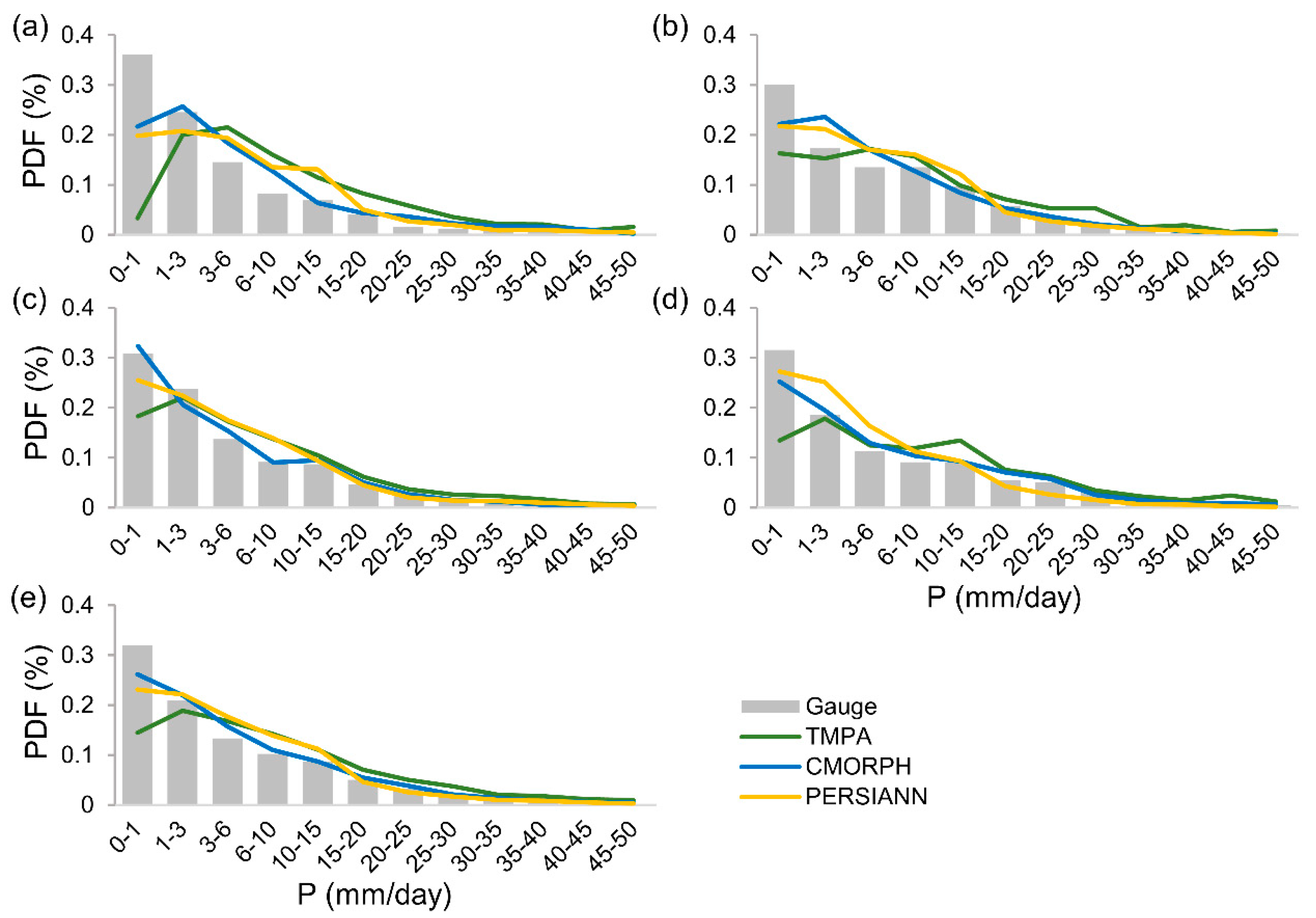
• SPPs show mixed performance skills with a seasonal dependence. Substantial differences are observed with moderate-intensity precipitation events, especially during winter, with both TMPA and PERSIANN grossly overestimating moderate-intensity precipitation. On the other hand, SPP estimates for high-intensity events are well predicted by PERSIANN but overestimated by TMPA. In the spring, all three SPPs tend to under-detect low-intensity precipitation. TMPA tends to under-detect low-intensity events and over-detect moderate- and high-intensity events; however, it is much better able to detect low-intensity events in warmer seasons.
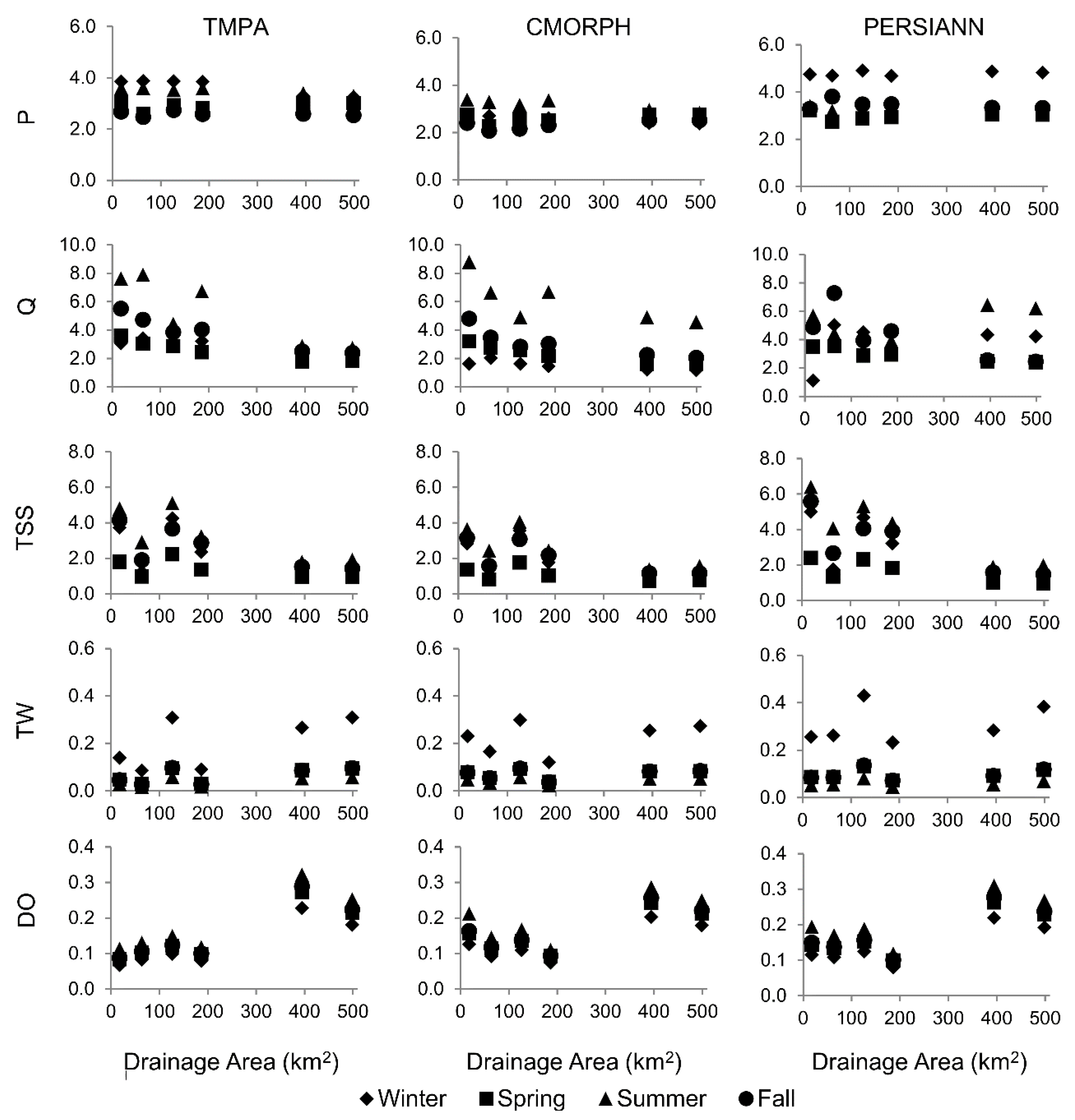
• Correlations between the SPP-simulated streamflow and reference streamflow (simulated by forcing the model with rain gauge observations) are higher with respect to the precipitation ones, although biases are also higher. Generally, random errors for the three SPPs are relatively close between streamflow and precipitation. These results indicate that the HSPF model may have a dampening effect on the streamflow error for both TMPA and CMORPH; however, due to the poor quality of the PERSIANN product, its error is actually amplified through the model, with a positive dependency on basin scale.
• For TSS, TMPA and CMORPH appear to generally outperform PERSIANN during all seasons, which is expected since similar results are noted from streamflow and simulated TSS concentrations are highly dependent on streamflow. Although the systematic error in P is amplified in TSS, the random error is not (and it is actually dampened by the model). It is worthy to mention that while larger TSS errors are generally found in summer for all three SPPs, this seasonal difference is not propagated for TSS.
• The model shows good performance when simulating TW, with TMPA and CMORPH generally outperforming PERSIANN. The error in precipitation is dampened when translated into TW and, as expected, basin scale has no influence on the precipitation-to-TW error propagation.
• Satisfactory model performance is also shown in simulated DO, with TMPA and CMORPH marginally outperforming PERSIANN. The propagation of systematic and random errors from precipitation to DO varies by season, with larger dampening effects in spring and summer for all three SPPs.

This study demonstrates that the spatiotemporal variability of SPPs, along with their different algorithms, has a quantifiable impact on water quality simulations. However, results shown here are limited by several factors. Firstly, this study was conducted using only one hydrologic model. While the HSPF model developed for the Occoquan Watershed is widely used and well calibrated and validated, other hydrologic models may propagate errors in input precipitation differently. Secondly, the model was calibrated based on rain gauge data, which may not reflect the actual distribution, extents, or magnitude of precipitation in the watershed. Thirdly, a single watershed, located in an area characterized by a temperate climate, mild topographic variation, and moderate precipitation intensity, was the focus of this study. Since it is well documented that different SPPs perform differently by climate, topography, and geographic regions, results of this study may not be directly translatable to other locations. Nonetheless, this work suggests that SPPs may be used to monitor and forecast the water quality of a hydrologic network. Future research should evaluate the applicability of SPPs for simulating water quality in other geographic and climatic regions. Additionally, future research should evaluate the effect of spatial and temporal resolution alone, by aggregating one of the fine resolution products to several coarser scales. Further, other SPPs should be investigated, such as IMERG, as well as blended and reanalysis products since these products were not considered in this study given that the use of such products would not allow for the differentiation of results between remote sensing instruments and product algorithms, which is the intent of this study: a proof of concept to access the ability of SPPs to model water quality. Furthermore, future work should investigate the use of SPPs for simulating water quality indicators during extreme hydrometeorological events (i.e., floods and droughts).

References

1. Hazra, A.; Maggioni, V.; Houser, P.; Antil, H.; Noonan, M. A Monte Carlo-based multi-objective optimization approach to merge different precipitation estimates for land surface modeling. J. Hydrol. 2019, 570, 454–462. [Google Scholar] [CrossRef]
2. Sorooshian, S.; AghaKouchak, A.; Arkin, P.; Eylander, J.; Foufoula-Georgiou, E.; Harmon, R.; Hendrickx, J.M.H.; Imam, B.; Kuligowski, R.; Skahill, B.; et al. Advanced Concepts on Remote Sensing of Precipitation at Multiple Scales. Bull. Am. Meteorol. Soc. 2011, 92, 1353–1357. [Google Scholar] [CrossRef]
3. Zeng, Q.; Chen, H.; Xu, C.-Y.; Jie, M.-X.; Chen, J.; Guo, S.-L.; Liu, J. The effect of rain gauge density and distribution on runoff simulation using a lumped hydrological modelling approach. J. Hydrol. 2018, 563, 106–122. [Google Scholar] [CrossRef]
4. Maggioni, V.; Massari, C. On the performance of satellite precipitation products in riverine flood modeling: A review. J. Hydrol. 2018, 558, 214–224. [Google Scholar] [CrossRef]
5. Sun, Q.; Miao, C.; Duan, Q.; Ashouri, H.; Sorooshian, S.; Hsu, K. A Review of Global Precipitation Data Sets: Data Sources, Estimation, and Intercomparisons. Rev. Geophys. 2018, 56, 79–107. [Google Scholar] [CrossRef] [Green Version]
6. Nijssen, B.; Lettenmaier, D.P. Effect of precipitation sampling error on simulated hydrological fluxes and states: Anticipating the Global Precipitation Measurement satellites. J. Geophys. Res. 2004, 109. [Google Scholar] [CrossRef]
7. Hong, Y.; Gochis, D.; Cheng, J.; Hsu, K.; Sorooshian, S. Evaluation of PERSIANN-CCS Rainfall Measurement Using the NAME Event Rain Gauge Network. J. Hydrometeorol. 2007, 8, 469–482. [Google Scholar] [CrossRef] [Green Version]
8. Ebert, E.E.; Janowiak, J.E.; Kidd, C. Comparison of Near-Real-Time Precipitation Estimates from Satellite Observations and Numerical Models. Bull. Am. Meteorol. Soc. 2007, 88, 47–64. [Google Scholar] [CrossRef] [Green Version]
9. Li, X.; Zhang, Q.; Xu, C.-Y. Assessing the performance of satellite-based precipitation products and its dependence on topography over Poyang Lake basin. Appl. Clim. 2014, 115, 713–729. [Google Scholar] [CrossRef]
10. Falck, A.S.; Maggioni, V.; Tomasella, J.; Vila, D.A.; Diniz, F.L.R. Propagation of satellite precipitation uncertainties through a distributed hydrologic model: A case study in the Tocantins–Araguaia basin in Brazil. J. Hydrol. 2015, 527, 943–957. [Google Scholar] [CrossRef]
11. Hossain, F.; Anagnostou, E. Assessment of current passive-microwave- and infrared-based satellite rainfall remote sensing for flood prediction. J. Geophys. Res. 2004, 109, D07102. [Google Scholar] [CrossRef] [Green Version]
12. Gebremichael, M.; Liao, G.-Y.; Yan, J. Nonparametric error model for a high resolution satellite rainfall product: NONPARAMETRIC ERROR MODEL. Water Resour. Res. 2011, 47. [Google Scholar] [CrossRef]
13. Guo, H.; Chen, S.; Bao, A.; Hu, J.; Yang, B.; Stepanian, P. Comprehensive Evaluation of High-Resolution Satellite-Based Precipitation Products over China. Atmosphere 2016, 7, 6. [Google Scholar] [CrossRef] [Green Version]
14. Hong, Y.; Hsu, K.; Moradkhani, H.; Sorooshian, S. Uncertainty quantification of satellite precipitation estimation and Monte Carlo assessment of the error propagation into hydrologic response: ERROR PROPAGATION FROM SATELLITE RAINFALL. Water Resour. Res. 2006, 42. [Google Scholar] [CrossRef] [Green Version]
15. Maggioni, V.; Vergara, H.J.; Anagnostou, E.N.; Gourley, J.J.; Hong, Y.; Stampoulis, D. Investigating the Applicability of Error Correction Ensembles of Satellite Rainfall Products in River Flow Simulations. J. Hydrometeorol. 2013, 14, 1194–1211. [Google Scholar] [CrossRef] [Green Version]
16. Mei, Y.; Nikolopoulos, E.I.; Anagnostou, E.N.; Borga, M. Evaluating Satellite Precipitation Error Propagation in Runoff Simulations of Mountainous Basins. J. Hydrometeorol. 2016, 17, 1407–1423. [Google Scholar] [CrossRef]
17. Nikolopoulos, E.I.; Anagnostou, E.N.; Hossain, F.; Gebremichael, M.; Borga, M. Understanding the Scale Relationships of Uncertainty Propagation of Satellite Rainfall through a Distributed Hydrologic Model. J. Hydrometeorol. 2010, 11, 520–532. [Google Scholar] [CrossRef]
18. Seyyedi, H.; Anagnostou, E.N.; Beighley, E.; McCollum, J. Hydrologic evaluation of satellite and reanalysis precipitation datasets over a mid-latitude basin. Atmos. Res. 2015, 164–165, 37–48. [Google Scholar] [CrossRef]
19. Yu, W.; Nakakita, E.; Kim, S.; Yamaguchi, K. Impact Assessment of Uncertainty Propagation of Ensemble NWP Rainfall to Flood Forecasting with Catchment Scale. Adv. Meteorol. 2016, 2016, 1384302. [Google Scholar] [CrossRef]
20. Wang, Z.; Zhong, R.; Lai, C.; Chen, J. Evaluation of the GPM IMERG satellite-based precipitation products and the hydrological utility. Atmos. Res. 2017, 196, 151–163. [Google Scholar] [CrossRef]
21. Zhang, J.L.; Li, Y.P.; Huang, G.H.; Wang, C.X.; Cheng, G.H. Evaluation of Uncertainties in Input Data and Parameters of a Hydrological Model Using a Bayesian Framework: A Case Study of a Snowmelt–Precipitation-Driven Watershed. J. Hydrometeorol. 2016, 17, 2333–2350. [Google Scholar] [CrossRef]
22. Elsner, M.M.; Gangopadhyay, S.; Pruitt, T.; Brekke, L.D.; Mizukami, N.; Clark, M.P. How Does the Choice of Distributed Meteorological Data Affect Hydrologic Model Calibration and Streamflow Simulations? J. Hydrometeorol. 2014, 15, 1384–1403. [Google Scholar] [CrossRef]
23. Raleigh, M.S.; Lundquist, J.D.; Clark, M.P. Exploring the impact of forcing error characteristics on physically based snow simulations within a global sensitivity analysis framework. Hydrol. Earth Syst. Sci. 2015, 19, 3153–3179. [Google Scholar] [CrossRef] [Green Version]
24. Yang, Y.; Du, J.; Cheng, L.; Xu, W. Applicability of TRMM satellite precipitation in driving hydrological model for identifying flood events: A case study in the Xiangjiang River Basin, China. Nat. Hazards 2017, 87, 1489–1505. [Google Scholar] [CrossRef]
25. Satgé, F.; Ruelland, D.; Bonnet, M.-P.; Molina, J.; Pillco, R. Consistency of satellite-based precipitation products in space and over time compared with gauge observations and snow- hydrological modelling in the Lake Titicaca region. Hydrol. Earth Syst. Sci. 2019, 23, 595–619. [Google Scholar] [CrossRef] [Green Version]
26. Riad, P.; Graefe, S.; Hussein, H.; Buerkert, A. Landscape transformation processes in two large and two small cities in Egypt and Jordan over the last five decades using remote sensing data. Landsc. Urban Plan. 2020, 197, 103766. [Google Scholar] [CrossRef]
27. Odeh, T.; Mohammad, A.H.; Hussein, H.; Ismail, M.; Almomani, T. Over-pumping of groundwater in Irbid governorate, northern Jordan: A conceptual model to analyze the effects of urbanization and agricultural activities on groundwater levels and salinity. Environ. Earth Sci. 2019, 78, 40. [Google Scholar] [CrossRef] [Green Version]
28. Guetter, A.; Georgakakos, K. Are the El Niño and La Niña Predictors of the Iowa River Seasonal Flow? J. Appl. Meteorol. 1996, 35, 690–705. [Google Scholar] [CrossRef] [Green Version]
29. Vivoni, E.R.; Entekhabi, D.; Hoffman, R.N. Error Propagation of Radar Rainfall Nowcasting Fields through a Fully Distributed Flood Forecasting Model. J. Appl. Meteor. Clim. 2007, 46, 932–940. [Google Scholar] [CrossRef]
30. Vergara, H.; Hong, Y.; Gourley, J.J.; Anagnostou, E.N.; Maggioni, V.; Stampoulis, D.; Kirstetter, P.-E. Effects of Resolution of Satellite-Based Rainfall Estimates on Hydrologic Modeling Skill at Different Scales. J. Hydrometeorol. 2014, 15, 593–613. [Google Scholar] [CrossRef] [Green Version]
31. Ehsan Bhuiyan, M.A.; Nikolopoulos, E.I.; Anagnostou, E.N.; Polcher, J.; Albergel, C.; Dutra, E.; Fink, G.; Martínez-de la Torre, A.; Munier, S. Assessment of precipitation error propagation in multi-model global water resource reanalysis. Hydrol. Earth Syst. Sci. 2019, 23, 1973–1994. [Google Scholar] [CrossRef] [Green Version]
32. Hostache, R.; Matgen, P.; Montanari, A.; Montanari, M.; Hoffmann, L.; Pfister, L. Propagation of uncertainties in coupled hydro-meteorological forecasting systems: A stochastic approach for the assessment of the total predictive uncertainty. Atmos. Res. 2011, 100, 263–274. [Google Scholar] [CrossRef]
33. Zhu, D.; Peng, D.Z.; Cluckie, I.D. Statistical analysis of error propagation from radar rainfall to hydrological models. Hydrol. Earth Syst. Sci. 2013, 17, 1445–1453. [Google Scholar] [CrossRef] [Green Version]
34. Gebregiorgis, A.S.; Hossain, F. Understanding the Dependence of Satellite Rainfall Uncertainty on Topography and Climate for Hydrologic Model Simulation. IEEE Trans. Geosci. Remote Sens. 2013, 51, 704–718. [Google Scholar] [CrossRef]
35. Neal, C.; Reynolds, B.; Rowland, P.; Norris, D.; Kirchner, J.W.; Neal, M.; Sleep, D.; Lawlor, A.; Woods, C.; Thacker, S.; et al. High-frequency water quality time series in precipitation and streamflow: From fragmentary signals to scientific challenge. Sci. Total Environ. 2012, 434, 3–12. [Google Scholar] [CrossRef] [Green Version]
36. Himanshu, S.K.; Pandey, A.; Yadav, B. Assessing the applicability of TMPA-3B42V7 precipitation dataset in wavelet-support vector machine approach for suspended sediment load prediction. J. Hydrol. 2017, 550, 103–117. [Google Scholar] [CrossRef]
37. Stryker, J.; Wemple, B.; Bomblies, A. Modeling sediment mobilization using a distributed hydrological model coupled with a bank stability model. Water Resour. Res. 2017, 53, 2051–2073. [Google Scholar] [CrossRef] [Green Version]
38. Ma, D.; Xu, Y.-P.; Gu, H.; Zhu, Q.; Sun, Z.; Xuan, W. Role of satellite and reanalysis precipitation products in streamflow and sediment modeling over a typical alpine and gorge region in Southwest China. Sci. Total Environ. 2019, 685, 934–950. [Google Scholar] [CrossRef]
39. Bezak, N.; Rusjan, S.; Fijavž, M.K.; Mikoš, M.; Šraj, M. Estimation of Suspended Sediment Loads Using Copula Functions. Water 2017, 9, 628. [Google Scholar] [CrossRef] [Green Version]
40. Chang, C.-H.; Cai, L.-Y.; Lin, T.-F.; Chung, C.-L.; van der Linden, L.; Burch, M. Assessment of the Impacts of Climate Change on the Water Quality of a Small Deep Reservoir in a Humid-Subtropical Climatic Region. Water 2015, 7, 1687–1711. [Google Scholar] [CrossRef] [Green Version]
41. Gelca, R.; Hayhoe, K.; Scott-Fleming, I.; Crow, C.; Dawson, D.; Patiño, R. Climate-water quality relationships in Texas reservoirs: Climate-Water Quality Relationships in Texas Reservoirs. Hydrol. Process. 2016, 30, 12–29. [Google Scholar] [CrossRef]
42. Hayashi, S.; Murakami, S.; Watanabe, M.; Bao-Hua, X. HSPF Simulation of Runoff and Sediment Loads in the Upper Changjiang River Basin, China. J. Environ. Eng. 2004, 130, 801–815. [Google Scholar] [CrossRef]
43. Jeznach, L.C.; Hagemann, M.; Park, M.-H.; Tobiason, J.E. Proactive modeling of water quality impacts of extreme precipitation events in a drinking water reservoir. J. Environ. Manag. 2017, 201, 241–251. [Google Scholar] [CrossRef] [PubMed]
44. Johnson, T.E.; Butcher, J.B.; Parker, A.; Weaver, C.P. Investigating the Sensitivity of U.S. Streamflow and Water Quality to Climate Change: U.S. EPA Global Change Research Program’s 20 Watersheds Project. J. Water Resour. Plan. Manag. 2012, 138, 453–464. [Google Scholar] [CrossRef]
45. Murdoch, P.S.; Baron, J.S.; Miller, T.L. Potential Effects of Climate Change on Surface-Water Quality in North America. J. Am. Water Resour. Assoc. 2000, 36, 347–366. [Google Scholar] [CrossRef]
46. Soler, M.; Regüés, D.; Latron, J.; Gallart, F. Frequency–magnitude relationships for precipitation, stream flow and sediment load events in a small Mediterranean basin (Vallcebre basin, Eastern Pyrenees). Catena 2007, 71, 164–171. [Google Scholar] [CrossRef]
47. Thorne, O.; Fenner, R.A. The impact of climate change on reservoir water quality and water treatment plant operations: A UK case study: The impact of climate change on reservoir water quality and WTP operations. Water Environ. J. 2011, 25, 74–87. [Google Scholar] [CrossRef]
48. Solakian, J.; Maggioni, V.; Lodhi, A.; Godrej, A. Investigating the use of satellite-based precipitation products for monitoring water quality in the Occoquan Watershed. J. Hydrol. Reg. Stud. 2019, 26, 100630. [Google Scholar] [CrossRef]
49. U.S. Environmental Protection Agency, Region 3, Water Protection Division. Chesapeake Bay Total Maximum Daily Load for Nitrogen, Phosphorus and Sediment. 2010. Available online: https://www.epa.gov/chesapeake-bay-tmdl/chesapeake-bay-tmdl-document (accessed on 1 November 2020).
50. Huffman, G.J.; Bolvin, D.T.; Nelkin, E.J. The TRMM Multi-Satellite Precipitation Analysis (TMPA). In Satellite Rainfall Applications for Surface Hydrology; Gebremichael, M., Hossain, F., Eds.; Springer: Dordrecht, The Netherlands, 2010; pp. 3–22. [Google Scholar] [CrossRef] [Green Version]
51. Joyce, R.J.; Janowiak, J.E.; Arkin, P.A.; Xie, P. CMORPH: A Method that Produces Global Precipitation Estimates from Passive Microwave and Infrared Data at High Spatial and Temporal Resolution. J. Hydrometeorol. 2004, 5, 487–503. [Google Scholar] [CrossRef]
52. Hsu, K.; Behrangi, A.; Imam, B.; Sorooshian, S. Extreme Precipitation Estimation Using Satellite-Based PERSIANN-CCS Algorithm. In Satellite Rainfall Applications for Surface Hydrology; Gebremichael, M., Hossain, F., Eds.; Springer: Dordrecht, The Netherlands, 2010. [Google Scholar] [CrossRef]
53. Huffman, G.J.; Bolvin, D.T.; Nelkin, E.J.; Wolff, D.B.; Adler, R.F.; Gu, G.; Hong, Y.; Bowman, K.P.; Stocker, E.F. The TRMM Multisatellite Precipitation Analysis (TMPA): Quasi-Global, Multiyear, Combined-Sensor Precipitation Estimates at Fine Scales. J. Hydrometeorol. 2007, 8, 38–55. [Google Scholar] [CrossRef]
54. Tropical Rainfall Measuring Mission (TRMM). TRMM (TMPA) Rainfall Estimate L3 3 Hour 0.25 Degree × 0.25 Degree V7, Greenbelt, MD, Goddard Earth Sciences Data and Information Services Center (GES DISC). 2011. Available online: https://pmm.nasa.gov/data-access/downloads/TRMM (accessed on 22 May 2018). [CrossRef]
55. Xie, P.; Joyce, R.; Wu, S.; Yoo, S.-H.; Yarosh, Y.; Sun, F.; Lin, R. Reprocessed, Bias-Corrected CMORPH Global High-Resolution Precipitation Estimates from 1998. J. Hydrometeorol. 2017, 18, 1617–1641. [Google Scholar] [CrossRef]
56. Xie, P.; Joyce, R.; Wu, S.; Yoo, S.-H.; Yarosh, Y.; Sun, F.; Lin, R. NOAA CDR Program (2019): NOAA Climate Data Record (CDR) of CPC Morphing Technique (CMORPH) High Resolution Global Precipitation Estimates, Version 1 [8 km × 8 km, 30 min]. NOAA National Centers for Environmental Information. Available online: ftp://ftp.cpc.ncep.noaa.gov/precip/global_CMORPH/30min_8km (accessed on 24 May 2018).
57. Hsu, K.; Gao, X.; Sorooshian, S.; Gupta, H.V. Precipitation Estimation from Remotely Sensed Information Using Artificial Neural Networks. J. Appl. Meteorol. 1997, 36, 1176–1190. [Google Scholar] [CrossRef]
58. Center for Hydrometeorology and Remote Sensing, PERSIANN-CCS [0.04 × 0.04 degree, 30 min]. Available online: http://chrsdata.eng.uci.edu/ (accessed on 23 April 2018).
59. Sorooshian, S.; Hsu, K.; Gao, X.; Gupta, H.V.; Imam, B.; Braithwaite, D. Evaluation of PERSIANN System Satellite-Based Estimates of Tropical Rainfall. Bull. Am. Meteorogogical Soc. 2000, 81, 2035–2046. [Google Scholar] [CrossRef] [Green Version]
60. Albek, M.; Bakır Öğütveren, Ü.; Albek, E. Hydrological modeling of Seydi Suyu watershed (Turkey) with HSPF. J. Hydrol. 2004, 285, 260–271. [Google Scholar] [CrossRef]
61. Duda, P.; Hummel, P.; Donigian, A.S., Jr.; Imhoff, A.C. BASINS/HSPF: Model Use, Calibration, and Validation. Trans. Asabe 2012, 55, 1523–1547. [Google Scholar] [CrossRef]
62. Li, Z.; Liu, H.; Luo, C.; Li, Y.; Li, H.; Pan, J.; Jiang, X.; Zhou, Q.; Xiong, Z. Simulation of runoff and nutrient export from a typical small watershed in China using the Hydrological Simulation Program–Fortran. Environ. Sci. Pollut. Res. 2015, 22, 7954–7966. [Google Scholar] [CrossRef]
63. Mishra, A.; Kar, S.; Singh, V.P. Determination of runoff and sediment yield from a small watershed in sub-humid subtropics using the HSPF model. Hydrol. Process. 2007, 21, 3035–3045. [Google Scholar] [CrossRef]
64. Huo, S.-C.; Lo, S.-L.; Chiu, C.-H.; Chiueh, P.-T.; Yang, C.-S. Assessing a fuzzy model and HSPF to supplement rainfall data for nonpoint source water quality in the Feitsui reservoir watershed. Environ. Model. Softw. 2015, 72, 110–116. [Google Scholar] [CrossRef]
65. Stern, M.; Flint, L.; Minear, J.; Flint, A.; Wright, S. Characterizing Changes in Streamflow and Sediment Supply in the Sacramento River Basin, California, Using Hydrological Simulation Program—FORTRAN (HSPF). Water 2016, 8, 432. [Google Scholar] [CrossRef] [Green Version]
66. Diaz-Ramirez, J.; Johnson, B.; McAnally, W.; Martin, J.; Camacho, R. Estimation and Propagation of Parameter Uncertainty in Lumped Hydrological Models: A Case Study of HSPF Model Applied to Luxapallila Creek Watershed in Southeast USA. J. Hydrogeol. Hydrol. Eng. 2013, 2. [Google Scholar] [CrossRef]
67. Wu, J.; Yu, S.L.; Zou, R. A Water quality-based approach for watershed wide bmp strategies. JAWRA J. Am. Water Resour. Assoc. 2006, 42, 1193–1204. [Google Scholar] [CrossRef]
68. Young, C.B.; Bradley, A.A.; Krajewski, W.F.; Kruger, A.; Morrissey, M.L. Evaluating NEXRAD Multisensor Precipitation Estimates for Operational Hydrologic Forecasting. J. Hydrometeorol. 2000, 1, 14. [Google Scholar] [CrossRef] [Green Version]
69. Xu, Z.; Godrej, A.N.; Grizzard, T.J. The hydrological calibration and validation of a complexly-linked watershed–reservoir model for the Occoquan watershed, Virginia. J. Hydrol. 2007, 345, 167–183. [Google Scholar] [CrossRef]
70. Schaefer, J.T. The Critical Success Index as an Indicator of Warning Skill. Weather Forecast. 1990, 570–575. [Google Scholar] [CrossRef] [Green Version]
71. Roebber, P.J. Visualizing Multiple Measures of Forecast Quality. Weather Forecast. 2009, 24, 601–608. [Google Scholar] [CrossRef] [Green Version]
72. Taylor, K.E. Summarizing multiple aspects of model performance in a single diagram. J. Geophys. Res. Atmos. 2001, 106, 7183–7192. [Google Scholar] [CrossRef]
73. Cox, B.A.; Whitehead, P.G. Impacts of climate change scenarios on dissolved oxygen in the River Thames, UK. Hydrol. Res. 2009, 40, 138–152. [Google Scholar] [CrossRef]
74. Irby, I.D.; Friedrichs, M.A.M.; Da, F.; Hinson, K.E. The competing impacts of climate change and nutrient reductions on dissolved oxygen in Chesapeake Bay. Biogeosciences 2018, 15, 2649–2668. [Google Scholar] [CrossRef] [Green Version]
75. Moreno-Rodenas, A.M.; Tscheikner-Gratl, F.; Langeveld, J.G.; Clemens, F.H.L.R. Uncertainty analysis in a large-scale water quality integrated catchment modelling study. Water Res. 2019, 158, 46–60. [Google Scholar] [CrossRef]
Figure 1. Study area showing the Occoquan Watershed boundary, 7 catchments, 87 segments, topography, major streams, major waterbodies, locations of stream monitoring stations, and the locations of model evaluation points (S47, S86, and S79 coincide with stream monitoring stations).
Remotesensing 12 03728 g001
Figure 2. Cumulative 5-year areal-weighted and segment-aggregated (AWSA) precipitation for each segment in the Occoquan Watershed for the (a) rain gauge network and satellite-based precipitation products (SPPs): (b) TMPA, (c) CMORPH, and (d) PERSIANN including the spatial resolution of SPP pixels at 0.25°, 0.07°, and 0.04°, respectively.
Remotesensing 12 03728 g002
Figure 3. Probability density functions of daily AWSA precipitation measured across the watershed (87 segments) from rain gauge observations (gray histograms) and SPP estimates (colored lines) during (a) winter, (b) spring, (c) summer, (d) fall, and (e) 5-year period.
Remotesensing 12 03728 g003
Figure 4. Seasonal (a) performance diagram and (b) Taylor diagram of AWSA daily precipitation between gauge-based observation and SPPs over the 5-year study period.
Remotesensing 12 03728 g004
Figure 5. Logarithmic density scatter plots between the gauge-based reference and SPP-simulated model output for TMPA, CMORPH, and PERSIANN during the 5-year study period for P, Q, TSS, TW, and DO.
Remotesensing 12 03728 g005
Figure 6. Seasonal analysis of absolute bias at each model evaluation point as a function of basin scale (km2) for P, Q, TSS, TW, and DO between gauge-based records and SPPs TMPA, CMORPH, and PERSIANN during the 5-year study period.
Remotesensing 12 03728 g006
Figure 7. Seasonal analysis of rRMSE at each model evaluation point as a function of basin scale (km2) for P, Q, TSS, TW, and DO between gauge-based records and SPPs TMPA, CMORPH, and PERSIANN during the 5-year study period.
Remotesensing 12 03728 g007
Figure 8. Seasonal analysis of bias (B) error propagation at each model evaluation point as a function of basin scale (km2) for Q, TW, TSS, and DO between gauge-based records and SPPs TMPA, CMORPH, and PERSIANN during the 5-year study period.
Remotesensing 12 03728 g008
Figure 9. Seasonal analysis of rRMSE error propagation at each model evaluation point as a function of basin scale (km2) for Q, TW, TSS, and DO between gauge-based records and SPPs TMPA, CMORPH, and PERSIANN during the 5-year study period.
Remotesensing 12 03728 g009