DInSAR for Road Infrastructure Monitoring: Case Study Highway Network of Rome Metropolitan (Italy)

 ,
,  and
and 
Abstract
1. Introduction
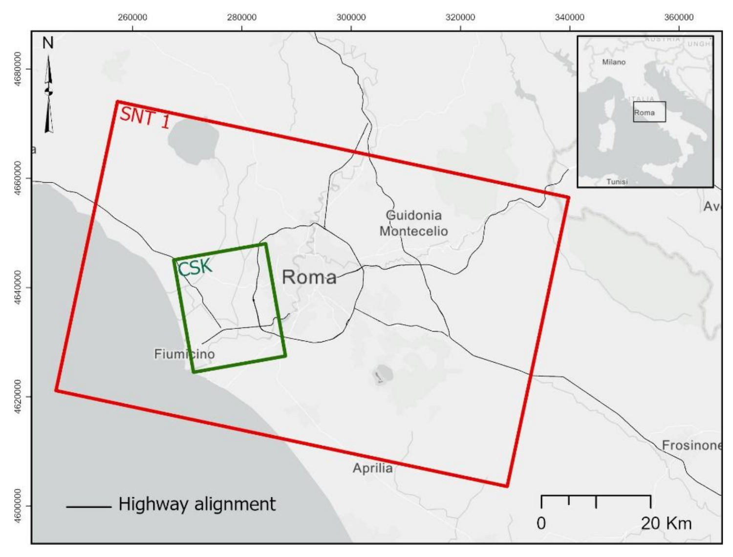
1.1. Study Area
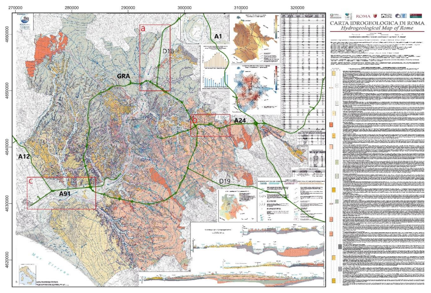
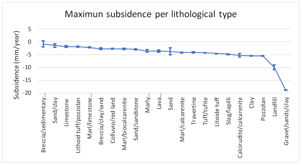
1.2. Geological Setting
2. Materials and Methods
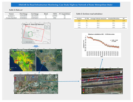
2.1. Dataset
2.2. Interferometric Processing
2.2.1. SNAP-StaMPS PSI
2.2.2. SBAS Technique
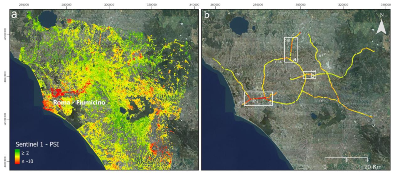
3. Results 1: Sentinel-1 Data
3.1. Low Resolution Analysis: Highway Network of Rome Metropolitan
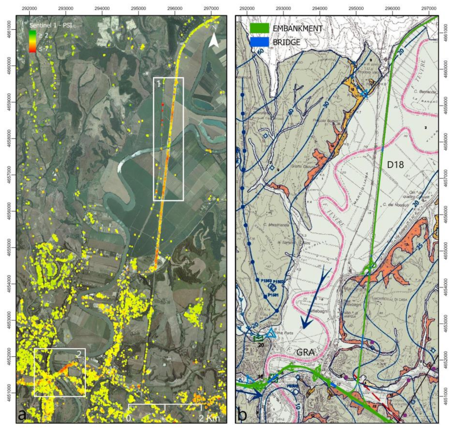
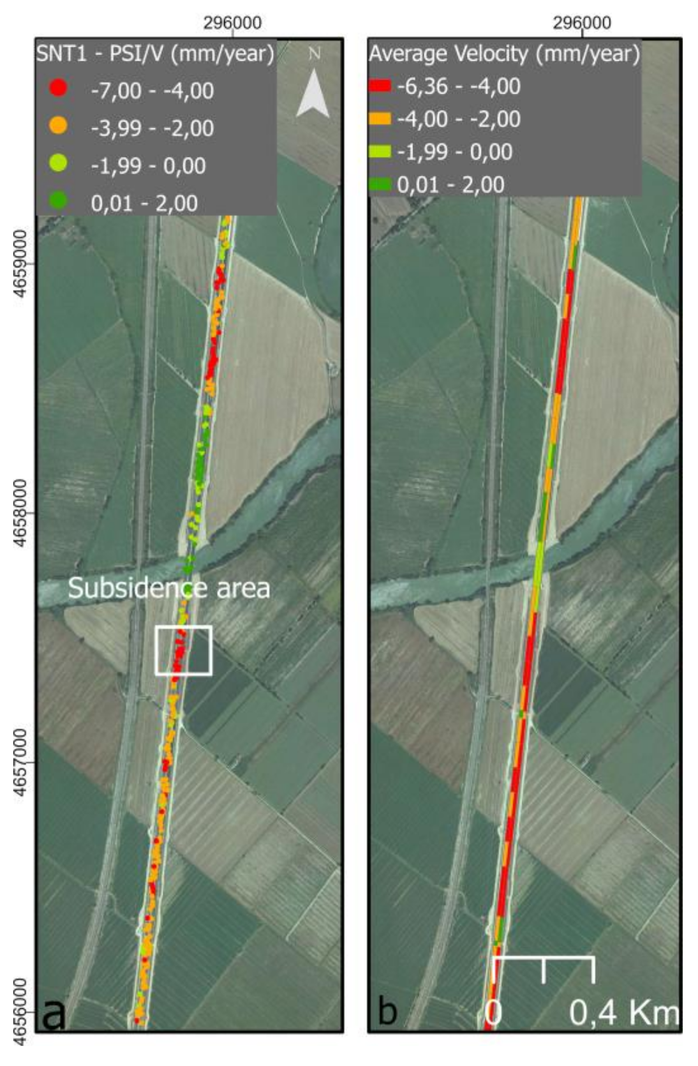
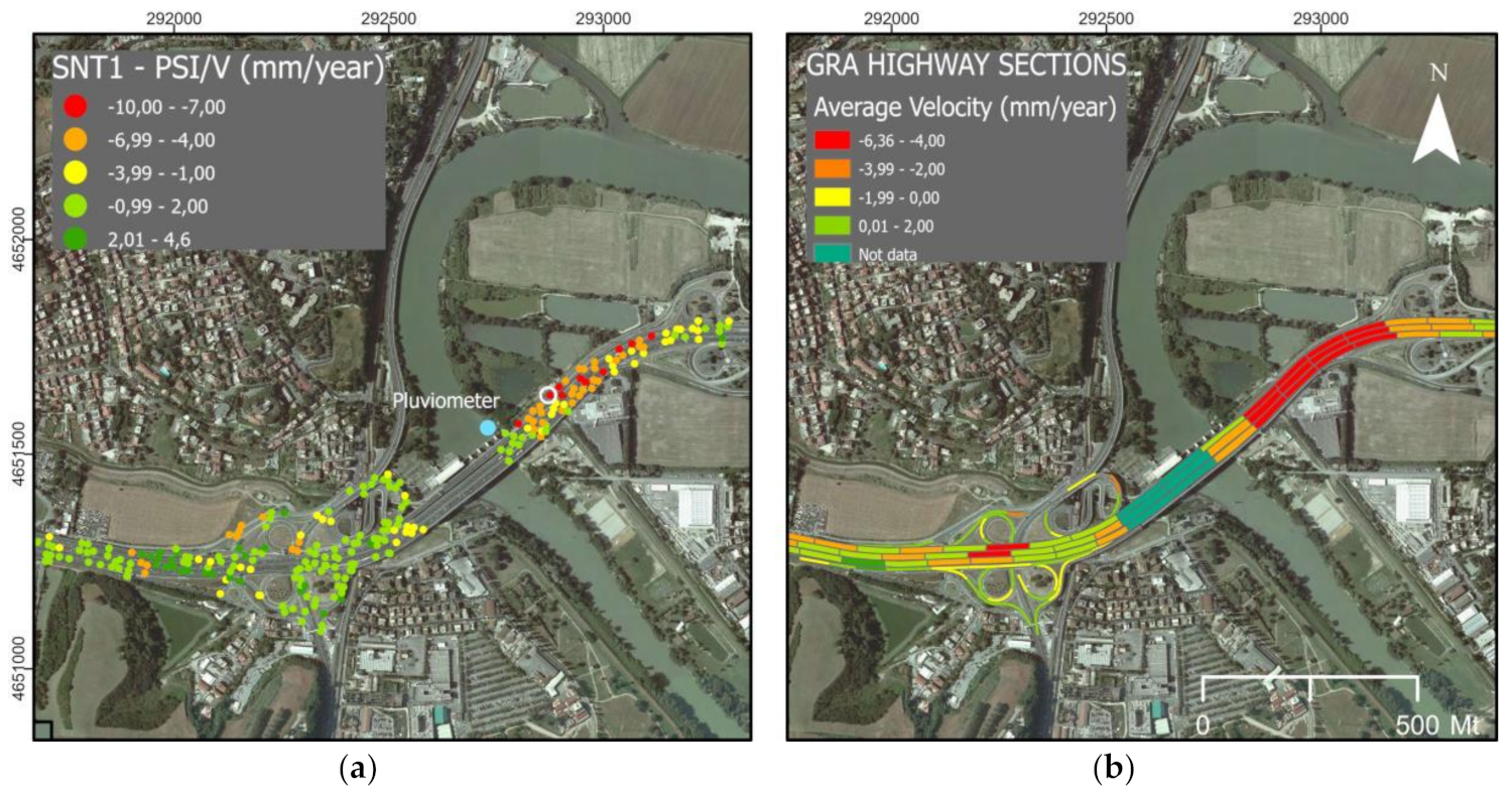
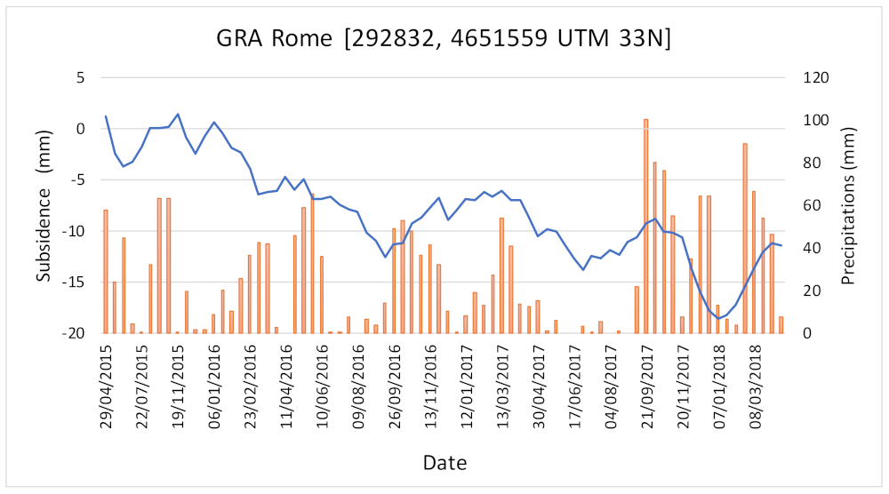
3.1.1. Area (a): D18–GRA Highways
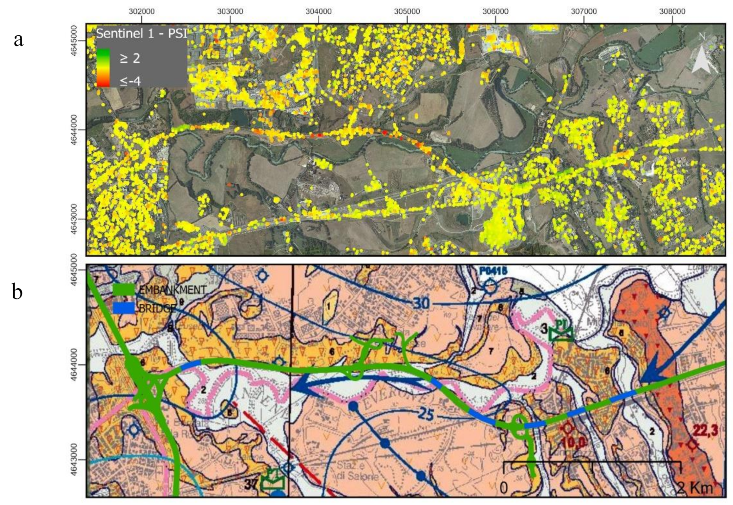
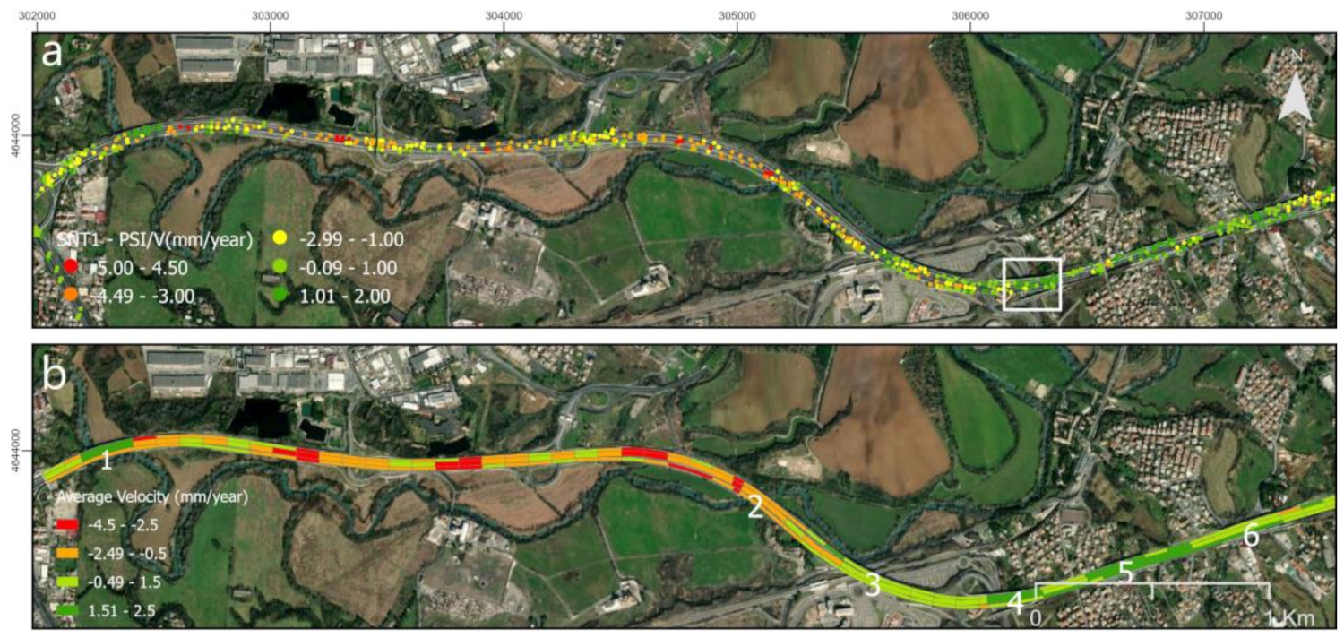
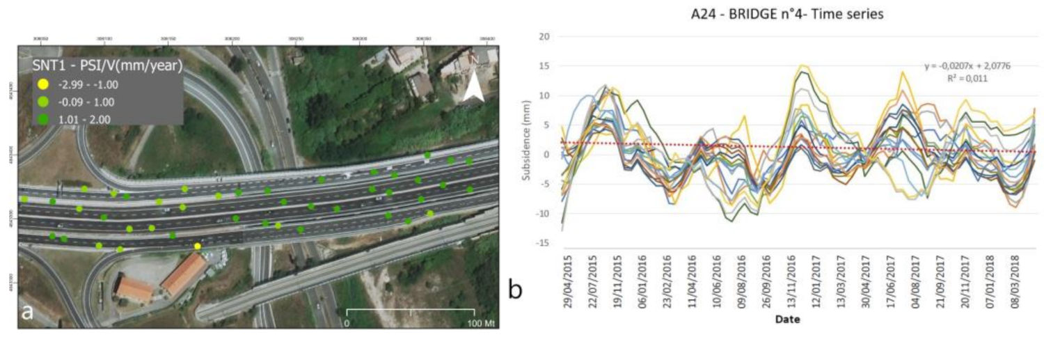
3.1.2. Area (b): A24 Highway
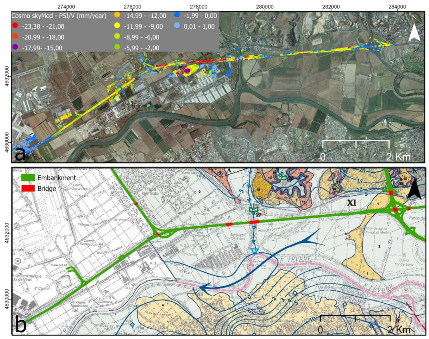
4. Results 2: Cosmo-SkyMed Data
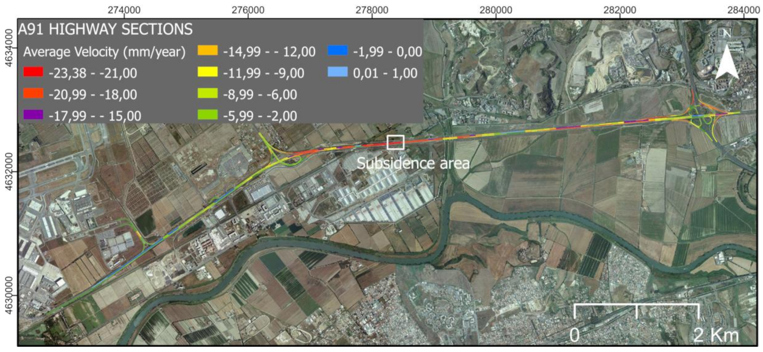
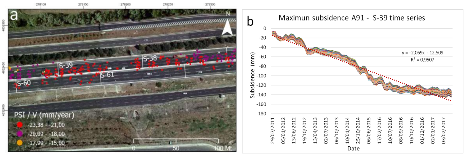
4.1. High Resolution Analysis: A91 Highway
A91 Highway (Rome-Fiumicino)
- S-39 and S-38, for the carriageway in the direction of Fiumicino; and
- S-60 and S-61 for the carriageway to Rome.
5. Conclusions
Author Contributions
Funding
Acknowledgments
Conflicts of Interest
References
- Arangio, S.; Bontempi, F.; Ciampoli, M. Structural integrity monitoring for dependability. Struct. Infrastruct. Eng. 2011, 7, 75–86. [Google Scholar] [CrossRef]
- Chang, L.; Dollevoet, R.P.B.J.; Hanssen, R.F. Monitoring Line-Infrastructure with Multisensor SAR Interferometry: Products and Performance Assessment Metrics. IEEE J. Sel. Top. Appl. Earth Obs. Remote Sens. 2018, 11, 1593–1605. [Google Scholar] [CrossRef]
- Ferretti, A.; Fumagalli, A.; Novali, F.; Prati, C.; Rocca, F.; Rucci, A. A New Algorithm for Processing Interferometric Data-Stacks: SqueeSAR. IEEE Trans. Geosci. Remote Sens. 2011, 49, 3460–3470. [Google Scholar] [CrossRef]
- Ferretti, A.; Prati, C.; Rocca, F. Nonlinear subsidence rate estimation using permanent scatterers in differential SAR interferometry. IEEE Trans. Geosci. Remote Sens. 2000, 38, 2202–2212. [Google Scholar] [CrossRef]
- Lanari, R.; Mora, O.; Manunta, M.; Mallorqui, J.J.; Berardino, P.; Sansosti, E. A small-baseline approach for investigating deformations on full-resolution differential SAR interferograms. IEEE Trans. Geosci. Remote Sens. 2004, 42, 1377–1386. [Google Scholar] [CrossRef]
- Werner, C.; Wegmuller, U.; Strozzi, T.; Wiesmann, A. Interferometric point target analysis for deformation mapping. In Proceedings of the International Geoscience and Remote Sensing Symposium (IGARSS), Toulouse, France, 21–25 July 2003; Volume 7, pp. 4362–4364. [Google Scholar]
- Bonano, M.; Manunta, M.; Pepe, A.; Paglia, L.; Lanari, R. From Previous C-Band to New X-Band SAR Systems: Assessment of the DInSAR Mapping Improvement for Deformation Time-Series Retrieval in Urban Areas. IEEE Trans. Geosci. Remote Sens. 2013, 51, 1973–1984. [Google Scholar] [CrossRef]
- Casu, F.; Manzo, M.; Lanari, R. A quantitative assessment of the SBAS algorithm performance for surface deformation retrieval from DInSAR data. Remote Sens. Environ. 2006, 102, 195–210. [Google Scholar] [CrossRef]
- Crosetto, M.; Monserrat, O.; Cuevas, M.; Crippa, B. Spaceborne Differential SAR Interferometry: Data Analysis Tools for Deformation Measurement. Remote Sens. 2011, 3, 305–318. [Google Scholar] [CrossRef]
- Papageorgiou, E.; Foumelis, M.; Trasatti, E.; Ventura, G.; Raucoules, D.; Mouratidis, A. Multi-Sensor SAR Geodetic Imaging and Modelling of Santorini Volcano Post-Unrest Response. Remote Sens. 2019, 11, 259. [Google Scholar] [CrossRef]
- Aslan, G.; Foumelis, M.; Raucoules, D.; De Michele, M.; Bernardie, S.; Çakir, Z. Landslide Mapping and Monitoring Using Persistent Scatterer Interferometry (PSI) Technique in the French Alps. Remote Sens. 2020, 12, 1305. [Google Scholar] [CrossRef]
- Lemoine, A.; Briole, P.; Bertil, D.; Roullé, A.; Foumelis, M.; Thinon, I.; Raucoules, D.; De Michele, M.; Valty, P.; Colomer, R.H. The 2018–2019 seismo-volcanic crisis east of Mayotte, Comoros islands: Seismicity and ground deformation markers of an exceptional submarine eruption. Geophys. J. Int. 2020, 223, 22–44. [Google Scholar] [CrossRef]
- Foumelis, M.; Papageorgiou, E.; Stamatopoulos, C. Episodic ground deformation signals in Thessaly Plain (Greece) revealed by data mining of SAR interferometry time series. Int. J. Remote Sens. 2016, 37, 3696–3711. [Google Scholar] [CrossRef]
- Bovenga, F.; Nitti, D.O.; Fornaro, G.; Radicioni, F.; Stoppini, A.; Brigante, R. Using C/X-band SAR interferometry and GNSS measurements for the Assisi landslide analysis. Int. J. Remote Sens. 2013, 34, 4083–4104. [Google Scholar] [CrossRef]
- Chen, F.; Wu, Y.; Zhang, Y.; Parcharidis, I.; Ma, P.; Xiao, R.; Xu, J.; Zhou, W.; Tang, P.; Foumelis, M. Surface Motion and Structural Instability Monitoring of Ming Dynasty City Walls by Two-Step Tomo-PSInSAR Approach in Nanjing City, China. Remote Sens. 2017, 9, 371. [Google Scholar] [CrossRef]
- Parcharidis, I.; Foumelis, M.; Benekos, G.; Kourkouli, P.; Stamatopoulos, C.A.; Stramondo, S. Time series synthetic aperture radar interferometry over the multispan cable-stayed Rio-Antirio Bridge (central Greece): Achievements and constraints. J. Appl. Remote Sens. 2015, 9, 96082. [Google Scholar] [CrossRef]
- D’Aranno, P.; Di Benedetto, A.; Fiani, M.; Marsella, M. Remote Sensing Technologies for Linear Infrastructure Monitoring. ISPRS Int. Arch. Photogramm. Remote Sens. Spat. Inf. Sci. 2019, 2, 461–468. [Google Scholar] [CrossRef]
- Milillo, P.; Giardina, G.; Perissin, D.; Milillo, G.; Coletta, A.; Terranova, C. Pre-Collapse Space Geodetic Observations of Critical Infrastructure: The Morandi Bridge, Genoa, Italy. Remote Sens. 2019, 11, 1403. [Google Scholar] [CrossRef]
- Sousa, J.J.; Bastos, L.F.S. Multi-temporal SAR interferometry reveals acceleration of bridge sinking before collapse. Nat. Hazards Earth Syst. Sci. 2013, 13, 659–667. [Google Scholar] [CrossRef]
- Lazecky, M.; Hlaváčová, I.; Bakon, M.; Sousa, J.J.; Perissin, D.; Patricio, G. Bridge Displacements Monitoring Using Space-Borne X-Band SAR Interferometry. IEEE J. Sel. Top. Appl. Earth Obs. Remote Sens. 2016, 10, 205–210. [Google Scholar] [CrossRef]
- Hu, F.; Van Leijen, F.; Chang, L.; Wu, J.; Hanssen, R.F. Monitoring Deformation along Railway Systems Combining Multi-Temporal InSAR and LiDAR Data. Remote Sens. 2019, 11, 2298. [Google Scholar] [CrossRef]
- Luo, Q.; Zhou, G.; Perissin, D. Monitoring of Subsidence along Jingjin Inter-City Railway with High-Resolution TerraSAR-X MT-InSAR Analysis. Remote Sens. 2017, 9, 717. [Google Scholar] [CrossRef]
- Chang, L.; Dollevoet, R.P.B.J.; Hanssen, R.F. Nationwide Railway Monitoring Using Satellite SAR Interferometry. IEEE J. Sel. Top. Appl. Earth Obs. Remote Sens. 2016, 10, 596–604. [Google Scholar] [CrossRef]
- Perissin, D.; Wang, Z.; Lin, H. Shanghai subway tunnels and highways monitoring through Cosmo-SkyMed Persistent Scatterers. ISPRS J. Photogramm. Remote Sens. 2012, 73, 58–67. [Google Scholar] [CrossRef]
- Martí, J.G.; Nevard, S.; Sanchez, J. The Use of InSAR (Interferometric Synthetic Aperture Radar) to Complement Control of Construction and Protect Third Party Assets; Crossrail Learning Legacy Report; Crossrail Ltd.: London, UK, 2017. [Google Scholar]
- Milillo, P.; Giardina, G.; DeJong, M.J.; Perissin, D.; Milillo, G. Multi-Temporal InSAR Structural Damage Assessment: The London Crossrail Case Study. Remote Sens. 2018, 10, 287. [Google Scholar] [CrossRef]
- Vaccari, A.; Batabyal, T.; Tabassum, N.; Hoppe, E.; Bruckno, B.S.; Acton, S.T. Integrating Remote Sensing Data in Decision Support Systems for Transportation Asset Management. Transp. Res. Rec. J. Transp. Res. Board 2018, 2672, 23–35. [Google Scholar] [CrossRef]
- Infante, D.; Di Martire, D.; Confuorto, P.; Tessitore, S.; Ramondini, M.; Calcaterra, D. Differential Sar Interferometry Technique for Control of Linear Infrastructures Affected by Ground Instability Phenomena. ISPRS Int. Arch. Photogramm. Remote Sens. Spat. Inf. Sci. 2018, 3, 251–258. [Google Scholar] [CrossRef]
- Foumelis, M.; Blasco, J.M.D.; Desnos, Y.-L.; Engdahl, M.; Fernandez, D.; Veci, L.; Lu, J.; Wong, C. ESA SNAP-StaMPS Integrated Processing for Sentinel-1 Persistent Scatterer Interferometry. In Proceedings of the 2018 IEEE International Geoscience and Remote Sensing Symposium, Valencia, Spain, 22–27 July 2018; pp. 1364–1367. [Google Scholar] [CrossRef]
- Berardino, P.; Fornaro, G.; Lanari, R.; Sansosti, E. A new algorithm for surface deformation monitoring based on small baseline differential SAR interferograms. IEEE Trans. Geosci. Remote Sens. 2002, 40, 2375–2383. [Google Scholar] [CrossRef]
- Funiciello, R.; Heiken, G.; De Rita, D. I Sette Colli: Guida Geologica a Una Roma Mai Vista; Raffaello Cortina Editore: Milano, Italy, 2006. [Google Scholar]
- Bellotti, P.; Chiocci, F.L.; Milli, S.; Tortora, P.; Valeri, P. Sequence Stratigraphy and Depositional Setting of the Tiber Delta: Integration of High-resolution Seismics, Well Logs, and Archeological Data. J. Sediment. Res. 1994, 64, 416–432. [Google Scholar] [CrossRef]
- Chiocci, F.L.; Milli, S. Construction of a chronostratigraphic diagram for a high frequency sequence: The 20 ky B.P. to present Tiber depositional sequence. Il Quat. 1995, 8, 339–348. [Google Scholar]
- Milli, S. Depositional setting and high-frequency sequence stratigraphy of the middle-upper Pleistocene to Holocene deposits of the Roman basin. Geol. Romana. 1997, 33, 99–136. [Google Scholar]
- Giraudi, C. Evoluzione tardo-olocenica del delta del Tevere. Il Quat. 2004, 17, 477–492. [Google Scholar]
- Bellotti, P.; Calderoni, G.; Di Rita, F.; D’Orefice, M.; D’Amico, C.; Esu, D.; Magri, D.; Martinez, M.P.; Tortora, P.; Valeri, P. The Tiber river delta plain (central Italy): Coastal evolution and implications for the ancient Ostia Roman settlement. Holocene 2011, 21, 1105–1116. [Google Scholar] [CrossRef]
- Milli, S.; D’Ambrogi, C.; Bellotti, P.; Calderoni, G.; Carboni, M.G.; Celant, A.; Di Bella, L.; Di Rita, F.; Frezza, V.; Magri, D.; et al. The transition from wave-dominated estuary to wave-dominated delta: The Late Quaternary stratigraphic architecture of Tiber River deltaic succession (Italy). Sediment. Geol. 2013, 284, 159–180. [Google Scholar] [CrossRef]
- Milli, S.; Mancini, M.; Moscatelli, M.; Stigliano, F.; Marini, M.; Cavinato, G.P. From river to shelf, anatomy of a high-frequency depositional sequence: The Late Pleistocene to Holocene Tiber depositional sequence. Sedimentol. 2016, 63, 1886–1928. [Google Scholar] [CrossRef]
- La Vigna, F.; Mazza, R.; Amanti, M.; Di Salvo, C. Hydrogeological Map of Rome; Roma Capitale: Rome, Italy, 2015. [Google Scholar]
- Bozzano, F.; Esposito, C.; Mazzanti, P.; Patti, M.; Scancella, S. Imaging Multi-Age Construction Settlement Behaviour by Advanced SAR Interferometry. Remote Sens. 2018, 10, 1137. [Google Scholar] [CrossRef]
- Cappelli, G.; Mazza, R.; Taviani, S. Acque sotterranee nella città di Roma. Mem. Descr. Carta Geol. d’It. 2008, 80, 221–245. [Google Scholar]
- Capelli, G.; Mastrorillo, L.; Mazza, R.; Petitta, M.; Baldoni, T.; Banzato, F.; Cascone, D.; Di Salvo, C.; La Vigna, F.; Taviani, S.; et al. Carta Idrogeologica del Territorio della Regione Lazio, Scala 1:100.000; S.EL.CA.: Firenze, Italy, 2012. [Google Scholar]
- Blasco, J.M.D.; Foumelis, M.; Stewart, C.; Hooper, A. Measuring Urban Subsidence in the Rome Metropolitan Area (Italy) with Sentinel-1 SNAP-StaMPS Persistent Scatterer Interferometry. Remote Sens. 2019, 11, 129. [Google Scholar] [CrossRef]
- ESA Sentinel-Topsar Processing. Available online: https://sentinel.esa.int/web/sentinel/technical-guides/sentinel-1-sar/products-algorithms/level-1-algorithms/topsar-processing (accessed on 25 July 2020).
- Tapete, D.; Cigna, F. COSMO-SkyMed SAR for Detection and Monitoring of Archaeological and Cultural Heritage Sites. Remote Sens. 2019, 11, 1326. [Google Scholar] [CrossRef]
- Blasco Jose Manuel and Foumelis Michael, GitHub/SNAPtoStsMPS Toolbox: Delgado. Available online: https://github.com/mdelgadoblasco/snap2stamps/ (accessed on 25 July 2020).
- Open Data: Copernicus Open Access HUB. Available online: https://scihub.copernicus.eu/ (accessed on 18 July 2020).
- Supplementary Materials: Sentinel-1 PS LOS Displacement Rates over the Period April 2015–May 2018 in WGS84 Projection Are Provided in Environmental Systems Research Institute (ESRI) Shapefile Format for Both Ascending and Descending Datasets. Available online: www.mdpi.com/2072-4292/11/2/129/s1 (accessed on 31 July 2020).
- Blasco, J.M.D. Michael Foumelis: Automated SNAP Sentinel-1 DInSAR Processing for StaMPS PSI with Open Source Tools. 2018. Available online: https://zenodo.org/record/1322353#.XxqafUUzY2w (accessed on 31 July 2020).
- Hooper, A.; Bekaert, D.; Spaans, K.; Arıkan, M. Recent advances in SAR interferometry time series analysis for measuring crustal deformation. Tectonophysics 2012, 514–517, 1–13. [Google Scholar] [CrossRef]
- Hooper, A.; Zebker, H.; Segall, P.; Kampes, B. A New Method for Measuring Deformation on Volcanoes and Other Natural Terrains Using InSAR Persistent Scatterers. Geophys. Res. Lett. 2004, 31. [Google Scholar] [CrossRef]
- Scifoni, S.; Bonano, M.; Marsella, M.; Sonnessa, A.; Tagliafierro, V.; Manunta, M.; Lanari, R.; Ojha, C.; Sciotti, M. On the joint exploitation of long-term DInSAR time series and geological information for the investigation of ground settlements in the town of Roma (Italy). Remote Sens. Environ. 2016, 182, 113–127. [Google Scholar] [CrossRef]
- Bonano, M.; Manunta, M.; Marsella, M.; Lanari, R. Long-term ERS/ENVISAT deformation time-series generation at full spatial resolution via the extended SBAS technique. Int. J. Remote Sens. 2012, 33, 4756–4783. [Google Scholar] [CrossRef]
- Zeni, G.; Bonano, M.; Casu, F.; Manunta, M.; Manzo, M.; Marsella, M.; Pepe, A.; Lanari, R. Long-term deformation analysis of historical buildings through the advanced SBAS-DInSAR technique: The case study of the city of Rome, Italy. J. Geophys. Eng. 2011, 8, S1–S12. [Google Scholar] [CrossRef]
- SHP Download WEBSIT Roma: Regione Lazio. Available online: http://websit.cittametropolitanaroma.it/ (accessed on 18 July 2020).
- U.I.M Lazio Region. Available online: http://www.idrografico.regione.lazio.it/annali/index.htm (accessed on 18 July 2020).
- SHP Download, S.I.T Regione Lazio: Geological Map of Lazio, 1/25.000 Scale. Available online: http://www.regione.lazio.it/rl_sitr/ (accessed on 31 July 2020).


| Sensor | First Image | Last Image | Band | Orbit | N° Acquisitions |
|---|---|---|---|---|---|
| Sentinel-1 | 30 March 2015 | 13 April 2018 | C | 22 DSC | 82 |
| Cosmo-SkyMed | 29 July 2011 | 07 March 2017 | X | DSC | 68 |
| Highway | Extension Detected (km) | N° PSI |
|---|---|---|
| A1 | 87 | 1641 |
| A12 | 35 | 313 |
| GRA | 68.5 | 3090 |
| A24 | 47 | 1161 |
| A91 | 18.5 | 461 |
| Sections | N° PSI | Average Velocity (mm/year) | Standard Deviation | R2 |
|---|---|---|---|---|
| S-39 | 56 | −23.3 | 0.54 | 0.95 |
| S-38 | 71 | −21.2 | 0.91 | 0.89 |
| S-60 | 22 | −23.0 | 1.44 | 0.92 |
| S-61 | 5 | −23.1 | 1.03 | 0.92 |
Publisher’s Note: MDPI stays neutral with regard to jurisdictional claims in published maps and institutional affiliations. |
© 2020 by the authors. Licensee MDPI, Basel, Switzerland. This article is an open access article distributed under the terms and conditions of the Creative Commons Attribution (CC BY) license (http://creativecommons.org/licenses/by/4.0/).
Share and Cite
Orellana, F.; Delgado Blasco, J.M.; Foumelis, M.; D’Aranno, P.J.V.; Marsella, M.A.; Di Mascio, P. DInSAR for Road Infrastructure Monitoring: Case Study Highway Network of Rome Metropolitan (Italy). Remote Sens. 2020, 12, 3697. https://doi.org/10.3390/rs12223697
Orellana F, Delgado Blasco JM, Foumelis M, D’Aranno PJV, Marsella MA, Di Mascio P. DInSAR for Road Infrastructure Monitoring: Case Study Highway Network of Rome Metropolitan (Italy). Remote Sensing. 2020; 12(22):3697. https://doi.org/10.3390/rs12223697
Chicago/Turabian StyleOrellana, Felipe, Jose Manuel Delgado Blasco, Michael Foumelis, Peppe J.V. D’Aranno, Maria A. Marsella, and Paola Di Mascio. 2020. "DInSAR for Road Infrastructure Monitoring: Case Study Highway Network of Rome Metropolitan (Italy)" Remote Sensing 12, no. 22: 3697. https://doi.org/10.3390/rs12223697
APA StyleOrellana, F., Delgado Blasco, J. M., Foumelis, M., D’Aranno, P. J. V., Marsella, M. A., & Di Mascio, P. (2020). DInSAR for Road Infrastructure Monitoring: Case Study Highway Network of Rome Metropolitan (Italy). Remote Sensing, 12(22), 3697. https://doi.org/10.3390/rs12223697